Indexing oil from a financial point of view: A comparison between Brent and West Texas intermediate

Policy

ISSN: 2146-4553

available at http: www.econjournals.com

International Journal of Energy Economics and Policy, 2016, 6(2), 152-158.

Indexing Oil from a Financial Point of View: A Comparison

between Brent and West Texas Intermediate

Cem Berk*

Department of Accounting Information Systems, School of Applied Sciences, Istanbul Arel University, Turkey. *Email: cemberk@arel.edu.tr

ABSTRACT

Brent crude and West Texas intermediate (WTI) are major indices for purchases of oil worldwide among with some others such as OPEC basket. Brent is traditionally a European index whereas WTI representing slightly sweeter and lighter crude is more applicable in USA. Until 2010, the spread between WTI and Brent hasn’t been more than few dollars. However in recent years, the spread is widening in favor of Brent and then returning to the mean. WTI which historically taken over Brent, has fallen below Brent which is now claimed to be the global oil index for the World. This is sometimes argued with the Shale production and over-supply in the U.S. and several macroeconomic events such as Libyan crisis. The aim of this paper is to analyze which of these indices is a better indicator for the energy industry. The variables from NYSE exchange traded funds namely energy select sector SPDR ETF (XLE), Teucrium WTI crude oil ETF (CRUD), and United States Brent oil ETF (BNO) for the period December 1994 and September 2014. The variables are analyzed for long-run and short-run relationships with unit root tests, vector autoregression models, and vector error correction models as well as cointegration and Granger causality tests.

Keywords: Energy Modeling, Oil Indexing, Cointegration, Granger Causality JEL Classifications: C58, P48, Q37

1. INTRODUCTION

For most trades and especially commodities, certain categorizations are required to see the quality of the goods. For oil trade, this is done through indices such as Brent, West Texas Intermediate (WTI), Dubai, Urals, Isthmus, LLS and OPEC. All of these oil have different characteristics, qualities, and market penetration and therefore have different prices. OPEC is a basket composed of Arab, Basrah, Bonny, Es Sider, Girassol, Iran, Kuwait, Marine, Merey, Murban, Oriente, and Saharan oil. The number of global indices used are over 150. These indices are used while pricing oil, so they have importance for international oil trade. Other crude oils are priced against major indices such as Brent, WTI, and Dubai.

Technically WTI is the best quality oil among these. But this is just a slight difference in quality, which means WTI should trade a few U.S. Dollars premium to Brent. This is a light weight and low sulphur oil. This means when refined it could generate

more gasoline. This is traditionally an American oil, however its production is decreasing.

Brent represents a European index, and often characterized by the North Sea. The oil is in very different locations. The oil is still known to be light and sweet, however WTI is lighter and sweeter. So we know from law of one price that the price differential should be equal and otherwise arbitrage opportunities arise. This is true however, it is the supply and demand conditions, and the location differences as well as political risks (as in the case of Libyan crisis and many others) that could create spread between these two indices.

Historically, Brent and WTI have traded very close to each other, spread almost mean reverted to zero level until 2010. There are many reasons, but to tell the result WTI has lost value against Brent, and nowadays recovered a bit. The most important considerations are supply related and geostrategic. U.S. also started to switch alternative and modern ways of using energy,

such as Shale Gas. When WTI loses value, people producing and trading based on WTI lose money. This spread is very important for international trade, which is the research topic of this paper. In this paper, it is investigated whether any of these indices have explanatory power on energy industry.

The remainder of this paper is organized as follows. In Section 2, some of the recent and important works in this research area are presented. Then the methodology and research model is given in Section 3. The information on data, as well as research results are available in Section 4. In Section 5, some of the important findings of the study are discussed. In Section 6, policy and financial implications are discussed.

2. LITERATURE REVIEW

Liao et al., performed a unit root with structural breaks to test whether international crude oil markets are globalized or regionalized. Unit root is detected for lower quantiles however mean reversion is detected for upper quantiles. With Kolmogov-Sminov methodology it is proven that the price differential is mean reverting and thus globalization view supported. Oil traded in USA is more commonly used in WTI whereas out of USA Brent is used. WTI is also a higher quality with larger quality and less sulphur. It is argued that until 2010 WTI is traded with a premium and after 2010 there is a structural break such that WTI crude oil is traded at discount compared to Brent. Due to the non-normality and structural breaks, the method in Koenker and Xiao, and Enders and Lee, is used instead of conventional techniques. The spreads show unit root in the lower quantiles but mean reversion in the upper counterparts. The quantile Kolmogorov–Smirnov test statistic over the whole range rejects the null hypothesis of unit root which means that the differentials are globally stationary and supports globalization hypothesis (Liao et al., 2014).

Creti et al., studies the relationship between oil price and stock market in oil importing and oil exporting countries. The long-run relationship with Engle-Granger causality are studied for this purpose. The short run co-spectral analysis of Priestley and Tong (1973) is also studied. The research period is 2000-2010. Brent oil is chosen as the oil index for this study. The relationship between oil index and stock market is found as a medium-term phenomenon. The relationship is more recognizable for oil exporting countries where oil shocks move together with stock market (Creti et al., 2014).

Huang and Chao studies international and domestic oil prices and indices in Taiwan. The results are interesting; domestic oil prices don’t Granger cause international indices. Threshold vector error correction model (VECM) and threshold autoregression is used for this purpose. Brent crude oil is chosen to represent international oil index. Another conclusion is the mean reversion is faster when a small shock occurs than a big shock. Government intervention to the oil market is ineffective (Huang and Chao, 2012).

Arouri analyzes the respond of European stock movements to oil changes. The power of this relationship varies according to the industry. The markets are analyzed between 1998 and 2010. Brent

oil is used as an indicator for oil index. Zivot–Andrews is used for testing unit root. The study is a multifactor analysis including return of stocks, industry, oil, and a dummy variable to include whether there is a crisis. Furthermore Granger causality is short term variable. It is found that there is a relationship between oil price changes and stock markets. For the automotive industry there is a clear negative correlation between industry returns and oil. But the relationship is not such strong in other industries (Arouri, 2011).

Wang et al., analyze oil price shocks with stock market activities. As expected the results state that there are different effects on oil exporting and oil importing countries. Also the dependence on oil, increases the negative effects on stock market in case of a price increase in oil. WTI is chosen as the benchmark oil for this study. Granger causality and vector autoregression (VAR) is used in this study. The results show that oil price shock explain 20-30% of global stock return variations (Wang et al., 2013).

Lee et al., study stock market returns in G7 countries. The research period is 1999-2009. The research is interesting since it focuses on developed countries. Oil price changes don’t significantly affect the stock markets, however stock price changes lead oil prices. VAR, vector error correction and Granger causality are used in this study (Lee et al., 2012).

Basher et al., study the relationship between oil price changes, exchange rates and emerging market stocks. The research method is structural VAR. Positive shocks of oil prices depress emerging market stock prices and US Dollar exchange rates. Most of this dynamic movements take place in the short run. Oil importers’ currency depreciate, whereas oil exporters’ currency appreciate in case of an increase in oil price (Basher et al., 2011).

Tao et al., explain indexing in shale oil for industrial purposes for Bogda Mountain oil shale in China. The oil is classified according to petrological type, organic component content, hydrocarbon generating potential. The findings show that lithologic types and industrial classification of oil shales can be classified as follows: The content of organic component lower than 5%, between 5% and 15%, between 15% and 25%, and over 25% correspond to low-quality, medium-quality, and high-quality oil shale (Tao et al., 2010).

Buyuksahin et al., has shown that starting from Fall of 2008, the benchmark WTI crude oil has traded at discount to Brent benchmark. However the same discount isn’t reflected to other oil indices. This spread is detected on oil futures positions when controlled macroeconomic and physical market fundamentals. WTI is historically a more reliable benchmark for U.S.A, where Brent is a European benchmark. The spread is also analyzed for several components both for WTI and Brent; such as WTI and Louisiana Light Sweet, Louisiana Light Sweet and Brent, and Brent for international oil and Brent. The macroeconomic events are considered in the analysis namely Libyan crisis and Arab Spring. The research period is between 2000 and 2012. There is clear evidence that WTI crude oil traded at discount compared to Brent. (Buyuksahin et al., 2013).

Kasibhatla studied whether there is a causal relationship between crude oil and U.S. dollar. The relationship is studied empirically with co-integration and error correction modeling. The study reveals that there is Granger causality from U.S. dollar to crude oil price. Over the past 15 years there wasn’t a stable correlation between S and P and crude oil ranging from plus or minus 20%. The data used in the study is U.S. Dollar index (usdx) and crude oil prices (coil) for the period January 1990-May 2010. The series are stationary with their first differences (I(1)) according to augmented Dickey-Fuller (ADF) and Kwiatkowski–Phillips– Schmidt–Shin. The series are then tested with trace test and maximum eigenvalue cointegration where one vector is found which is an indicator of long-run relationship. There is some doubt on short term relationship; however there is a tendency to restore equilibrium following a shock to the system. There is also proven causality, U.S. dollar index Granger causes the crude oil price (Kasibhatla, 2011).

Gammara et al., study the Granger causality between the price of oil and integrated Latin American market index. The framework proposed by Hatemi (2012) is used as methodology. The result shows no significant causality. The authors further argue from the law of one price that there is no arbitrage opportunity between oil and index (Gamarra et al., 2015).

Lee et al., study the relationship between stock prices and WTI oil index for the period January 1998 and March 2012. GARCH methodology is used for G7 countries’ stock market performance and WTI oil index. According to the results Canada has the highest hedge effectiveness and Japan has the lowest. Because of low correlation between the stock market index of Japan and the oil price, the optimal portfolio weight of Japan is higher (Lee, 2014).

Wei and Chen examine the relationship between WTI oil spot returns and the S&P 500 energy index. Daily data is used for the period January 2000 and September 2009. Multivariate GARCH methodology is used in this paper. The result shows that WTI is significantly affected by energy index returns. Investors can also use energy index returns’ past volatility as the basis for WTI oil price forecasting (Wei and Chen, 2014).

3. RESEARCH MODEL

In the study the variables are checked to see whether they are stationary. This is done first with ADF methodology. If any of the roots of the polynomial (1- ∂₁L- ∂₂L2_{-…- ∂}

pLp) of an AR (p)

stochastic process lie outside the unit circle, the process is said to stationary. The traditional ADF way of testing for non-stationarity of an AR (p) process involves testing for the null of one unit root in:

∆ = ₋ + ∆ ₋ + + + − −

∑

The stationary characteristics of the variables are tested also with Phillip-Perron (PP) methodology. PP test is a non-parametric

modification to the standard Dickey-Fuller t-statistic to account for the autocorrelation that may be present if the underlying DGP is not AR (1). Instead of adding AR terms in the DGP to account for (possible) MA terms, they modify the test statistic. However, Schwert (1989) showed that PP test suffers from poor size properties if the MA term is large negative. Thus, ADF and PP tests suffer from quite opposite problems. While the ADF test does not suffer from as severe size distortions, it is not as powerful as the PP test.

The other “problem” with the PP test is that of consistent estimation of the so called long-run variance or the variance of the sum of the errors: (Virmani, 2001).

σ2 1 ε2 2 1 = − −

∑

Since there are differenced variables the variables are tested for cointegration according to Johansen procedure. If the coefficient matrix Π has reduced rank r<n, then there exist nxr matrices α and β each with rank r such that Π = αβ′ and β yt ′ is stationary. r is the number of cointegrating relationships, the elements of α are known as the adjustment parameters in the VECM and each column of β is a cointegrating vector. It can be shown that for a given r, the maximum likelihood estimator of β defines the combination of y_t−1 that yields the r largest canonical correlations of Δy_t with y_t−1 after correcting for lagged differences and deterministic variables when present. Johansen proposes two different likelihood ratio tests of the significance of these canonical correlations and thereby the reduced rank of the Π matrix: The trace test and maximum eigenvalue test (Hyalmarsson and Osterholm, 2007).

The variables are tested also for long run and short run causality with Granger methodology. As it turns out, a notion of causality that is highly relevant to the present context of temporal causal modeling called Granger causality has been introduced in the area of econometrics. This notion is based on the idea that a cause should be helpful in predicting the future effects, beyond what can be predicted solely based on their own past values. More specifically, a time series (or a feature in the terminology of the present paper) x is said to Granger cause another time series y, if and only if regressing for yin terms of both past values of y and

x is statistically significantly more accurate than doing so with

past values of y only (Arnold et al.).

4. DATA ANALYSIS

The variables used in this paper are from NYSE exchange traded funds namely Energy Select Sector SPDR ETF (XLE), Teucrium WTI Crude Oil ETF (CRUD), and United States Brent Oil ETF (BNO) for the period December 1994 and September 2014. The data is daily, a total of 901 for all three variables.

The energy select sector SPDR Fund performs a passive investment strategy to mimic the returns of energy select sector index before the expenses. The replication strategy

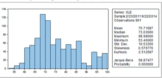
requires buying all of the securities represented in the energy index. Fund has a minimum of 95% limit for extreme cases for buying the assets in the exchange. This index include oil, gas and consumable fuels; and energy equipment and services. The companies selected are also in S and P 500 index. The variable is denoted as XLE (like in the NYSE) shortly in for this paper in the analysis. The Figure 1 below provides descriptive statistics for the variable XLE.

Teucrium WTI Crude Oil ETF provides access to crude oil investment through futures. The fund is unleveraged and diversified with instruments of different maturities. This reduces contango and backwardation and minimizes maturity risk. The daily changes in net asset value of weighted average closing price in WTI crude futures is reflected to ETF price. The benchmark index is WTI Crude oil futures contracts, which are traded in NYMEX. The variable is denoted as CRUD (like in the NYSE) shortly in for this paper in the analysis. The Figure 2 below provides descriptive statistics for the variable CRUD.

United States Brent Oil ETF uses short term oil futures which are traded on ice futures exchange as the benchmark. Therefore the daily changes in Brent crude oil affects the performance of ETF. The duration of the contracts does in no circumstances exceed 6 weeks. Depending on market conditions fund sometimes invest

in other crude oil investments that are more liquid. The variable is denoted as BNO (like in the NYSE) shortly in for this paper in the analysis. The Figure 3 below provides descriptive statistics for the variable BNO.

The variables are tested with ADF methodology to check whether they are stationary. The test is applied under 5% level of significance. The test statistic for the variable BNO is higher than critical value with absolute values. This shows that variable BNO is stationary in level (I(0)). This variable will be used in level so there is no test for differenced series. The test statistic for variable CRUD however doesn’t exceed critical value. Therefore the variable isn’t stationary in level. The variable is then tested with its first difference where test statistic is higher than critical value. This means that the variable CRUD is stationary with its first difference (I(1)). The test statistic for variable XLE fail to exceed critical value. Therefore the variable isn’t stationary in level. The variable is then tested with its first difference where test statistic is higher than critical value. This means that the variable XLE is stationary with its first difference (I(1)).

The variables are tested also with respected PP methodology to check whether they are stationary. The findings are the same. The test is applied under 5% level of significance. The test statistic for the variable BNO is higher than critical value with

Figure 1: Histogram and descriptive statistics for the variable XLE

absolute values. This shows that variable BNO is stationary in level (I(0)). This variable will be used in level so there is no test for differenced series. The test statistic for variable CRUD however doesn’t exceed critical value. Therefore the variable isn’t stationary in level. The variable is then tested with its first difference where test statistic is higher than critical value. This means that the variable CRUD is stationary with its first difference (I(1)). The test statistic for variable XLE fail to exceed critical value. Therefore the variable isn’t stationary in level. The variable is then tested with its first difference where test statistic is higher than critical value. This means that the variable XLE is stationary with its first difference (I(1)). These findings are presented in Table 1.

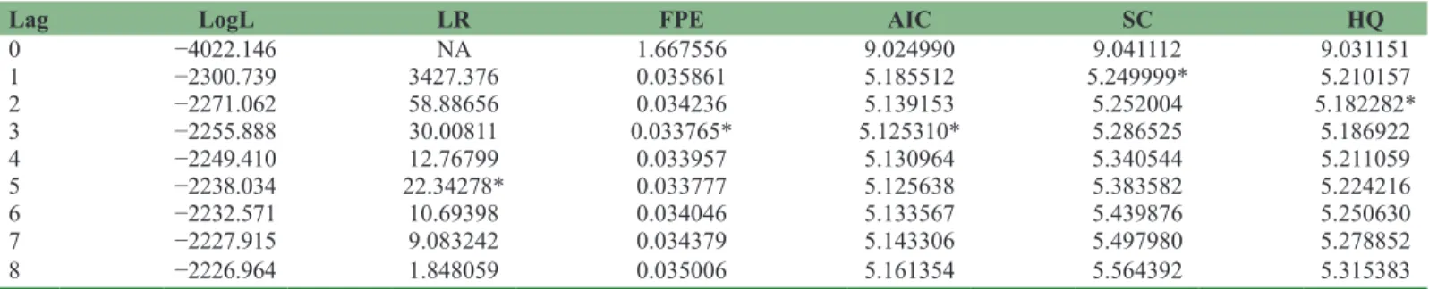
The variables BNO (in level), D(XLE) and D(CRUD) are tested to be with VAR. (VAR) First lag length is determined with selection criteria. According to Table 2, Schwarz information criterion 1 lag is suggested. Hannan-Quinn suggests 2 lags, Final prediction error and Akaike suggests 3 lags. For the principle of parsimony,

1 lag is used as suggested by Schwarz information criterion. 1 lag model - VAR(1) is developed for most degrees of freedom. VAR(1) model with inserted coefficients is given below. D(XLE)=−0.0236144462846*D(XLE(−1))+0.011845650094 *D (CRUD(−1))-0.0120636442044*BNO(−1)+0.511881384436 D(CRUD)=0.107683738179*D(XLE(−1))−0.149917215877*D (CRUD(−1))− 0.00554718257705*BNO(−1)+0.210270842466 BNO=0.0116398272568*D(XLE(−1))−0.0499537852161*D(CR UD(−1))+0.979721715954*BNO(−1)+0.822174262873

The model is checked for robustness. This is done by checking AR roots. For any autoregression model all the roots should be within the unit circle. This is to say the modulus should be less than one for the model to be reliable. According to Table 3, no roots are outside the unit circle, so the model passes the stability check.

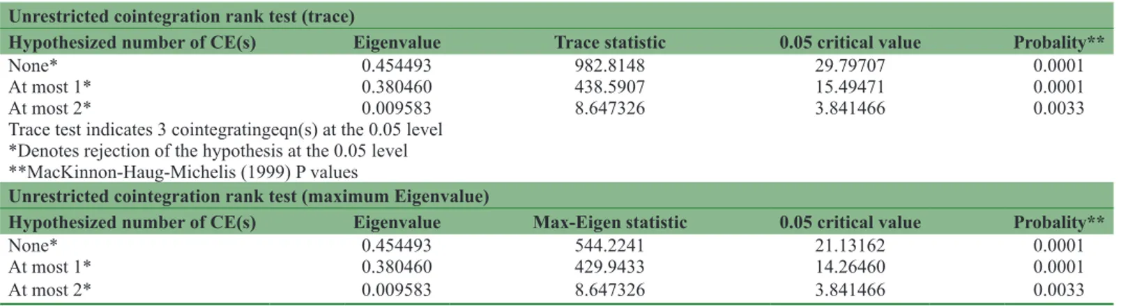
Cointegration test is made to check the long-run relationship between the variables. The test is made according to Trace and max eigenvalue methodology. According to both tests there are 3 cointegrating equations among the variables. This means the variable D(XLE), CRUD, and BNO is cointegrated. This is an important result since we have I(1) data in our model. The results are presented in Table 4.

Figure 3: Histogram and descriptive statistics for the variable BNO

Table 2: Lag length selection criteria for VAR model

Lag LogL LR FPE AIC SC HQ

0 −4022.146 NA 1.667556 9.024990 9.041112 9.031151 1 −2300.739 3427.376 0.035861 5.185512 5.249999* 5.210157 2 −2271.062 58.88656 0.034236 5.139153 5.252004 5.182282* 3 −2255.888 30.00811 0.033765* 5.125310* 5.286525 5.186922 4 −2249.410 12.76799 0.033957 5.130964 5.340544 5.211059 5 −2238.034 22.34278* 0.033777 5.125638 5.383582 5.224216 6 −2232.571 10.69398 0.034046 5.133567 5.439876 5.250630 7 −2227.915 9.083242 0.034379 5.143306 5.497980 5.278852 8 −2226.964 1.848059 0.035006 5.161354 5.564392 5.315383

*Indicates lag order selected by the criterion. LR: Sequential modified LR test statistic (each test at 5% level), FPE: Final prediction error, AIC: Akaike information criterion, SC: Schwarz information criterion, HQ: Hannan-Quinn information criterion, VAR: Vector autoregression

Table 1: Augmented Dickey-Fuller and PP test results

Model ADF test

crıtıcal value statıstıcTest crıtıcal valuePP test statıstıcTest

BNO −2.8645 −3.1101 −2.8645 −3.0093 CRUD −2.8645 −2.7147 −2.8645 −2.6338 XLE −3.4115 −2.9845 −1.9412 0.6668 D(CRUD) −1.9412 −32.22 −1.9412 −32.19 D(XLE) −1.9412 −30.61 −1.9412 −30.70

To test the short run relationship among the variables VECM(1) - VECM with one lag is developed. Differenced series for XLE and CRUD, and BNO in level is used for regression. The model with substituted coefficients is given below.

D ( X L E , 2 ) = 0 . 0 1 3 3 9 0 3 7 0 5 4 2 3 * ( D ( X L E ( − 1 ) ) -4.40493387505*D(CRUD(−1))+0.0152631002818* BNO(−1)-0.684215817684)−0.462598756341*D(XLE(−1),2 )+0.0628008941327*D(CRUD(−1),2)-0.553787639821*D(B NO(−1))−0.000810155617473 D ( C R U D , 2 ) = 0 . 2 9 3 7 6 9 7 6 8 6 5 5 * ( D ( X L E ( − 1 ) ) − 4 . 4 0 4 9 3 3 8 7 5 0 5 * D ( C R U D ( − 1 ) ) + 0 . 0 1 5 2 6 3 1 0 0 2 8 18*BNO(−1)-0.684215817684)−0.14750935372*D(XLE(−1), 2)+0.0580699809554*D(CRUD(−1),2)+0.108753698777*D(B NO(−1))−0.00198005307708 D ( B N O ) = 0 . 0 0 7 3 9 4 2 9 1 8 6 6 5 6 * ( D ( X L E ( − 1 ) ) - 4.40493387505*D(CRUD(−1))+0.0152631002818*BNO(−1)-0.684215817684)−0.00501435687067*D(XLE(−1),2)+0.0 0793526657202*D(CRUD(−1),2)−0.0679807866109*D(B NO(−1))+0.00169334201357

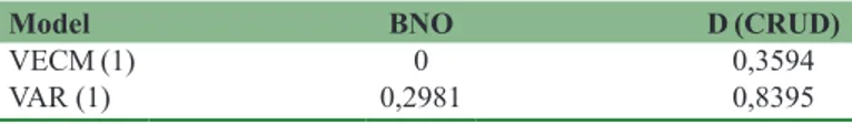
Finally the variables are tested for Granger Causality. The test is run both with VAR(1) and VECM (1) to test for long run and short run effects respectively. The test is applied to check whether BNO or D(CRUD) Granger causes D(XLE). According to Table 5, in the short run (with VECM(1))BNO Granger causes XLE, no other Granger causality is detected for 5% level of significance.

5. DISCUSSION

The variables representing Brent crude oil, WTI crude oil, and Energy Industry are checked to see whether they are stationary. This is done according to ADF and PP methodology. Both test indicate that Brent crude oil is stationary in level, whereas WTI crude oil and XLE.

The variables are modeled with VAR and VECM. This is done by first testing number of lags in the model where 1 lag is chosen as suggested by Schwarz Information Criterion. The VECM(1) is run for the short run and VAR(1) for the long run analysis. AR roots table also support stability of the models since all the roots are within the circle. The cointegration results according to Johansen procedure also indicate that the variables are cointegrated. The final test is Granger causality. This is to see which index which index provide better explanation in the energy industry. According to Granger causality results, Brent oil explains Energy industry perfectly in the short run. This is to say, Brent crude oil index is a better indicator of explaining energy industry in the short run. However in the long run this effect disappears. WTI doesn’t have a statistical explanatory value for energy industry.

6. CONCLUSION

According to the research, Brent crude is statistically an excellent indicator of energy industry in the short run. Brent traditionally is a better global benchmark although once taken over by WTI. This means Brent crude is now more reliable in representing oil industry. WTI, being an American index from Texas region, fails to represent energy industry for the research period statistically. This is an early warning signal for USA, and there is a lot to do for marketing and balancing the supply for WTI, which despite its superior quality loses market penetration.

Another finding of the study is that there is no relationship between oil and energy industry in the long run. This is partly because long extraction and refinement period for crude oil. This result

Table 4: Cointegration results

Unrestricted cointegration rank test (trace)

Hypothesized number of CE(s) Eigenvalue Trace statistic 0.05 critical value Probality**

None* 0.454493 982.8148 29.79707 0.0001

At most 1* 0.380460 438.5907 15.49471 0.0001

At most 2* 0.009583 8.647326 3.841466 0.0033

Trace test indicates 3 cointegratingeqn(s) at the 0.05 level *Denotes rejection of the hypothesis at the 0.05 level **MacKinnon-Haug-Michelis (1999) P values

Unrestricted cointegration rank test (maximum Eigenvalue)

Hypothesized number of CE(s) Eigenvalue Max-Eigen statistic 0.05 critical value Probality**

None* 0.454493 544.2241 21.13162 0.0001

At most 1* 0.380460 429.9433 14.26460 0.0001

At most 2* 0.009583 8.647326 3.841466 0.0033

Max-eigenvalue test indicates 3 cointegrating Eqn(s) at the 0.05 level. *Denotes rejection of the hypothesis at the 0.05 level. **MacKinnon-Haug-Michelis (1999) P values

Table 3: AR roots table

Root Modulus

0.979884 0.979884

−0.159148 0.159148

−0.014546 0.014546

No root lies outside the unit circle VAR satisfies the stability condition

has important implications for oil industry. The industry should actively look for alternative ways to extract and refine oil in less time consuming and more efficient ways.

Finally, as it is stated in this paper for WTI, one source of oil may not be adequate for explaining oil pricing. This has important consequences for traders and decision makers who rely on oil prices. In order to better grasp changes in the industry, there should be more sophisticating work on indexing oil. This will probably come with introducing a basket including oil such as Brent, WTI and perhaps Dubai. This is left for future studies in this field.

REFERENCES

Arnold, A., Liu, Y., Abe, N. (2007), Temporal causal modeling with graphical granger methods. KDD’07. p3.

Arouri, M.E.H. (2011), Does crude oil move stock markets in Europe? A sector investigation. Economic Modelling, 28, 1716-1725. Basher, S.A., Haug, A.A., Sadorsky, P. (2011), Oil prices, exchange rates,

and emerging stock markets. Energy Economics, 34, 227-240. Buyuksahin, B., Lee, T.K., Moser, J.T., Robe, M.A. (2013), Physical

markets, paper markets and the WTI-Brent spread. The Energy Journal, 34, 129-150.

Creti, A., Ftiti, Z., Guesmi, K. (2014), Oil price and financial markets: Mu ltivariate dynamic frequency analysis. Energy Policy, 73, 245-258. Gamarra, K.H., Sabogal, J.S., Faloon, E.C. (2015), A test of the market

efficiency of the integrated Latin American market (MILA) index in relation to changes in the price of oil. International Journal of Energy Economics and Policy, 5(2), 534-539.

Hatemi, J.A. (2012), Asymmetric causality tests with an application,

Empirical Economics, 43(1), 447-456.

Huang, W., Chao, M. (2012), The effects of oil prices on the price indices in Taiwan: International or domestic oil prices matter?, Energy Policy, 45, 730-738.

Hyalmarsson, E., Osterholm, E. (2007), Testing for Cointegration Using the Johansen Methodology when Variablesare Near-Integrated. IMF Working Paper. p5.

Kasibhatla, K.M. (2011), Does the dollar call the tune for securities and oil? An empirical investigation. The International Journal of Finance, 23(3), 6870-6880.

Lee, B., Yang, C.W., Huang, B. (2012), Oil price movements and stock markets revisited: A case of sector stock price indexes in the G-7 countries. Energy Economics, 34, 1284-1300.

Lee, Y.H. (2014), Dynamic correlations and volatility spillovers between crude oil and stock index returns: The implications for optimal portfolio construction. International Journal of Energy Economics and Policy, 4(3), 327-336.

Liao, H., Lin, S., Huang, H. (2014), Are crude oil markets globalized or regionalized? Evidence from WTI and Brent. Applied Economics Letters, 21(4), 235-241.

Priestley, M.B., Tong, H. (1973), On the analysis of bivariate non-stationary processes. Journal of Royal Statistic Society: Series B, 35, 135-166.

Schwert, G.W. (1989), Tests for Unit Roots: A Monte Carlo investigation, Journal of Business and Economic Statistics, 7(2), 156-158. Tao, S., Tang, D., Li, J., Xu, H., Li, S., Chen, X. (2010), Indexes in

evaluating the grade of Bogda Mountain oil shale in China. Oil Shale, 27(2), 180-188.

Virmani, V. (2001), Unit root tests: Results from some recent tests applied to select Indian macroeconomic variables. Indian Institute of Management, 3-5. Available from: http://www.iimahd.ernet.in/ publications/data/2004-02-04vineet.pdf.

Wang, Y., Wu, C., Yang, L. (2013), Oil price shocks and stock market activities: Evidence from oil-importing and oil-exporting countries. Journal of Comparative Economics, 41, 1220-1239.

Wei, C.C., Chen, C.H. (2014), Does WTI Oil price returns volatility spillover to the exchange rate and stock index in the U.S.? International Journal of Energy Economics and Policy, 4(2), 189-197.

Table 5: Granger causality probability table for D(XLE)

Model BNO D (CRUD)

VECM (1) 0 0,3594

VAR (1) 0,2981 0,8395