Q f i 1 -Ь ^ Ѳ
CONTINUOUS PROCESSING OF IMAGES
THROUGH
USER SKETCHED FUNCTIONAL BLOCKS
A THESIS
SUBMITTED TO THE DEPARTMENT OF COMPUTER ENGINEERING AND
INFORMATION SCIENCES
AND THE INSTITUTE OF ENGINEERING AND SCIENCES OF BILKENT UNIVERSITY
IN PARTIAL FULFILLMENT OF THE REQUIREMENTS FOR THE DEGREE OF
MASTER OF SCIENCE
By
Aydın KAYA
4 s ( A
I certify that I have read this thesis and that in my opinion it is fully adequate, in scope and in quality, as a thesis for the degree of Master of Science.
Assoc. Prof. Dr. Bülent ÖZGÜÇ (Principal Advisor)
I certify that I have read this thesis and that in my opinion it is fully adequate, in scope and in quality, as a thesis for the degree of Master of Science.
Prof. Dr. Mehmet BcCfay
I certify that I have read this thesis and that in my opinion it is fully adequate, in scope and in quality, as a thesis for the degree of Master of Science.
Assoc. Erof. Dr. Neşe Yalabık
Approved for the Institute of Engineering and Sciences:
Prof. Dr. Mehmet Baray, Director of Institute of Engineering and Sciences
ABSTRACT
C O N T IN U O U S P R O C E S S IN G O F IM A G E S T H R O U G H
U S E R S K E T C H E D F U N C T IO N A L B L O C K S
Aydın K A Y A
M .S . in Computer Engineering and Information Sciences
Supervisor: Assoc. Prof. Dr. Bülent Ö Z G Ü Ç June 1988
An object oriented user interface is developed for interacting with and processing images. The software prepared for this purpose includes image processing functions as well as user friendly interaction tools both of a lower level such as menus, panels, windows and a higher level such as a schematics. The lower level utilities provide direct interface with the available image processing functions. At the higher level, the nodes of the schematics serve as image processing function instantiations and the arcs are the paths through which processed images flow. By constructing such a schematics, a complex set of operations can be applied to images continuously.
Keywords : Image-processing, user interface design, window maneger, object-oriented programming.
ÖZET
K U L L A N IC IN IN Ç İZ D İĞ İ B L O K L A R L A S Ü R E K L İ
O L A R A K G Ö R Ü N T Ü İŞ L E M E
Aydın K A Y A
Bilgisayar Mühendisliği ve Enformatik Bilimleri Yüksek Lisans Tez Yöneticisi: Doç. Dr. Bülent Ö Z G Ü Ç
Haziran 1988
Görüntülerin işlemesi amacı ile nesneye yönelik bir bilgisayar, kullanıcı etkileşim sistemi geliştirilmektedir. Bu amaçla hazırlanan yazılım alçak düzeyde ve yüksek düzeyde kullanılabilen görüntü işleme foksiyonlarmı ve dostça kul lanıcı bilgisayar etkileşim elemanlarını içermektedir (pencereler, kontrol panoları , vs). Alçak düzeyde görüntü işleme fonksiyonları ile direk etkileşimli olarak çalışmak mümkündür. Yüksek düzeyde ise belli bir şekilde oluşturulan bir diagramm düğümleri görüntü işleme fonksiyonları yerine ve düğümler arasındaki bağlar ise işlenen görüntülerin takip edeceği yolların yerine geçmektedir. Böyle bir diagram aracılığı ile karışık bir operasyonlar kümesi sürekli bir şekilde uygulanabilmektedir.
Anahtar Kelimeler: Görüntü işleme, nesneye-yönelik programlama, çok pencereli iş düzeni, etkileşim sistemleri.
ACKNOWLEDGEMENT
I would like to thank my thesis advisor, Assoc. Prof. Bülent ÖZGÜÇ for his guidance and support during the development of this study.
I also appreciate my colleagues, Mesut Göktepe, Murat Karaorman, Ozan Azbazdar and Ahmet Coşar for their valuable discussions and comments.
I also thank my wife Beyhan Kaya for her understanding and patience during the development of this thesis.
TABLE OF CONTENTS
1 INTRODUCTION
1
2 OVERVIEW OF DIGITAL IMAGE PROCESSING
3
2.1 What is Digital Image Processing... 3
2.2 The Environment of Digital Image Processing 3 2.3 Basic Terminology of Raster Scan Display S y stem s... 5
3 IMAGE PROCESSING ALGORITHMS
7
3.1 Classification of the A lgorithm s... 73.2 Point P rocesses... 7
3.2.1 Contrast and Intensity Enhancement... 7
3.2.2 Histogram... 9 3.2.3 T h resh old... 11 3.2.4 D ith e r ... 11 3.3 Area P r o c e s s e s ... 13 3.3.1 Convolution... 14 3.3.2 M e d i a n ... 16 3.4 Geometric p r o c e s s e s ... 18 vi
3.4.1 R otation... 18
3.4.2 A v e ra g e ... 23
3.5 Frame Processes ... 26
4 IMPLEMENTATION OF THE SYSTEM
30
4.1 User Interface Design... 304.2 Object Oriented User In te rfa ce ... 31
4.3 Data Structures... 33
4.4 Direct M o d e ... 36
4.4.1 Available Functions ... 39
4.4.2 Colormap M anipulation... 41
4.5 Indirect M o d e ... 42
4.5.1 Representation of the Functions... 43
4.5.2 Operations on the B l o c k s ... 44
4.5.3 Constructing a Schematics... 45
4.5.4 Internal Representation of a Sch em atics... 46
4.5.5 Changing the Settings of Blocks in a Schematics . . . 49
4.5.6 Executing a S ch em a tics... 54
4.5.7 Modifying the Constructed Schematics... 56
5 CONCLUSION
57
REFERENCES
59
APPENDICES
A .l Introduction... 60
A .2 How to Start ? 60 A.3 Using the System in the Direct M o d e ... 61
A .4 An Example of Using the Direct M o d e ... 67
A .5 Changing the C o lo r m a p ... 70
A .6 Using the System in the Indirect M o d e ... 72
A .6.1 Introduction ... 72
A .6.2 Icons Representing the P roced u res... 73
A .6.3 The Operations On the B l o c k s ... 74
A .6.4 Constructing a Schematics... 76
A .6.5 Executing a S ch em a tics... 80
A .6.6 An Example of Using the Indirect M o d e ... 80
B ATTRIBUTE VALUES OF THE OBJECT INSTANCES
82
C T H E D A TA ST R U C T U R E S 88
LIST OF FIGURES
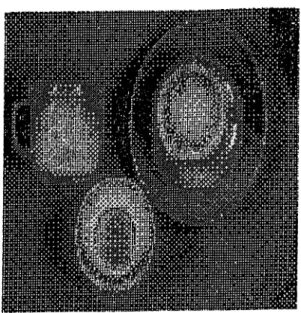
3.1 The "ORANGE” 8
3.2 Mirror image of t h e ’’ ORANGE” ... 8
3.3 The ” CUP” 9 3.4 The histogram of t h e ’’ ORANGE” 10 3.5 C code for the histogram algorithm... 10
3.6 The threshold of the ’’ ORANGE” with a threshold value 60 11 3.7 C partial code of the threshold a lg o r ith m ... 12
3.8 The dithered picture of the ” CUP” 14 3.9 C partial code for the dither algorithm ... 15
3.10 Horizontal lines of the ” CUP” have been a m p lifie d ... 16
3.11 Vertical lines of the ” CUP” have been amplified... 17
3.12 All lines of the ” CUP” have been a m p lifie d ... 17
3.13 All lines of the ” CUP” have been amplified and added to the original image 18 3.14 C partial code for the convolution algorithm ... 19
3.15 The dithered picture of the ” CUP” will be filtered by median filter with a 3 by 3 w in d o w ... 20
3.16 The result of the median filter 20 3.17 C partial code of the median f i l t e r ... 21
3.18 C partial code for the quick sort algorithm... 22
3.19 Rotation by 90 degrees 23
3.20 C partial code for the average algorith m ... 24 3.21 The "ORAN GE” has been s h r u n k ... 25 3.22 The "ORANGE” has been enlarged 25 3.23 The "ORAN GE” has been enlarged (another v ie w )... 26 3.24 The "ORANGE” AND its mirror i m a g e ... 27
3.25 OR of the images 27
3.26 XO R of the images 28
3.27 Addition of the images 28
3.28 Difference of the im a g e s ... 29
4.1 Data structure of the object list... 34 4.2 Data structures for average, histogram, convolution, and dither
b l o c k s ... 35 4.3 Data structures for threshold, median, AN D /O R, and point
operations blocks... 37 4.4 Data structures of the display, PLUS/MINUS, load, and save
functional blocks... 38 4.5 Layout of panel items ... 39 4.6 The colormap manipulation subwindow... 41 4.7 The menu associated with the CHOOSE PAINT STYLE key. 42 4.8 Operations on the blocks... 45 4.9 Data structure of the functional o b j e c t s ... 46 4.10 A schematics to find the AND of two images 47 4.11 The first object instance. 48
4.12 The final view of the object list. 48
4.13 The control window of the average b lo c k ... 49
4.14 The first control window of the convolution b lo c k ... 50
4.15 The second control window of the convolution b l o c k ... 50
4.16 The control window of the threshold b lo c k ... 51
4.17 The control window of the median b l o c k ... 52
4.18 The control window of the AN D /O R block ... 52
4.19 The control window of the point operations b lo c k ... 53
4.20 The control window of the load b lo ck ... 53
4.21 The control window of the save b lo ck ... 54
A .l Main window of the system... 61
A.2 The menu of the SAVE button... 62
A.3 The menu of the LOAD button... 63
A.4 The menu of the AVERAGE button... 64
A.5 The first window of the Convolution... 65
A.6 The second window of the Convolution... 66
A .7 The third window of the Convolution... 66
A .8 The result of dither operation. 68 A .9 The result of the threshold operation... 69
A. 10 The result of enlarging average... 69
A. 11 The result of shrinking average... 70
A. 12 The colormap manipulation window... 71
A. 15 The operations in the indirect m o d e ... 74
A. 16 Main frame and the schematics f r a m e ... 77
A. 17 An example of using the system in the indirect mode... 81
B . l The first object instance. 83 B.2 The first load instance... 83
B.3 The instance values after placing the second l o a d ... 84
B.4 The final attribute values of the object instance 1 ... 85
B.5 The final attribute values of the object instance 2 ... 85
B.6 The final attribute values of the object instance 3 ... 86
B. 7 The final attribute values of the object instance 4 ... 87
C . l The data structure of the functional object ... 88
C.2 The data structure of the average block... 89
C.3 The data structure of the histogram block... 89
C.4 The data structure of the convolution block... 89
C.5 The data structure of the dither block... 90
C.6 The data structure of the threshold b l o c k ... 90
C.7 The data structure of the median block 90 C.8 The data structure of the A N D /O R b l o c k ... 91
C.9 The data structure of the point operations b l o c k ... 91
C.IO The data structure of the display b lo ck ... 91
C .ll The data structure of the plus minus block ... 92
C.12 The data structure of the load b l o c k ... 92
A. 14 The icons representing the procedures... 73
1. INTRODUCTION
Digital image processing is the science of manipulating the digital representa tions of objects through a digital computer. Even if the history of this science is quite short compared to other fields, it has been used in many areas some of which are electronics, photography,and medicine.
Some people claim that transportation and data communication is in a very big competition and the winner will make the other one almost useless. If we accept this view, image processing becomes very important for the communication of people and information since it is an accepted fact that pictures or symbols convey messages better than other means. Supporting the above hypothesis there are currently many efforts to combine text and voice with images. Furthermore in a large number of software implementations, designers use symbols, icons, and images to provide a better and improved user interaction.
As there axe theorems, rules, procedures etc. in other sciences so are there for image processing. The procedures or algorithms of this science are mostly suitable to be implemented by a computer. In fact there are some image processors in the market and they implement some algorithms directly in the hardware. There are also some available image processing systems in which algorithms are implemented by programs, that is in the software. In most of the systems above the algorithms are usually implemented in such a way that the sequence of applying some algorithms to some images cannot be programmed at the beginning, but instead the user has to wait for the result of one procedure so that it can be used by another procedure. This strategy is clearly distracting in some applications like creation of instances of computer animation where the instances are slightly different from each other so that they can be obtained from the previous ones by making small modifications. This strategy can be used in systems where many different images are passed through the same process or an image is passed through
many image processing procedures and obtained images are stored for ani mation. If the user has enough skill he or she can arrange the processing procedures in such a sequence that many different instances of images can be obtained and saved without waiting for the intermediate results.
The image processing system described here allows two different modes for using the available image processing functions. The first mode of using the system is the direct mode in which image processing functions are invoked by just pressing some buttons in a control panel. On the other hand if the system is used in the second mode, namely in the indirect mode then a flowchart like diagram should be constructed. The constructed diagram which we call a schematics is used to select the image processing functions, their execution order and their inter dependency.
The organization of the following parts of this thesis is as follows. In chapter 2 an overview of digital image processing is given. This chapter also contains information about the environment of image processing and basic terminology of raster scan display systems.
Chapter 3 classifies image "processing algorithms and then describes the available image processing functions by giving examples.
Chapter 4 describes the implementation of the system in detail. In this chapter first the importance of the user interface is discussed and then using the system in the direct and indirect modes are explained by emphasizing the user interface. Internal representation of a constructed schematics and the execution strategy of a schematics are also explained.
Appendix A presents a user’s manual for those interested in using the system.
Appendix B gives instance values of nodes in a particular schematics. Finally appendix C presents the data structures in the C language.
2. OVERVIEW OF DIGITAL IMAGE
PROCESSING
2.1
W hat is Digital Image Processing
An image is a representation of an object and digital image processing is the science of manipulation of those representations by using a computer. The history of image processing is relatively recent compared to other fields but it has been applied to practically every type of imagery with varying degree of success, some of which are electronics, photography, pattern recognition and medicine.
Several factors encourage the future of image processing further. A major factor is the declining cost of computer hardware and the increasing avail ability of digitizing equipment (e.g. a TV camera interfaced to a computer) [9]. As a result now it is easy to store an image in the digitized form. An other factor, promoting image processing, is the availability of better display devices and low-cost but large main memories.
2.2
The Environment of Digital Image Processing
The main tool of image processing is a digital computer, in addition an input device to capture and digitize an image and an output device to display the processed image are needed. Images in their natural form are pictorial, that is they cannot be processed by the computer directly unless they are trans formed into numerical or discrete data. Therefore an image should first be converted into numerical form. This conversion process is called digitization and it generates an image in the form of a collection of dots, called picture elements or pixels. In a color system the value of each pixel (usually between
o and 255) is an index to a special table, which is called the colormap look-up table. The entry of the colormap table, corresponding to a particular index contains three values and these values are infact the intensities of three ma jor colors, namely red,green, and blue. In a gray scale device, same idea of referencing a table could be used or the value of a pixel could be treated as an intensity. The combination of all pixels form a rectangular grid or a 2-dimensional array, therefore any pixel can be addressed by specifying its address in terms of a row number and column number. Until relatively re cently, image digitizing was so expensive that only a few computing centers had such a capability. Advances in technology, however, are making image digitizers less expensive and their use more spread. An important and highly versatile type of image digitizer is the so-called digitizing camera, which has a lens system and can digitize an image of any object. An example is a television camera interfaced to a computer.
After an image is represented in numerical form, now it is possible to process it. That is a series of operations can be applied to it to obtain different forms of the original image. The operations to be applied to an image are classified according to the value of output pixels. If an operation generates an output pixel whose value is obtained by using only its previous value, this is called a point operation. A local operation is the one in which the value of a pixel is changed according to its old value and the values of neighbor pixels; this operation is sometimes called an area process. A global operation is the one in which all pixels of the image are treated in the same way. When the positions or arrangement of the pixels are changed this operation is called a geometric process. An opération changing the value of a pixel by comparing two or more images is called a frame process [1, 5].
After an image is processed and a desired image obtained, it is now nec essary to display it. There are two basic types of display devices, permanent and volatile. Permanent displays produce a hard copy image on paper, film, or other permanent recording medium. Volatile displays produce a tempo rary image on a display screen and these are used commonly in interactive processing. The primary characteristics that determine the quality of a dig ital image display system are the size, photometric and spatial resolution, low-frequency response, and noise characteristics of the display. The size of a display system has two components. The first of these is the physical size and the second is the size of the largest digital image that the display can handle. Clearly these components should be sufficient enough for an image to be examined when it is displayed and for an image to be displayed in its complete form.
Photometric resolution means the accuracy with which the system pro duces correct brightness or density value in each pixel position. The capacity of the number of bits per pixel that the display can handle varies from one display to another, for example a display system that can handle 8-bit of data can be used to display 256 different intensity values [9].
For the explanation of the other characteristics, please refer to [9].
Today the display devices and the supporting hardware have advanced features as compared to the old type of display devices. Now it is possible to store any kind of an image obtained through a CCD (charged coupled device) like a camera in a special memory called frame buffer or frame store in a very short time. For an image to be represented without losing the spatial resolu tion it is necessary to have a display device that has a resolution proportional to the number of different intensities in a picture. Each pixel can be repre sented by a definite number of bits, usually 1 byte, to represent a definite number of light intensities or color indices. In image processing systems the display devices are usually raster scan display systems so maybe to give a short information about these devices and the terminology associated with them is necessary.
2.3
Basic Terminology of Raster Scan Display Systems
The operation of raster scan systems to draw an image on the screen is different from other systems like random scan systems. The main difference of these systems is that, the storage is used to keep the intensity information for each screen position instead of storing graphics commands in random scan systems. For raster scan systems the refresh storage is usually called a frame buffer or a refresh buffer. Each position in the frame buffer is called a picture element or pixel. Pictures on the screen are painted from frame buffer one line at a time from top to bottom. Each horizontal line is called a scan line.
Pixel positions in the frame buffer are organized as a two- dimensional array of intensity values or references, which correspond to coordinate screen positions. The number of pixel positions in the frame or display buffer is called the resolution of the frame buffer. For an acceptable image to be displayed on the screen the resolution should be about 1024 by 1024, as suggested earlier.
In a simple black and white graphics and image processing system each
screen point is either on or off, that is we need to store only 1-bit of informa tion for each screen position or pixel in the frame buffer. For the more en hanced gray scale systems up to 24-bit information can be stored to represent many different intensities [1]. In colored display devices many combinations of three main colors (red,green and blue) can be displayed.
3. IMAGE PROCESSING ALGORITHMS
3.1
Classification of the Algorithms
Image processing algorithms can be classified in many ways. Here the clas sification criteria is the way of changing the pixels of a given image. As mentioned in section 2.2, if an algorithm changes a pixel’s value depending only on its value, it is called a point process. If the algorithm changes a pixel’s value based on its value and the values of the neighboring pixels it is called an
area process. If the algorithm changes the position or the arrangement of the
pixels it is called a geom etric process. Algorithms that change pixel values based on comparing two or more images are called fram e processes because a stored image is also called a frame [5].
In the following sections some image processing algorithms in the above classes are described and the results of applying them to three images given in figure 3.1, 3.2, and 3.3 are shown.
3.2
Point Processes
The available point processes or operations in the system axe, contrast and intensity enhancement, histogram, threshold, and dither, each of which is described and related resulting images are given below.
3.2.1
Contrast and Intensity Enhancement
This operation is useful for contrast and intensity adjustment which makes the original image sharper. To increase the intensity of some pixels their old
Figure 3.1: The ’’ ORANGE”
Figure 3.3: The ” CUP” values are increased by a constant value as in 1.
n ew .v alu e(x ) = old.valu e(x) + con stan t ( 1 )
As it is clear in this equation the selected pixels will be brighter or darker depending on the value of the constant added. To change the contrast of an image the only necessary thing to do is to multiply the values of the selected pixels by a constant. If we want both contrast and intensity adjustment at the same time we can use the formula 2.
n ew -valu e(x) = con stan ti * old-value(^x) + con stan t2 ( 2 )
3.2.2
Histogram
The histogram is a method of measuring an image. It is a different point process due to the fact that it does not change the value of the pixels.
The information provided by this operation is useful for image enhance ment. The histogram of the picture given in figure 3.4 for example can be used to detect the distribution of the pixel values in the image. The C code of the histogram algorithm is shown in figure 3.5. The function it performs is to count the number of times each intensity level occurs. The intensity level changes from 0 to 255.
Figure 3.4: The histogram of the ’’ ORANGE”
/ * Q partial code for histogram algorithm * /
int i, j, width, height, value; if (! pr_input) -C
printf("\n empty pixrect"); r e turn;
}
for (i=0; i < 255; i++) { histogram.array [i]=0;
}
width=pr_ input->pr_ s i z e .X ; height=pr_input->pr_size.y ; for (i=0; i < height; i++) {
for (j=0; j < width; j++) {
value=(int)pr_get(pr_input, j, i ) ; histogram.array[value]++;
}
Figure 3.6: The threshold of the ’’ ORANGE” with a threshold value 60
3.2.3
Threshold
Threshold is a global operation since it scans the values of all pixels. The pixel values are either changed to the lowest intensity (black) or to the highest intensity (white) depending on the value of a given constant and the value of the pixel. The constant used to compare to the values of the pixels are known as the threshold value which can range from 0 to 255. When the value of a pixel is less than the threshold value it is changed to 0 otherwise it is changed to 255.
The result of applying this operation is shown in figure 3.6 and the algorithm is presented in figure 3.7.
The threshold value is usually chosen to be the mid value of the intensities. The algorithm aims at increasing the visual resolution but also causes the fine details to be lost due to the large relative errors in displayed intensity for each pixel(e.g. if threshold value is 128 then there is no difference between the values 0 and 127 since both values will be changed to 0 in the final display). A technique developed by Floyd and Steinberg [2] distributes the large relative error to surrounding pixels to improve the details.
3.2.4
Dither
Dithering algorithm is a technique to increase the visual resolution without reducing the spatial resolution. This technique is used to display an image
int i,j, width, height, value, result; if (! pr_input) {
printf("\n empty pixrect"); return;
}
width=pr_input->pr_size.x ; height=pr_input->pr_size.y ; for (i=0; i < height; i++) {
for (j=0; j < width; j++) { value=(int)pr_get(pr_input, j, i ) ; if(value > threshold_value) pr_put(pr_input, j, i, F0REGR0UND_C0L0R); @Xs 0 pr_put(pr_input, j, i, BACKGR0UND_C0L0R);
/* C partial code for the threshold algorithm */
on a bilevel device and attempts to introduce a random error into the image. This error is added to the image intensity of each pixel before comparing with the selected threshold value. Adding a completely random error does not yield an optimum result. However, an optimum additive error pattern that minimizes pattern texture effects exists. The smallest dither pattern or matrix is 2 by 2. An optimum 2 by 2 matrix is
= 0 2
3 1 (3)
Large dither matrices are obtained by using the relation
T>n = 4T^n/2 4Dn/2 + 2C/„/2
4T>„/2 + 317n/2 4L)„/2 + Un/2 (4) where n is the order of the dither matrix and it should be equal to integer powers of 2 starting from 2 and U is the matrix of sizes n /2 by n /2 whose elements are all equal to one.
The algorithm compares the value of a pixel say in position x, y with the value of the element in position i,j where
i = X m od n , j = y m od n (n is the order of the matrix)
and if the value of the pixel in position x,y is equal to p(x,y) and it is greater or equal to the value of D(i,j) then the output pixel’s value becomes 1 otherwise its value is zero. Figure 3.8 shows a picture obtained by using the dither algorithm, and the C partial code for the algorithm is given in figure 3.9.
3.3
Area Processes
An area process uses neighborhood information to change the values of pixels. They are typically used for spatial filtering (such as filtering out repeated elements) and changing an image’s structure. They can sharpen the the image’s appearance besides removing noise, blurring or smoothing the image.
The available area processes in the system are convolution and median, which are described in the following sections.
pssiaiisa
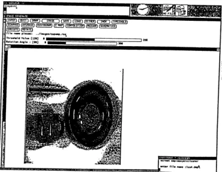
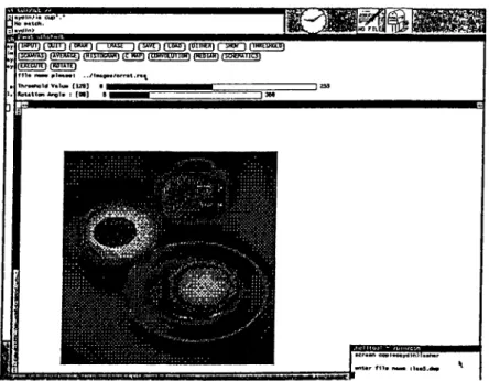
fW P D n ( T y r iT I í CiUWi f 'E l U a ~j f g V E I f n a i n (XITTHEffl r ~ 5 B 0 r n ( W a o C D l [SCAWA^'l |A\^ewac£ ] iH IS Io c h a h] (COWDLÜT11M) t S a W T I C S ) [tXEÜJitl (HOUTEl
f i l a riMM plaaaat . ,/lM g a a /cu p .r·^
Thraahotd Vilua (128] ■ — ---Hotitlon Angla i [M ]
Figure 3.8: The dithered picture of the ” CUP”
3.3.1
Convolution
Convolution is a classical image processing algorithm and it is used com monly for spatial filtering and finding the features of an image. The -basic convolution operation is the replacement of a pixel’s value with the sum of that pixel’s value and its neighbors by weighting each value by a factor. The weighting factors are called convolution kernel, every pixel value is replaced by the value p(x,y) where
p{x, y) = + m ,y + n) (5)
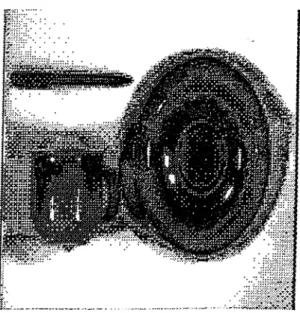
M and N are the sizes of the convolution kernel matrix. By using different kernels it is possible to amplify vertical, horizontal or all edges in an image [5]. Figures 3.10, 3.11 , and 3.12 show how this can be achieved.
The convolution kernels below are used to amplify the vertical, horizontal and all edges of an image respectively.
K v = - 1 0 1 \ - 1 0 1 - 1 0 1 - 1 0 1 ^ - 1 0 1
y
(
6)
/* C partial code for the dither algorithm */
■c
int i, j, k, 1, value, width, height, result; if (! pr_input) {
printf("\n empty pixrect"); retu r n ; > width=pr_ input->pr_s i z e .x ; he ight=pr_ input->pr_ s i z e .y ; colormapCO][FOREGROUND.COLOR] colormapCl][FOREGROUND.COLOR] colormap[ 2 ][FOREGROUND.COLOR] colormap[0][BACKGROUND.COLOR] colormapCl][BACKGROUND.COLOR] colormap[ 2 ][BACKGROUND.COLOR] (u.char)O; (u.char)O; (u.char)O; (u.char)255; (u_char)255; (u.char)255; for (i=0; i < height; i++) ■[
k=i ·/. 16; for (j=0; j < width; j++) { l=j 7. 16; value=(short)pr.get(curr.dither->pr_input, j, i) ; if (value >= d[k][l]) pr.put(curr.dither->pr_input, j, i, FOREGROUND.COLOR); else pr.put(curr_dither->pr.input, j, i, BACKGROUND.COLOR);
Figure 3.9: C partial code for the dither algorithm
Figure 3.10: Horizontal lines of the ” CUP” have been amplified 1 - 1 - 1 - 1 - 1 - 1
\
==
0 0 0 0 0 1 1 1 1 1 1/
1 - 1 - 1 - 1^
K a = - 1 8 - 1 1 - 1 - 1 - 1 J (7)(
8)
If we slightly modify the last kernel, by making the value in the center 9 instead of 8 the resultant image obtained is the same as if we added the original image to the image in figure 3.12 and the resulting image becomes sharper as shown in figure 3.13.
The partial code of this algorithm is given in figure 3.14.
3.3.2
Median
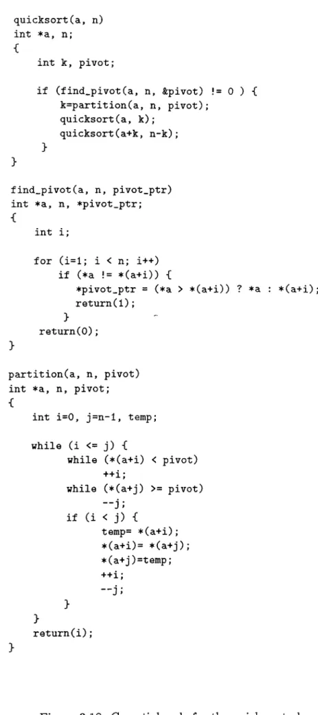
Median filtering replaces the pixel at the center of a neighborhood of pixels by the median of pixel values. The neighborhood pixel values are sorted in ascending order and the median(middle) value is used to replace the center pixel. This algorithm for which the code is in figure 3.17 and in figure 3.18,
Figure 3.11: Vertical lines of the ” CUP” have been amplified
Figure 3.12: All lines o f the ” CUP” have been amplified
Figure 3.13: All lines of the ” CUP” have been amplified and added to the original image
is used to remove the salt and pepper noise from an image ( Figures 3.15 and 3.16) [5].
3.4 Geometric processes
The algorithms or processes obtaining a new image by changing the pixel positions of an original image are called G eom etric Processes. Two such pro cesses available in the system are rotation by an arbitrary angle and average.
3.4.1
Rotation
This algorithm is used to rotate an image with respect to its center by an angle between 1 and 360 degrees. The result of rotating the image in figure 3.1 by 90 degrees is given in figure 3.19.
int i, j, k, 1, width, height, value, rel_x, rel_y, row, column, coll; Pixrect *pix;
if (! pr) return; width=pr->pr_size.x ; height=pr->pr_size.y ;
pix=mem_create(width, height, pr->pr_depth); rel_y=(int)(row_num/2.0);
rel_x=(int)(column_num/2.0);
for (i=rel_y; i < height-rel_y; i++) { for (j=rel_x; j < width-rel_x; j++) {
value=0; row= -1;
for (k=i-rel_y; k <= i+rel_y; k++) { row++; column= -1;
for (l=j-rel_x; 1 <= j+rel_x; 1++) { column++; value=(int)(value+convol_mat[row][column] * (int)pr_get(pr, 1, k)); } } if (value > FOREGROUND.COLOR) { value=F0REGR0UND_C0L0R; }
pr_put(pix, j,i, value);
} }
/* C partial code of the convolution */ int row.num, column.num, *convol_mat;
Figure 3.14: C partial code for the convolution algorithm
Figure 3.15: The dithered picture of the ” CUP” will be filtered by median filter with a 3 by 3 window
/* C partial code for the median filtering */ int row_num, column.num;
int i, j, k, 1, width, height, value, rel_x, rel_y, row, coliimn, el_num, value;
int *median_array, *temp; Pixrect *pix;
if (! pr) return; width=pr->pr_size.x; height=pr->pr_size.y ;
pix= mem_create(width, height, pr->pr_depth); median_array = (int *)
malloc(sizeof(int)*row_num*column_num); if (! median_array) {
printf("\n error in array median !"): r e t u r n ;
>
rel_y=(int) (row_nvmi/2.0) ; rel_x=(int)(column_num/2.0); for (i=0; i < height; i++) {
for (j=0; j < width; j++) { el_num=0;
temp=median_array;
for (k=i-rel_y; k <= i+rel_y; k++) { if (k >= 0 && k <= height) {
for (l=j-rel_x; 1 <= j+rel_x; 1++) { if (1 >= 0 M 1 <= width) { el_num++; *temp=(int)pr_get(pr, 1, k ) ; temp++; } } } } quicksort(median_array, el.num); value = (int)(*(median_array+(int)(el_num/2.0)))); pr_put(pix, j, i, value); > }
Figure 3.17: C partial code of the median filter
quicksort(a, n) int *a, n; ■C int k, pivot; if (find_pivot(a, n, &pivot) != 0 ) { k=partition(a, n, pivot); quicksort(a, k ) ; quicksort(a+k, n - k ) ; } find_pivot(a, n, pivot_ptr) int *a, n, *pivot_ptr;
int i;
for (i=l; i < n; i++) if (*a != *(a+i)) {
*pivot_ptr = (*a > *(a+i)) ? *a : *(a+i); return(l);
}
r e turn(0);
partition(a, n, pivot) int *a, n, pivot;
{
int i=0, j=n-l, temp; while (i <= j) {
while (*(a+i) < pivot) ++i;
while (*(a+j) >= pivot) if (i < j) { temp= *(a+i); *(a+i)= *(a+j); *(a+j)=temp; ++i; " j ; > } return(i);
fTBWT) f pun ) fPBJW ) f 3 ( 5AVT ) [ LDU ) (PITHEai [ show j [IHaCSHOCin
[5CAWAS1 [AVfciUcitl (H n iD W A H ) [ t kAP) faW TC nniB ITI (HEBUM) f S C H W T l O l (W U IE · )
r i ) · n · « · p l · · · · ı . . / ( M g n / e r r a t .n ^ ThrMhold ValiM [ 128] · ■ ■ ■ ■ ■ i RoUtlan Angla : [M ]
] #■
Figure 3.19: Rotation by 90 degrees
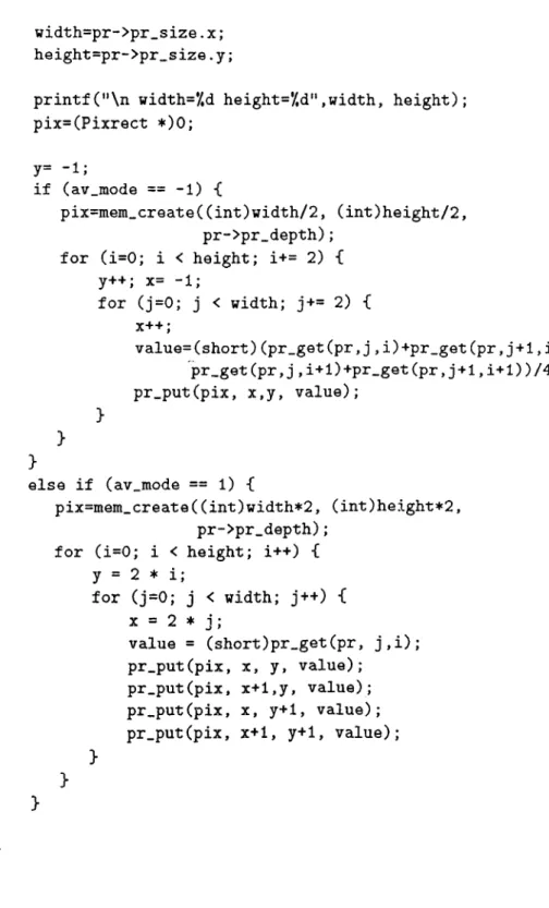
3.4.2
Average
Averaging is an algorithm that can be used for both enlarging and shrinking images. Shrinking average takes the pixels of an image in groups of four (2 horizontal and 2 vertical pixels) and produce an output pixel whose value is equal to the average of values of these four pixels (Figure 3.21).
Enlarging average takes a pixel and copies its value to its four neighbors. As a result the original image is enlarged by a factor of four (Figures 3.22, 3.23).
The algorithm in figure 3.20 can be used for both enlarging and shrinking a given image.
Average algorithm is used when a user wants the fine details of an image to disappear or when an image is wished to be displayed in the form of blocks besides changing the size of an image. This can be achieved by applying shrinking algorithm and then enlarging the image continuously.
/* C partial code of the average algorithm */ int i,j, X, y, value, width, height; Pixrect *pix;
width=pr->pr_size.x ; height=pr->pr_size.y;
printf("\n width='/,d height='/,d",width, height); pix=(Pixrect *)0;
y= -1 ;
if (av_mode == -1) {
pix=mem_create((int)width/2, (int)height/2, pr->pr_depth);
for (i=0; i < height; i+= 2) { y++; x= -1;
for (j=0; j < width; j+= 2) { X++;
value=(short)(pr_get(pr,j,i)+pr_get(pr,j +1,i) + pr_get(pr,j,i+1)+pr_get(pr,j+l,i+l))/4; pr_put(pix, x,y, value);
}
else if (av_mode == 1) {
pix=mem_create((int)width*2, (int)height*2, pr->pr_depth);
for (i=0; i < height; i++) { y = 2 * i;
for (j=0; j < width; j++) { X = 2 * j;
value = (short)pr.get(pr, j,i); pr_put(pix, X, y, value);
pr_put(pix, x+l,y, value); pr_put(pix, X, y+1. value); pr_put(pix, x+1, y+1, value);
( u M i i ) t Q Uil ) [ WaV 1 t EKA5E ] [ SAV£ ) [ LtUfl ] n n T K fin [ Si<№ j ( T t t f O f l L D j i5CA^^A3i u v E j a g · ) im siPC JUM ) tc xx**·] ( a w o L U T iP in (HEPuroi (s c h o u t i c s i
(TgnnEI
Figure 3.21: The "ORANGE” has been shrunk
rrotm ropin rcHBn r-rwsrn igEgm} ' fSOWASl fAVEmCT) fHISTD<WHl P T W ) icnwoLUiiuH) [HtoLAHj (SChWiU^S»)
fEyECinil [HOiAtE]
, ft I· i>MM pi····: ../1no*a/or««.ra^ 7hr*«iiald V ilu · (1 3 ·] · - RoUtlen Angl· : ( 06]
Figure 3.22: The "O R A N G E ” has been enlarged
Figure 3.23: The ’’ ORANGE” has been enlarged (another view)
3.5
Frame Processes
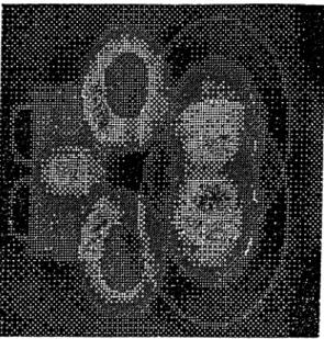
Frame processing algorithms are used to obtain a new image by using the pixel values of two or more images. Common algorithms in this class are diiFerence that can be used to find out missing parts between two images. Addition of images is used to enhance an image or to obtain an image whose pixel values are the average of the pixel values of the processed images. AND operation is used to mask some parts of an image by using a mask image and OR operation combines two or more images into one [5] ( Figures 3.24, 3.25, 3.26, 3.27, 3.28).
Figure 3.24: The ’’ ORANGE” AND its mirror image
Figure 3.25: O R o f the images
Figure 3.26: XO R of the images
Figure 3.28: Difference of the images
4. IMPLEMENTATION OF THE SYSTEM
4.1
User Interface Design
When the performance of the user interface of an application (i.e the part of the system that determines how the user and the computer communicate) cannot be predicted it is very likely that users will react in unexpected ways when they use the system for the first time.
It is very important to pay careful attention to the design of interactive user interfaces. Bad user interfaces are not only difficult to learn but they also make a system inefficient to operate even in the hands of an experienced user. In extreme cases an entire system may be invalidated by poor user interface design, that is, it may prove impossible to train users to operate the system, or the user interface may be so inefficient and unreliable that the cost of using the system cannot be justified [4, 6].
Since our aim is to implement an image processing system through the use of functional blocks, and a functional block means the representation of a routine or function by a visual object in our intent, writing a user interface in old fashion (in the form of command languages) cannot be justified. In the traditional user interfaces command languages were heavily used to provide communication between the user and the computer. In this kind of user interface the user has to know the exact syntax of the available commands. For example, when someone wishes an image to be saved on the disk he or she has to give a command like
save(image,file-name)
where image is a pointer to a particular section of memory where the storage of the the image begins or the name of an array storing the image, and file-name is a string denoting the name of the file to be saved.
Even in this simple example there are many complexities for a novice user. First he has to remember the exact syntax of the command,second he should know about some other commands like accessing the value of a pointer, opening and closing a file.
An alternative to the above method is to represent a save function by an icon and when it is selected through a pointing device like a mouse, display the listing of images that the user can save, and then ask a name under which the image will be saved. The use of such methods leads us to some new concepts in software sciences, most important of which are the object oriented style or discipline of programming, iconic interface and use of multiple windows. Although our intention in this thesis is not to talk about these concepts in detail it is better to explain the user interface that we plan to employ by considering the ideas behind these new and important software techniques.
4.2
Object Oriented User Interface
From the previous section it can be assumed that a user interface in the form of a command language cannot be justified in a work like ours. Therefore we planned a user interface that is very user friendly and based on a toolkit, namely on the Sun View^^ presenting menus, windows, panels, and many kinds of items(sliders, buttons, choices, etc.) ready for special usage as com ponents of the user interface. The components in a toolkit are usually used by a pointing device like a mouse as long as there is no need to enter text. These components have the characteristics of an object in the sense of object oriented programming style even if they may be implemented by using an ordinary language like C [10].
As previously stated the building blocks of the user interface are the vi sual representations of the various objects in the form of icons, data template windows, control panel items like buttons, sliders, choices etc. It is very important to note that the term object refers to both an entity in the real life,like a picture or a chair etc, and the term ’’ object” in the ’’ object ori ented style of programming” . The difference should be understood from the context.
The object classes of the functional blocks, the panel items and menu choices represent the available options to the user. The objects provided have their particular properties and the user tells the system what kind of
processing he wants by selecting a particular icon representing an object in a particular class and connecting those like a simple flowchart which we call a schem atics. By pointing to the instances of various object classes in the schematics by the aid of the mouse, the properties of that object instance could be changed as explained later.
One of the most important kind of object classes (groups of object instan tiations) used in our system are data template windows and they axe used to set the arguments of various object instances (object variables) and to display an intermediate image in the process if the functional block happens to be a display device. Other visual object classes except the window are the class of menus, class of scrollbars and the functional blocks represented in the form of icons.
Icons are small pictures (usually they are composed of 64 by 64 pixels) and they represent available functions to be applied to the images, menus are used to select a particular choice for an object, and scrollbars are used to view different parts of an image both in vertical and horizontal directions [3].
Technically speaking an object is an entity presenting a functional in terface. The implementation of how the objects perform their jobs are not exposed to the user, instead it is enough to choose a particular object and set the variables belonging to it. When an object is chosen it calls its asso ciated functions in an indirect manner, that is there is not a main program that calls a function or routine in a proper order, instead all objects are active processes(in a multi- programming environment) and their associated functions or routines are called through user or system invoked events. The associated routines of an object may also be called by another object. When an object is to be invoked it is necessary to form a proper message and send it.
The objects and object classes form a hierarchy. In this sense the object is at the most upper level, below it we have object classes, namely menus, windows,scroll bars, and functional blocks, displayed to the user in the form of icons. Each class may contain many instantiations of objects for example a window may contain panels, text sub windows, drawing windows, and a panel may be further subdivided into many panel items.
4.3
Data Structures
The data structures of the image processing algorithms together with their describtion are given in figures 4.1 through 4.4. In these figures the data structures are presented by diagrams. The corresponding C structures are given in appendix C.
Currently there are 12 functional blocks representing one or more func tions. Each of them is represented by a linked list that can be reached through the general linked list representing any object, namely the object list.
The linked list object list in figure 4.1 represents any kind of object. It contains information about the object it is representing(instance, and object id), position of particular object instance , and the links connected to a particular instance.
The diagrams in figure 4.2 represents the data structures for four of the 12 functional classes. These are average, histogram, convolution, and dither functional blocks. Each data structure for functional blocks contain common information for the instance number of the class, the colormap of an instance, a pointer to an image that is to be processed, and a pointer to the next instance in the same class.
Besides the common information kept in each functional block, there are some special attributes for almost all functional blocks in each class. The
opr field of the average block keeps information so that either enlarging or
shrinking average operation can be applied.
The histogram array of the histogram block is used to keep the count of pixels in each intensity between 0 and 255. The convolution block stores information related to the size of convolution kernel (row, and column num ber), and the entries of it. The dither block keeps information for storing the size and entries of the matrix to be used in the dither operation.
Figure 4.2 shows the diagrams of the data structures for threshold, me dian, A N D /O R , and point operations blocks. The private information be longing to these blocks are explained below.
The threshold value in the data structure of the threshold block stores the the threshold that is to be applied in the threshold operation. Median block
OBJECT LIST
INSTANCE NO. OBJECT ID. POSITION X POSITION Y NEXT PIN POSITION
NEXT PIN POSITIO NS PRE. PIN POSITION 1
PRE. PIN POSITION 5
NEXT OBJ 1
— ^ NEXT OBJ 5 PRE. OBJ 1
PRE OBJ 5 NEXT
Figure 4.1: Data structure of the object list.
AVERAGE BLOCK 255 INSTANCE OPR. MODE COLORMAP ENTRIES TO IMAGE NEXT HISTOGRAM BLOCK 255 255 INSTANCE ENTRIES COLORMAP TO IMAGE HISTOGRAM ARRAY NEXT 255 CONVOL BLOCK INSTANCE ROW NUMBER COL. NUMBER COLORMAP ENTRIES TO IMAGE HISTOGRAM ARRAY CONVOL ARRAY NEXT DITHER BLOCK 255 INSTANCE ROW NUMBER COL. NUMBER COLORMAP ENTRIES TO IMAGE HISTOGRAM ARRAY 0 6*16 DITHER ARRAY NEXT
Figure 4.2: Data structures for average, histogram, convolution, and dither blocks
keeps the size of median filtering window in terms of row and column num ber. A N D /O R block is used in the frame processing involving two images. Therefore it stores another pointer to an image and the operation code. This operation is one of AND, OR, XOR, PLUS, and MINUS operations. The pri vate data for the point operations block contains the intensity, contrast, and a function pointer. The first two attributes are used in image enhancement. The function pointer points to a point operation function to be used for this particular instance.
The data structures for display, PLUS/MINUS, load, and save blocks are in figure 4.4.
As it is shown in figure 4.4 the display block does not contain any special information. The PLUS/MINUS block is designed for frame processing oper ations. Therefore it contains one more pointer to an image and the code for type of frame processing. The load and save functional blocks both contain the name of a disk file that an image is to be loaded from or an image is to be stored into.
In the system there are two modes or styles of interaction. These are named as Direct mode and Indirect mode. In both of the modes the user can use every function that he or she likes.
4.4
Direct M ode
This mode of operation is especially useful when the user does not want to construct a schematics for some trivial operations, that is any kind of operation that can be performed without doing anything else before. Loading an image or saving an image from or to disk are clearly trivial or simple operations in this sense.
In this mode directly applicable or trivial operations are invoked by just pressing a suitable panel button by the mouse. The user also has to supply a file name for some operations, such as save or load an image. The result ing image is displayed immediately after the operation is completed and it becomes the current image to be used in later operations until a new image
THRESHOLD BLOCK 255 INSTANCE THRES. VALUE MEDIAN BLOCK COLORMAP 0 ENTRIES 255 TO IMAGE NEXT INSTANCE ROW NUMBER COL. NUMBER ENTRIES COLORMAP TO IMAGE NEXT AND/OR BLOCK 255 INSTANCE OPR. ID. COLORMAP ENTRIES TO IMAGE 1 TO IMAGE 2 NEXT
POINT OPERATIONS BLOCK INSTANCE 255 INTENSITY CONTRAST COLORMAP ENTRIES TO IMAGE TO FUNCTION NEXT
Figure 4.3: Data structures for threshold, median, A N D /O R , and point op erations blocks.
PLUS MINUS BLOCK DISPLAY BLOCK 255 INSTANCE COLORMAP ENTRIES 255 TO IMAGE NEXT INSTANCE OP. ID. ENTRIES COLORMAP TO IMAGE 1 TO IMAGE 2 NEXT LOAD BLOCK 255 INSTANCE FILE NAME COLORMAP ENTRIES SAVE BLOCK 255 TO IMAGE NEXT INSTANCE FILE NAME COLORMAP ENTRIES -> TO IMAGE NEXT
Figure 4.4: Data structures o f the display, PLUS/M INUS, load, and save functional blocks.
r n g p - ) n n iH EB ) f iaVM I pTiBE M m (^CaWa s] [ W b a c t ] [H i^ io m A H i [C tU<»i (CflW DUJIID m (H E C IO n fr o O U TTCSI /TVC nitr^ ffln il 1P\ ^ * '■ - * llXfecuT£i fHOTi'TEl
f n · ruM p i · · · · ; ../1 m o «s/o rw )o a l.r·^ Thraahold Valu· [ 12fl]
Rotltlon Angla ; (09]
Figure 4.5; Layout of panel items
is loaded. As a result of this an image already processed in some way can be processed further.
4.4.1
Available Functions
When the system is started a window is opened through which some of the functions can be invoked directly. These functions are invoked by pressing a mouse button on one of the buttons shown in the top part of the screen (see figure 4.5).
As it is seen in figure 4.5 the available functions are as follows^ :
• ERASE : It clears the canvas^.
• SAVE : This is used to save an image which is on the screen or in the memory (current image) to disk in the raster file format. In raster file format every image has a 32 byte header to store the information about the length, width, depth (number of bits per pixel) of an image. After the header the related colormap is stored and it occupies 768 bytes. Finally the pixel values are stored in the file.
^The detailed descriptions of the functions are presented in Appendix A. ^Canvas is a drawing subwindow.
• LOAD : This function is used to load an image from the disk which has been stored in raster file format previously. Here one point to be stated is that loading or saving an image with sizes 512 by 512 is about two seconds.
• DITHER; The image which was loaded before or the image in the mem ory will be dithered and it will be displayed on the screen. The obtained image becomes the current image and other processing functions can be applied to it.
• SHOW : This function is useful for displaying an image not in raster file format and to store it in the raster file format for compatibility. • THRESHOLD : This function applies the threshold operation to the
image and the resulting image becomes the current image.
• SCANVAS : This is a function to save the whole drawing window or the canvas in a format which is suitable for printing by using an ordinary printer.
• AVERAGE : If someone wishes to enlarge or shrink the current image this function can be selected.
• HISTOGRAM : When the processing of the function is completed the histogram of the image will be displayed on the screen.
• C MAP : This function is used to change the colormap of the displayed image and to paint some portions of it in a simple manner.
• CONVOLUTION : This function is used to covolve an image with a convolution kernel that is a two dimensional table.
• MEDIAN : This button is used to pass the current image through the median filter to make it blurred or to remove salt and pepper noise. • SCHEMATICS : When this key is pressed the user can draw a schemat
ics to process the images in the indirect mode.
The construction of the schematics is described in detail in appendix A.
• EXECUTE : This button is used to execute a previously constructed schematics in the schematics canvas. •
• ROTATE : In the direct mode ROTATE button is used to turn an image with respect to its center by a definite angle.
Figure 4.6: The colormap manipulation subwindow.
4.4.2
Colormap Manipulation
The window shown in figure 4.6 is opened as a result of pressing the C MAP button. It has four slider items and two buttons.
The ’’ colormap index” slider is used to set the index of the colormap entries between 0 to 255. The index can also be set by pressing the middle mouse button in the canvas to see the color intensities of a particular pixel and its particular location in the colormap table.
The other sliders are used to change the intensities of three main colors, namely red, green, and blue from black (0) to white (255). By arranging these sliders a pixel value may have one of the over 16,000,000 colors. The affect of changing the values of color sliders is observed in real time. That is when a change of the color sliders is made the corresponding color value in the entry set by the colormap index will be changed immediately. As a result of this operations all the pixels of the image showing this entry will have another color at the same time.
The two buttons are used to paint the image on the canvas and to cycle the colormap entries respectively. The first button has a menu associated with it and is shown in figure 4.7. The menu items are POINTS, INJECTION, and BLOCKS that are used to put points, to make injection onto the image
(5CAWA5) (Я У Е Ш С Ц (TTTSTIglUHl ( П Т О П fC D W D U n iO in (НСРШ 11 ('SCHOUIICSI Retatl 2 et 1299 colomap Indu [9] гш4 1 (239] ■ 1 ' j 299 bill· ; (2991 (CHOUSE· PAIHT STVipSTiTi--- n
Figure 4.7; The menu associated with the CHOOSE PAINT STYLE key. and to paint the image with blocks respectively. When the painting style is chosen from the menu the user can paint the image just by pressing the right mouse button and dragging it on the canvas. The color used in the painting process is the one in the colormap entry which is set by colormap index and of course one of the over 16,000,000 colors can be in that entry.
The CYCLE MAP button is used to cycle the colormap entries by a certain amount to obtain different views of the displayed image when the pixel values jump from one color to another. This technique is used in many art works, advertisement, and animation.
4.5
Indirect M ode
This mode of operation is used to process the images in continuous fashion and especially useful when the user wants to see the intermediate or final results of some predefined processing sequences.
This mode involves construction of a schematics on the schematics can vas that describes the processing steps and their execution order like in an algorithm or a flowchart.
4.5.1
Representation of the Functions
The 12 available functions in the indirect mode are represented as icons which are also the representations of the menu items. The menu containing these representative icons is associated with the CHOOSE BLOCKS button in the SCHEMATICS FRAME. Any menu associated with the panel buttons are always displayed by pressing the right mouse button on the related panel button.
The represented functions are as follows:
• AVERAGE : which is used to shrink or enlarge an image. • HISTOGRAM
• CONVOL :Block representing the convolution operation. • DITHER
• THRESHOLD • MEDIAN
• A N D /O R : This block represents the frame operations which are AND, OR, XOR, addition of two images, and difference of two images.
• POINT OP : This icon represent the intensity and contrast enhance ment and it is possible to include more point operations in it.
• DISPLAY : This icon represent the display device. When another block is connected to it the stored image in that block will be transfered to the display block and be ready for displaying it.
• LOAD : It is used to load an image from the disk which should be in raster file format. •
• SAVE : Any image obtained in one of the processing steps can be stored in the disk in the raster file format when this block is connected to the block which contains the desired image.
4.5.2
Operations on the Blocks
The functions that affect the placement, location, selection, or the settings of any block in the BLOCKS MENU are the items of the OPERATIONS MENU. These functions are shown in figure 4.8, and listed below^.
• SELECT BLOCK TO REMOVE (F I) : After selecting this operation clicking the left mouse button or pressing the function key FI when the cursor in on a block causes the block to be removed from the schematics. • PUT BLOCK ON CANVAS (F2) : This operation is used to put a
selected block on the drawing window or the canvas.
• SELECT FIRST BLOCK (F3) : This operation together with the next one is used to select two connected blocks to disconnect the link between them.
• SELECT SECOND BLOCK (F4) : The second connected block is se lected similarly to the first block.
• CONNECT BLOCKS (F5) : Any pair of the blocks on the canvas can be connected after selecting this operation.
• DISCONNECT BLOCKS (F6) : This is used to disconnect two blocks already connected.
• UNDO (F7) : This operation is to cancel the last operation applied. • CLEAR ALL (F8) : When this operation is selected the schematics
constructed so fax is destroyed and the canvas is cleared.
• RESET EXECUTION FLAGS (F9) : As it is explained in ’’ Executing the Schematics” the execution of a schematics for a second time or later needs the execution flags of all the blocks to be reset which are set by the previous execution.
• CLEAR DISPLAY PIXRECTS (R l) : This operation enables the user to free the memory pixrects allocated to the loaded images.
• REDISPLAY ALL (R2) : The user may use this operation to refresh the whole canvas and to reconstruct the schematics automatically.
(TBPPTi pporn pron ( EHxa j pgvTi rnar) fim>eR) (~5>or) fiBBEsncoi
[SCawas] nviiutei fwirioauHi fngy) (MwoLuiiom fBtPia) f~5apmm)
Figure 4.8: Operations on the blocks
• DISPLAY ALL (R3) : This operation causes the images stored in the display blocks to be displayed consecutively on the canvas.
• PSEUDO COLOR (R 4 ) : This last operation is used to color a displayed image on the canvas in an unrealistic way.
4,5.3
Constructing a Schematics
The construction process of a schematics is straightforward. To start the pro cess one of the icons representing an operation should be selected first. The selected block can be placed on the canvas after selecting the PUT BLOCK ON CANVAS operation from the operations menu. When the placement of at least two blocks has been done they can be connected to each other by selecting the CONNECT BLOCKS operation. Alternatively the blocks can be connected after placing all of the blocks on the canvas.
If the last selected functional block or the operation is to be repeated, it is unnecessary to select them again from the menus. That is the last operation or the block can be reused without selecting them again. Once the construction of a schematics has been completed the attributes of the instances can be set by using their control windows.