A R T I C L E
A century and three-quarters of Bank Rate and
long-term interest rates in the United Kingdom
Hakan Berument
1|
Ezequiel Cabezon
2|
Richard Froyen
31Bilkent University, Ankara, Turkey 2International Monetary Fund,
Washington, District of Columbia
3University of North Carolina, Chapel
Hill, North Carolina Correspondence
Richard Froyen, University of North Carolina, Chapel Hill, North Carolina. Email: [email protected]
Abstract
Over the years from 1844 to 2013, the United Kingdom had several distinct monetary policy regimes. This paper examines the relationship between the Bank of England policy rate and UK long-term rates in each regime. Our starting point is R. G. Hawtrey’s A century of Bank Rate, which focused mainly on the classical Gold Standard. We also examine the Interwar years, post-Second World War years of policy by discretion and the recent regime of inflation targeting. We find that policy regimes that firmly anchor inflationary expectations result in long-run interest rates becoming less responsive to changes in monetary policy rates. This suggests a conflict between a regime that anchors inflationary expectations and one that allows a central bank to have significant effects on long-term rates via a short-term policy rate.
K E Y W O R D S
inflation anchors, long-term interest rate, monetary policy
1
|
INTRODUCTION
This paper examines the relationship in the United Kingdom between Bank Rate (or another monetary policy rate) and the long-term interest rate over monetary policy regimes going back to 1844. We also consider the implications of this relationship for the channels through which monetary policy actions are transmitted to the rest of the economy. The time frame enables us to examine these questions for the classical Gold Standard (1844–1913), a period of instability during the interwar years (1919–1939),
years of policy by discretion, with and without a fixed exchange rate system (1952–1992), and an inflation targeting regime (1992–2013).
Recent literature examines the role of the policy regime in determining the sensitivity of long-term rates to changes in policy rates and other nominal disturbances. Inflation targeting by anchoring long-term inflationary expectations is argued to produce an environment where long-term interest rates‘jump around a bit less and businesses and investors might find it easier to draw up long-term contracts’.1Bernanke (2004, p. 166) argued that‘the apparently high sensitivity of long-term nominal interest rates to Fed actions suggests some uncertainty about the Fed’s long-run inflation target’.2
The title of this paper references Hawtrey’s (1938), A century of Bank Rate. Hawtrey’s work and controversy with Keynes bring us to the nexus between the policy regime and the transmission mechanism for monetary policy. Hawtrey conducted ‘most laborious ad hoc statistical investigations’ (Robertson, 1937) of Bank of England policy from 1844 to the mid-1930s. Hawtrey studied the relationship between Bank Rate and the Consol rate with implications for monetary policy. To Hawtrey the short rate mattered, the rate on Consols being only slightly influenced by Bank Rate. As Robertson (1937) put it, ‘Mr. Hawtrey expands and illustrates the principle that the repercussions on the long rate of a change in the short rate which is expected to be reversed before long is likely to be relatively small’.
Keynes (1930) took the opposite view: it was the long-term rate that was important via its effect on fixed investment. While granting that‘it may seem illogical that the rate of interest fixed for three months should have any noticeable effect on terms asked for loans of twenty years or more’, he concludes that ‘the influence of the short-term rate of interest on the long-term rate is much greater than anyone who argued on the above lines would have expected’ (p. 316).
Hawtrey and Keynes focused on different policy regimes. Hawtrey’s main focus was the classical Gold Standard. Keynes’s focus was on the post-World War I years when a Gold Standard was not in effect or was precarious. Their research anticipates the recent literature on the relationship between the monetary regime and sensitivity of long-term rates to short-term policy rates.
For the transmission mechanism, we then have the Hawtrey Effect via the short rate directly and the Keynes Effect via the long-term rate. In New Keynesian models that are widely used for policy analysis today, which is it? In the earlier generation of Keynesian models, the interest rate was the long-term rate (Hicks, 1946, p. 148; 1967). From Woodford (2011, p. 727) we have that in the New Keynesian model the interest rate is the short-term rate. In forward-looking versions of the model, however, the ‘expected future path of short-term interest rates’ also matters (p. 16). The interest rate channels in the New Keynesian model require attention at a later point.
Moreover, Woodford’s (2003) neo-Wicksellian model revives the concept of the natural rate of interest. This concept was an element in Hawtrey’s and Keynes’s analysis up through the 1920s. Keynes jettisoned the concept in The general theory, writing that he was‘no longer of the opinion that the concept of a “natural” rate of interest has anything very useful of significance to contribute’ (1936, p. 243). This issue receives attention at a later point.
Going forward we focus on the relationship between the Bank of England policy rate and the long-term rate of interest in the United Kingdom over policy regimes dating back to 1844. Section 2 provides background and summary statistics. Section 3 describes our statistical procedures. Sections 4–7 examine four distinct policy regimes. Section 8 concludes.
2
|
DATA, DESCRIPTIVE STATISTICS, AND BACKGROUND
The data are monthly, beginning with January 1844.3The policy rate (Short) is measured by monthly averages of Bank Rate until 1972. From 1973 on, various other policy rates have been used. The long-term rate (Long) is the monthly average of the yield on Consols until the late 1950s and the 20-year government security rate thereafter. Inflation is measured by the wholesale or consumer price index (WPI or CPI). In the tables we use the WPI measure because monthly values of CPI are available only beginning in 1919. Definitions and data sources are provided in appendix A, available on the publisher’s website.
2.1
|
Summary statistics
The statistics in Table 1 focus on four policy regimes. The classical Gold Standard extends from January 1844 to December 1913. The interwar period is from January 1919 to August 1939. We date the first post-World War II policy regime, which we characterize as policy by discretion, from January 1952 to September 1992, though the presence of balance-of-payments constraints is recognized for the Bretton Woods years. Inflation targeting extends from October 1992 to the end of the sample.
Table 1 indicates that the mean of each interest rate is lowest in the pre-World War II periods. The variance of the long-term rate follows the same pattern. The variance of the long-term rate during the inflation targeting period is far below that for 1952–92. For the short-term rate the variance is lowest for the inflation targeting period. A test of the equality of the variances of each interest rate with that under the classical Gold Standard shows significance of the difference for
TABLE 1 Summary statistics
1844.01–2008.12 1844.01–1913.12 1919.01–1939.08 1952.01–1992.09 1992.10–2008.12 Short-term interest rate
Mean 4.9 3.6 3.7 8.3 5.4
Variance 8.81 1.88 2.45 12.86 1.10
Diff. GSa 4.68** 1.30** 6.83** 0.59**
Diff. Prevb 1.30** 5.25** 0.09**
Long-term interest rate
Mean 5.5 3.2 4.9 9.9 6.4 Variance 11.17 0.06 0.73 13.48 2.58 Diff. GS 175.80** 11.43** 212.19** 40.55** Diff. Prev 11.43** 18.56** 0.19** WPI inflation Mean 2.8 0.3 −2.7 6.2 2.0 Variance 80.58 40.56 177.15 34.55 1.98 Diff. GS 1.99** 4.37** 0.85* 0.05** Diff. Prev 4.37** 0.20* 0.06**
Source: Authors, based on UK Statistical Abstract, Bank of England, and NBER. Inflation is the annual percent change in the WPI . **Indicates significance at the 1% level, *indicates significance at the 5% level.
a
Test statistics if the corresponding period’s variance is the same as the gold standard period.
b
each of the other sub-periods. A separate test indicates a statistically significant difference in the variance of each interest rate between the inflation targeting period and the period of policy by discretion.
Average inflation was near zero (0.3%) under the classical Gold Standard and negative for the interwar years (−2.7%). The inflation rate was highest in the period of policy by discretion (6.2%) and lower for the inflation targeting years (2.0%). The variance of inflation is lowest for the inflation targeting period and highest for the interwar period; the classical Gold Standard and post-World War II periods (1952–92) lie in between. The Wald test for the equality of the variance of inflation is rejected for each of the other sub-periods relative to the Gold Standard period and between the inflation targeting period and the earlier post-World War II period. It is noteworthy that the variance of inflation was higher for the classical Gold Standard period than for either of the post-World War II periods. For this pre-1913 period, there was considerable transient inflation volatility.
Table 2 provides correlation coefficients among the short- and long-term interest rates and the WPI inflation rate. The correlation coefficient between the short- and long-term interest rates is lowest for the classical Gold Standard years (0.35) and highest for interwar years (0.91) and the post-World War II period of policy by discretion (0.86). The correlation coefficient for the inflation targeting period (0.58) is closer to that for the classical Gold Standard period. Still, the coefficient is significantly higher for each post-Gold Standard regime.
The correlation coefficient between WPI inflation and either interest rate is low and negative for the sub-periods prior to World War II, high and positive for the post-World War II period of policy under discretion, and positive but low for the inflation targeting regime. The Wald test indicates that these differences are statistically significant across regimes.
The statistics in Tables 1 and 2 indicate that there were significant differences across policy regimes in the variances of interest rates and inflation as well as the correlation among these variables.
TABLE 2 Correlations among short and long interest rates and inflation
Short Long 1844.01–2008.12 Long 0.87 1 Inf. 0.09 0.16 1844.01–1913.12 Long 0.35 1 Inf. −0.15 −0.05 1919.01–1939.08 Long 0.91 [0.00] 1 Inf. −0.19 [0.00] −0.25 [0.00] 1952.01–1992.09 Long 0.86 [0.00] 1 Inf. 0.43 [0.00] 0.57 [0.00] 1992.10–2008.12 Long 0.58 [0.00] 1 Inf. 0.07 [0.00] 0.14 [0.00]
Source: Authors’ estimates.
1/Numbers in brackets are the p-values of the Wald-test for equality of covariance relative to the previous period following Jennrich (1970). p-value = 0 means rejecting the null hypothesis that the correlations are equal.
2.2
|
Related literature
In endnote 2 in the introduction, we cited Gürkaynak, Sack, and Swanson (2005) and Gürkaynak, Levin, and Swanson (2010) as studies of the relationship of monetary policy surprises and long-term interest rates in alternative policy regimes.
Mankiw, Miron, and Weil (1987) study the effects of the founding of the US Federal Reserve on the relationship between short- and long-term interest rates. They find that this regime change led to greater persistence in the process generating the short-term rate. The change resulted in the long-term rate becoming more responsive to changes in the short-term rate.
Barsky (1987), Friedman and Schwartz (1982), and Chadha and Perlman (2014) study interrelations among short- and long-term interest rates and inflation for the United States and United Kingdom over periods overlapping those covered here. For the United Kingdom, these studies document patterns similar those indicated in Tables 1 and 2.
Chadha and Sarno (2002) using Kalman filtering techniques found that for the United Kingdom long-run price level uncertainty was lower but short-run price level uncertainty was higher under the pre-1913 Gold Standard relative to post-World War II fiat money standards.
Cogley, Sargent, and Surico (2015) study price level and inflation uncertainty and instability in the United Kingdom. They find that persistent price level and inflation volatility was lower in peacetime periods prior to 1913. This volatility in stochastic trend inflation also declined following the introduction of inflation targeting. From their results, it is not clear that transient volatility was lower in the pre-1913 or pre-1945 periods. This is consistent with the relatively high variance of year over year inflation shown in Table 1. Benati (2004) tests for multiple structural breaks in the UK inflation series. He documents lower persistence in inflation under the classical Gold Standard. He finds evidence of a structural break‘associated with the introduction of an inflation targeting regime’ after which the volatility of inflation is the lowest of the post-World War II era.
The literature that we have reviewed finds significant differences in the behaviour of interest rates and inflation across policy regimes. Two points are of particular relevance to our findings in
TABLE 3 Unit root test—augmented Dickey–Fuller
Type of variable and sample
Short-term interest rate
Long-term interest rate
Inflation
wholesale Inflation CPI* Critical value 10% Levels 1844.01–2008.12 −3.75 −1.43 −4.66 −3.43 −2.57 1844.01–1913.12 −6.76 −0.42 −4.45 . . . −2.57 1919.01–1939.08 −1.34 −0.94 −1.78 −2.51 −2.57 1952.01–1992.09 −2.00 −1.56 −1.66 −1.69 −2.57 1992.10–2008.12 −2.50 −1.74 −1.12 −1.68 −2.57 First difference 1844.01–2008.12 −32.43 −32.91 −29.64 −26.25 −2.57 1844.01–1913.12 −22.58 −28.08 −20.92 . . . −2.57 1919.01–1939.08 −9.95 −14.42 −9.08 −10.45 −2.57 1952.01–1992.09 −14.39 −15.99 −17.24 −16.58 −2.57 1992.10–2008.12 −5.43 −9.71 −8.47 −9.49 −2.57
Null hypothesis of unit root. Critical-value lower (more negative) than−2.57 means rejecting unit root hypothesis at the 10% level of significance. Augmented Dickey–Fuller test includes intercept.
later sections. First, long-term interest rates were less variable and had a lower correlation with policy rates during the classical Gold Standard and inflation targeting periods relative to the period of policy by discretion (1952–92). Second, persistent volatility of inflation, though not necessarily transient volatility, follows the same pattern. Lower persistent volatility implies that inflation becomes less predictable over longer horizons and inflationary expectations are more stable.
3
|
STATISTICAL PROCEDURES
3.1
|
VAR analysis
We expect that if a policy regime anchors long-term inflationary expectations, impulse responses from estimated VARs will show smaller effects on the long-term rate from innovations in Bank Rate (or other policy rate).
3.1.1
|
Time series properties of the data
Table 3 shows the results of tests for unit roots in the data series using the Augmented Dickey–Fuller (ADF) procedure. The test is run in levels and first differences. Both WPI and CPI inflation rates are included. For all samples the series show no evidence of unit roots in first differences. Our discussion refers to tests in levels form.
For the classical Gold Standard era, a unit root is rejected for the short-term rate and inflation but not for the long-term rate. For the interwar and both post-World War II sub-periods, a unit root cannot be rejected in either interest rate or inflation rate series. To pursue the question further we perform the Phillips–Perron (PP) and Kwiatkowski–Phillips–Schmidt–Shin (KPSS) tests.4 The PP test results differ from the ADF tests only in rejecting a unit root for the short-term interest rate and CPI inflation for the inflation targeting period. The KPSS tests reject stationarity of all series for both the 1952–92 and 1992–2008 periods.
We have also run tests of co-integration for the two post-World War II periods. For each system we test except one, the Johansen test rejects the null of zero co-integrating vectors at the 0.10 level.
Interest rate variables are our central focus. We proceed by assuming that either these series are stationary, an assumption often made on theoretical grounds, or that any non-stationary variables are co-integrated. In either case, VAR estimation with the interest rates as percentages and inflation (CPI or WPI) as a log first difference results in consistent estimates.5
3.1.2
|
Identification
The VARs contain the two interest rates (two-variable system) or the two interest rates plus the CPI or WPI inflation rate (three-variable system). In order to identify short-term interest rate (Bank Rate) shocks, we use the Cholesky decomposition. In the decomposition, the order of the variables is important. We place the short-term rate first, the Consol rate second, and the inflation rate third.6This recursive ordering for the effect of contemporaneous innovations seems realistic in monthly data. Moreover, placing Bank Rate first is justified by the fact that it was an administered not a market rate. Later policy rates were also closely controlled. Feedback among all three variables is, of course, allowed with a lag.
3.1.3
|
Lag length
The pass-through from the short-term interest rate to the long-term rate should be immediate if markets are efficient. The dynamics of the relationship, however, involve other variables. In order to provide transparent comparisons, we choose a lag length of 12—a common choice with monthly data. We also estimate VARs with lag lengths chosen for each period on the basis of log-likelihood tests. Our conclusions are robust to these alternative lag structures.
3.2
|
Rolling regressions
As a second metric we examine estimated coefficients giving the response of the long-term rate to Bank Rate or an alternative policy rate from rolling regressions. This enables us to look for periods of transition as regimes change. We also look for effects from financial and political crises. We expect the coefficient on the short-term rate in our rolling regressions to increase in crisis periods. As Hicks (1967, p. 94) put it,‘no one knows how long a crisis will last so a rise in the short-term rate has more effect than implied by its arithmetic effect’.
We estimate the following model on a 36-month rolling basis:
Longt¼ β1*Shorttþ Cþεt ð1Þ
We also estimate a regression with CPI inflation as an additional variable.7
4
|
THE CLASSICAL GOLD STANDARD
Hawtrey focused on the period when the Bank of England operated under the 1844 Bank Charter Act. The Act split the banking and note issue functions of the Bank. Note issue was tied to the Bank’s gold
FIGURE 1 Classical gold standard period (1844–1913): interest rates [Colour figure can be viewed at wileyonlinelibrary.com]
bullion reserve. The task for Bank Rate was to keep the reserve at the proper level. An increase in Bank Rate would, for example, cause a rise in net imports of gold. Funds would be attracted by the higher rate but also due to a fall in imports of goods as economic activity fell. Hawtrey called this a fall in the external drain. A decline in economic activity would also reduce the internal drain as less gold was used in transactions.
4.1
|
The transmission mechanism
Hawtrey believed that Bank Rate would affect trade because a rise, for example, would‘make traders less willing to hold stocks of goods with borrowed money’ (p. 162). He allowed that ‘It may be taken as axiomatic that the short-term rate of interest has some relation to the long-term rate’ but ‘It is rather slight’ (p. 146). Hawtrey’s view conforms to the expectations hypothesis of the term structure. As formulated by Hicks (1939), this hypothesis expressed the long-term rate as the arithmetic average of the current and expected future short-term rates plus a risk premium. Hawtrey saw the effect of Bank
FIGURE 2 Impulse response functions—robustness [Colour figure can be viewed at wileyonlinelibrary.com]
FIGURE 3 Coefficient long-term interest rate to short-term interest rate (1844–1915) [Colour figure can be viewed at wileyonlinelibrary.com]
Rate extending for‘the relatively short-period for which the market would forecast the continuance of the existing short-term rate’ (p. 185).
4.2
|
VAR analysis
We supplement Hawtrey’s narrative analysis with impulse response functions. The first impulse response functions are from a two-variable VAR containing Bank Rate (Short) and the yield on Consols (Long). These impulse responses to a one-unit (100 basis-point) shock to each interest rate are shown in Figure 1. The middle line is for the impulse response; the dotted lines mark one-standard deviation confidence bands.8The response of the long-term rate to Bank Rate is less than two basis points per 100 basis-point change in Bank Rate and not significantly different from zero after three months. Bank Rate shows a larger response to the yield on Consols. Hawtrey observed this in his data and ascribed it to common influences on the two rates.
We estimate two additional VARs. The added variable in the first of these is CPI inflation. In the second we include the ratio of the gold bullion reserve to total Bank of England liabilities. These impulse responses are shown as the dashed lines in Figure 2 (denoted Robust I and II). These impulse response functions are similar to those in Figure 1.
4.3
|
Rolling regressions
The historian C.V. Wedgewood wrote that‘History is lived forward but it is written in retrospect. We know the end before we consider the beginning and we can never know what it was to know the beginning only’. The classical Gold Standard was a durable policy regime but was that clear in 1844? The not too distant past had witnessed a war lasting a quarter century that cost 300,000 British lives and over a billion pounds. Inflation then deflation followed the Napoleonic wars. We examine estimated coefficients from rolling regressions to measure how quickly the regime gained credibility and the degree to which that credibility was threatened by crises in later years.
Figure 3 shows the results for the classical Gold Standard era (January 1848–December 1915). The estimated coefficients showing the response of Consols’ yield to Bank Rate are stable and close to zero over a period from approximately the late-1850s to the mid-1890s. Prior to that, from 1848 to 1857 there is what may be a period when the regime gained credibility and the response coefficient declines. From the mid-1890s on there is more variation in the estimated response coefficient with an upward movement over the last five years.
In addition to the coefficient from a regression of the Consol rate on Bank Rate, Figure 3 shows estimated coefficients from regressions containing additional variables. The dotted line shows the response coefficient from a regression which adds the CPI inflation rate.9The solid line is from a regression adding the ratio of bullion reserves to Bank of England liabilities. These estimates follow the same pattern as those from the simple regression.
Figure 3 also includes the dates of crises that may have been perceived as threats to the stability of the Gold Standard. The dates were chosen before constructing the chart. Most are from Hawtrey’s study and from Trevelyan (1937).10Wars and other events may have had an effect at the beginning of the period. From the late-1850s to late-1890s, little effect is apparent.11Near the end of the period one sees a rising pattern in the coefficients accompanying events that culminated in World War I.
The impulse response functions and coefficients from rolling regressions support Hawtrey’s conclusion that under the Gold Standard changes in Bank Rate had‘rather slight’ effects on Consols.
5
|
THE INTERWAR YEARS
The period between the World Wars would have been the hardest in which to form expectations of long-run inflation rates. A. C. Pigou described the British economy as in‘the doldrums, becalmed, and stagnant, unable to sail back to old fashioned capitalism, but unable to move forward to a healthier economic climate’. Keynes called the situation ‘a frightful muddle, a transitory and unnecessary muddle’ (Overy, 2009, p. 58). Britain formally left the Gold Standard in 1919, returned to it in 1925 then left in 1931. Post-1931 there was no formal monetary policy or exchange rate regime. Keynes’s view of expectations reflected the uncertainty of the era.
5.1
|
The transmission mechanism
Keynes deprecated Hawtrey’s view that ‘decisions of merchants to alter the size of their stocks can be an almost completely effective instrument for controlling the level of economic activity’ (Robertson, 1937, p. 94). Keynes argued that‘it is not reasonable to assign to the expense of high Bank Rate a preponderating influence on the dealers in stocks’ (1930, p. 130). The interest rate that is important in the Keynesian transmission mechanism is the long-term rate.
In A treatise on money (1930), the role of monetary policy was to keep the long-term rate equal to the ‘natural rate’ which would equate saving and investment and thus in Keynes’s ‘fundamental equations’ stabilize the price level. In The general theory (1936), Keynes switches to a model that determines equilibrium levels of output; saving and investment are equilibrated at different output levels by different interest rates.12He abandons Wicksell’s concept of a natural rate: ‘The wild duck has dived down to the bottom—as deep as she can get—and bitten fast hold of the weed and tangle and all the rubbish that is down there, and it would need an extraordinarily clever dog to dive after and fish her up again’ (Keynes, 1936, p. 183).13
The question remains: will the long-term rate respond to Bank Rate? Keynes (1930, p. 315) acknowledged that,‘while it is reasonable that the long-term rate should have a definite relation to the
prospective short-term rate, quarter by quarter, over the years to come, the contribution of the current three-monthly period to this aggregate expectation should be insignificant.’ In the environment of the times, however, he believed that‘the influence of the short-rate of interest on the long-term rate is much greater than’ previously expected. Relying on annual data from 1919 to 1929, Keynes (1930, p. 316) argued that a 1 point change in Bank Rate might be expected to result in a 0.25 percentage-point change in the yield on Consols. We formalize Keynes’s test with a regression of Consols’ yield on
FIGURE 6 Coefficient long-term interest rate to short-term interest rate (1920–33) [Colour figure can be viewed at wileyonlinelibrary.com]
FIGURE 5 Interwar years (1919–33): interest rates and CPI inflation [Colour figure can be viewed at wileyonlinelibrary.com]
Bank Rate. The estimated coefficient on Bank Rate is 0.28, close to Keynes’s posited value and significant (t-statistic = 7.0).
5.2
|
VAR analysis
During the interwar period, there were regime shifts. Moreover, Bank Rate was at 2% from June 1932 through 1939. Recognizing these problems, we end the sample in March 1933 and look for variation in the response of the Consol rate to Bank Rate in rolling regressions. Impulse response functions are shown in Figures 4 and 5.
The impulse response functions in Figure 4 are from a VAR containing the two interest rates. The response of the yield on Consols (Long) to a 1 percentage-point rise in Bank Rate (Short) is substantial, peaking at 0.42 percentage points then falling back to 0.2 percentage points by the end of the 24-month period. The effect is statistically significant for 14 months. The response pattern is similar, though the peak is lower, in the impulse response functions from a VAR including CPI inflation (Figure 5).14
5.3
|
Rolling regressions
Figure 6 shows coefficients from a rolling regression of Consols’ yield on Bank Rate and from a regression that also includes CPI inflation. The rolling regressions are for 36-month intervals from December 1920 to March 1933.
The response coefficients are high at the beginning of the period (0.6–0.7) after the official end of the Gold Standard in April 1919. The coefficients then decline over a five-year period. The decline is pronounced in the year before the resumption of the Gold Standard in April 1925. The coefficients then remain centred around 0.1 until Britain leaves the Gold Standard in September 1931. Thereafter the coefficients rise until March 1933. Overall, coefficients follow a path consistent with an influence of the monetary regime on the response of the yield on Consols to Bank Rate.
6
|
POLICY BY DISCRETION: 1952
–92
The period January 1952–September 1992 was characterized by policy under discretion.15Discretion was constrained by balance-of-payments considerations under the Bretton Woods system. Therefore, we consider the period from January 1952 to February 1973 separately. For over half of this period Keynesian principles dominated policy-making. Keynes (1930, p. 234) wrote that one would not‘expect
FIGURE 8 Post WWII period (1952–92): interest rates and CPI inflation [Colour figure can be viewed at wileyonlinelibrary.com]
FIGURE 9 Fixed exchange rate regime (1952:1–1973:2): interest rates [Colour figure can be viewed at wileyonlinelibrary.com]
that the rules of wise behaviour by a central bank could be conveniently laid down—having regard to the immense complexity of its problems and their varying character in varying circumstances—by act of Parliament’. The latter part was influenced by Margaret Thatcher’s version of ‘monetarism’. But Thatcher also favoured discretion. During the post-1979 years of Conservative Party government, ultimate control over interest rate policy rested with the Chancellor of the Exchequer.
6.1
|
The transmission mechanism
By the 1950s, the Keynesian view that monetary policy works via the long-term interest rate was dominant. The Hawtrey Effect was, as Hicks (1967) put it, a‘dead letter’. The fact that the policy regime had changed was important. Hicks noted that since the mid-1930s the long rate had become ‘remarkably variable’. Whether changes in Bank Rate would affect the long rate depended on whether it‘looks as if it [the Bank of England] means business’. Was the change expected to persist?
Doubts about monetary policy effectiveness concerned the influence of long-term rates on investment. Hicks also called the Keynes Effect a dead letter. The view expressed in the Radcliffe Report was that‘interest rates of themselves have little or no effect on spending decisions’.16This did not mean that monetary policy was ineffective. Some emphasized credit availability and wealth effects, channels that also work predominantly via the long-term rate.17
6.2
|
VAR analysis
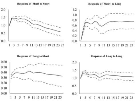
Figure 7 shows impulse response functions from a VAR containing the short- and long-term interest rates. In response to a 1 percentage-point rise in the policy rate, the long-term rate initially rises 0.36 percentage points. The response declines gradually but is statistically significant the whole 24 months. Figure 8 contains impulse response functions calculated from estimates with CPI inflation rate added to the system.18 The estimated response of the long-term rate to the policy rate is similar to that in Figure 7. Both the short- and long-term rates respond positively to the inflation rate but the response is
FIGURE 10 Coefficient of long-term interest rate to short-term interest rate (1953–92) [Colour figure can be viewed at wileyonlinelibrary.com]
significant only for the long-term rate. The response of the short rate to the long rate does not change much when the inflation rate is added to the system.
Figure 9 repeats the exercise in Figure 7 for the Bretton Woods years. The impulse response for this sub-period shows a smaller response of the long-term rate to the policy rate than for the whole 1952–92 period. The response is, however, statistically significant and above 0.15 percentage points throughout the 24-month period.
6.3
|
Rolling regressions
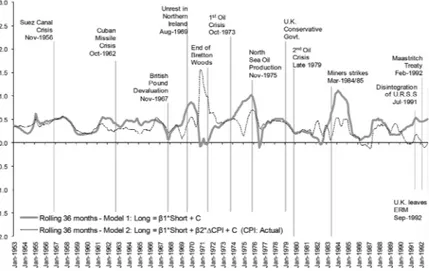
Regressions are estimated for rolling 36-month intervals. We estimate a regression of the long rate on the short rate and another adding the CPI inflation rate. Figure 10 plots the coefficient on the policy rate in these regressions over the years 1953–92. The figure also shows the dates of events that might have been sources of financial instability.
The chart shows that responses of the long-term rate to the policy rate are on average much larger than those for the Gold Standard regime. The response of the long-term rate to the policy rate was more volatile in the flexible exchange rate years. There is also a pattern of higher responses in a number of crisis periods. Adding the inflation rate to the rolling regression reduces variation in the coefficient on the short rate but does not change its general pattern.
7
|
INFLATION TARGETING: 1992
–2013
Inflation targeting began with Chancellor of the Exchequer Norman Lamont’s speech in October 1992. The first Bank of England Inflation report followed in February 1993. There were other steps in the evolution of inflation targeting, most notable the granting of operational independence to the Bank of England in May 1997, formalized by the Bank of England Act later that year.19We examine the effect on our estimates of dating the regime change at this later date.
Beginning in early 2009 the policy rate hit its lower bound. Our examination of the inflation targeting regime is confined to 1992–2008.
7.1
|
The transmission mechanism
The theory behind inflation targeting is the New Keynesian model (Svensson, 2011; Woodford, 2003, 2011). A central relationship in the model is the forward-looking Phillips Curve
πt¼ Etπtþ1þ αγtþ ut ð2Þ
whereπ is the inflation rate, y is the output gap, u is a productivity shock, and Etdenotes the rational
expectations operator. Inflation targeting influences actual inflation by managing inflationary expectations.
Monetary policy also operates by controlling the output gap via the short-term interest rate. This channel can be seen from an equation termed the IS equation:
yt¼ artþ bEtytþ c ð3Þ
where r is the short-term interest rate which is‘under the control of the central bank’ and c is a constant term.
The model appears to place the New Keynesians in the camp of the‘short-enders’. The issue is, however, complex. If policy is conducted under commitment, there will be policy effects on the expected future path of short-term rates. These expectations effects are important in stabilizing inflationary expectations in Eq. (2) and via the expected future income term in Eq. (3).20Can the model allow for the Keynes Effect? The New Keynesian model is typically interpreted with‘income’ as total household expenditure. Woodford (2003, chapter 5) extends the model to explicitly include endogenous capital formation. In the extended model investment depends on an expected‘very long real rate’.21
FIGURE 11 Inflation targeting (1992–2008): interest rates [Colour figure can be viewed at wileyonlinelibrary.com]
FIGURE 12 Inflation targeting (1997–2008): interest rates [Colour figure can be viewed at wileyonlinelibrary.com]
Within these two forward-looking versions of the model, monetary policy does affect the long-term interest rate. The regime anchors long-long-term inflationary expectations and thus long-long-term interest rates; a credible reaction function for the policy rate implements the regime. Additional changes in the policy rate (shocks in VARs) will, however, have smaller effects in a regime of
FIGURE 13 Coefficient of long-term interest rate to short-term interest rate (1992–2009) [Colour figure can be viewed at wileyonlinelibrary.com]
well-anchored inflationary expectations. This is the converse of Bernanke’s view that ‘high sensitivity of long-term interest rates to Fed actions suggests some uncertainty about the Fed’s long-run inflation target’.
Additionally, in his New Keynesian model, Woodford resurrects Wicksell’s concept of a natural (or neutral) interest rate.
Keynes (1936) abandoned the natural rate concept. He found its definition problematic in the model of The general theory in which a saving-investment equilibrium could occur at a different natural rate for each level of equilibrium output (p. 242). Woodford (2003, p. 238) argues that‘inflation and output determination can be usefully explained in Wicksellian terms—as depending on the relation between a natural rate of interest determined by real factors and the central bank’s rule adjusting the short-term nominal interest rate that serves as its operating target’.
The natural rate in Woodford’s framework is the rate that stabilizes the price level (or inflation rate) with the output gap at zero. Woodford’s natural rate is, however, stochastic, depending on shocks to government purchases, productivity, time preference, labour supply, and other exogenous disturbances. It may also be negative at times. How the natural rate can figure in design of current monetary policy is a question we return to in the conclusion.
7.2
|
VAR analysis
Figure 11 shows impulse responses for the two-variable VAR containing the long- and short-term interest rates for October 1992–December 2008. Figure 12 shows estimates with the alternate starting date of May 1997.
Figure 11 indicates that a 1 percentage-point rise in the policy rate initially increases the term rate. The effect is statistically significant for three months. The response of the long-term rate then becomes negative and significant with a rather wide confidence interval for the remainder of the 24-month period. With the 1997 starting point (Figure 12), the initial response is also positive, lasting eight months. After this, the response cycles between negative and positive but is insignificant. This pattern is in contrast to the 1952–92 period (Figure 7) where the effect of the policy rate on the long-term rate is positive and significant for the whole 24-month period.22
We also estimated a three-variable VAR for each dating of inflation targeting that adds the CPI inflation rate. The impulse responses of the long-term rate to the policy rate are similar to that in the two-variable case.
7.3
|
Rolling regressions
Figure 13 shows coefficients from rolling regressions of the long-term rate on the short-term rate and from a regression which adds the CPI inflation rate. The rolling regressions are for 36-month samples from January 1992 to December 2009. Estimated responses of long rates to policy actions under inflation targeting are quite different from those for 1952–92. Beginning with the adoption of inflation targeting, the estimated coefficients decline gradually from 0.5 to zero by the beginning of 1997. Following the granting of operational independence to the Bank of England, the coefficient is negative for two to three years and oscillates between positive and negative values thereafter.
For 1997–2000, the negative coefficients reflect the fact that during these years a rise in the policy rate was accompanied by a fall in the long-term rate. Gordon Brown announced Bank of England operational independence on 6 May 1997. Independence was formalized by legislation effective as of 1 June 1998. A plausible explanation is that as the regime gained credibility, inflationary expectations became better anchored and the long-term interest rate fell.
8
|
CONCLUSIONS
Figure 14 shows impulse responses for the effect of Bank Rate (or another policy rate) on the long-term rate for each of four policy regimes. R. G. Hawtrey was born in 1879 and would have taken it for granted that in times of peace long-run inflationary expectations were anchored by the Gold Standard. Given the limited goals of monetary policy in that regime, changes in Bank Rate would have been expected to be temporary and have little effect on the rate on Consols. The transmission mechanism was via the short-term rate: the Hawtrey Effect.
Keynes worked during the interwar years, an era of much less certainty about long-term inflation. Keynes believed that there were significant effects on long-term rates from changes in Bank Rate. His view of the transmission mechanism was one where changes in the long rate affected fixed investment: the Keynes Effect. Our results (Sections 4 and 5) support both Hawtrey and Keynes.
For nearly a half century following World War II, although there was less monetary uncertainty than during the interwar years, our results indicate no return to the level of anchored inflationary expectations that existed under the classical Gold Standard. During these years, changes in Bank Rate (or another policy rate) continued to have significant sustained effects on the long-term interest rate (Figures 7–9): The Keynes Effect was operative. The goals of monetary policy had become more complex; policy was by discretion and whether changes in Bank Rate would be maintained depended, as Hicks put it, on whether the public believed that the Bank ‘means business’.
The move to inflation targeting in the 1990s was a regime shift aimed at anchoring long-term inflationary expectations. One predicted effect of inflation targeting was to make the long-term interest rate ‘jump around a bit less’ in response to short-run nominal disturbances including changes in the monetary policy rate. Our results are consistent with success in this regard (Figures 11–13).
In recent years the zero-bound problem has limited the effectiveness of policy rates. Central banks have turned to instruments such as forward guidance, purchases of long maturity assets, and subsidies to bank lending to influence longer-term rates. Our analysis suggests that such measures may be needed in normal times as well if monetary policy is to affect long-term rates in a regime of well-anchored run inflationary expectations. While a credible inflation targeting regime lends stability to long-term rates, it limits the effect of changes in the policy rate to combat disturbances to the economy. Turner (2011) asks whether the long-term interest rate is a‘policy victim, policy variable or policy lodestar?’ It has become a policy variable to some central banks, a variable the control of which may require instruments in addition to the policy rate.23
Moreover, as central banks move to normalize interest rates, the issue of the natural (or neutral) interest rate returns.24 Woodford (2003) resurrects the concept in the New Keynesian model but application to real-world policy raises difficult questions not the least of which is measurement.
ENDNOTES
1Rogoff, Kenneth (2005, 23 April), A case for financial transparency. Financial Times, p. 13.
2Bernanke cites Gürkaynak et al. (2005) for evidence that under Federal Reserve procedures at the time, the views of
long-run inflation of ‘private agents’ were not strongly anchored. Gürkaynak et al. (2010) find that inflationary
expectations were more firmly anchored in the United Kingdom under inflation targeting.
3Sample periods in this section end with December 2008. In early 2009, the short-term rate was fixed at 0.5%.
4See Appendix B (available online at the publisher’s website) for these results.
5See Sims, Stock, and Watson (1990) and Lutkepohl and Reimers (1992).
6For the classical Gold Standard period, we also estimate a VAR with the level of Bank of England gold reserves as an
additional variable placed last in the ordering.
7Estimates of Eq. (1) expanded by coefficient dummy variables for each sub-period are reported in Appendix B,
available online. The estimated coefficient dummies indicate that relative to the Gold Standard period,β1in Eq. (1) is
higher in each of the other periods.
8This pattern is followed in all figures showing impulse response functions with the exception of Figure 2, which shows
impulse responses across different VAR specifications without confidence bands. Confidence bands are calculated using Monte Carlo methods with 2,500 draws. A one-unit shock, rather than a one-standard deviation shock, is used for comparability across regimes.
9CPI inflation is used for comparability with later periods. Because monthly data are available only post-World War I,
monthly observations are interpolated from annual data.
10Additional sources are listed in Appendix A, available online.
11There is spike in the coefficient in 1895 when a border conflict between Venezuela and British Guiana led President
Cleveland to threaten war if Britain refused US mediation. The threat coincided with the Kruger telegram from the
German Kaiser expressing support for the Boers in Transvaal. See Trevelyan (1937, pp. 418–419).
12On these issues, see Hicks (1967, chapters 9–11), Patinkin (1976, chapters 3–8), and Harrod (1969, chapter 7).
13Hicks, Harrod, and Robertson criticize Keynes for dropping the natural rate concept. Hicks sees it as‘leaving the
interest rate hanging by its own bootstraps;’ Robertson as leaving a ‘grin without a cat’ (Harrod, 1969, p. 175).
14Impulse responses were also calculated from VARs with WPI inflation. The response of the Consol rate to Bank Rate is
similar to those in Figures 4 and 5. The peak effect lies between that in the two figures.
15The sample starts in 1952 to avoid years characterized by a devaluation of the pound and controls of the economy.
Moreover, Bank Rate remained at 2% until November 1951.
16See Gurley (1960, p. 674).
17See Roosa (1951) and Goodhart (1989, chapter 12).
18We also estimate a three-variable VAR with WPI inflation. Impulse responses from that system show a response of the
long rate to the policy rate similar to those in Figure 8.
19Inflation targeting in the United Kingdom is described in King (1997) and Bean and Jenkinson (2001).
20In the backward-looking version of the New Keynesian model (Ball, 1999), the current short-term interest rate is the
only channel for monetary policy.
21In Ravenna and Walsh (2006), monetary policy works via a cost channel. The short-term interest rate affects cost of
production because the wage bill is financed by borrowing. This is the Hawtrey Effect via working rather than liquid capital.
22Hawtrey and Keynes would have expected a positive response of the long-term rate to a rise in the policy rate. Romer
(2012, p. 521), within a rational expectations framework, argues that a negative response is‘intuitive’.
23In September 2016, the Bank of Japan adopted a strategy of targeting the 10-year bond rate via sales and purchases of
long-term bonds.
REFERENCES
Ball, L. (1999). Efficient rules for monetary policy. International Finance, 2, 63–83.
Barsky, R. B. (1987). The Fisher hypothesis and the forecastability and persistence of inflation. Journal of Monetary
Economics, 19, 3–24.
Bean, C. R., & Jenkinson, N. H. (2001). The formulation of monetary policy at the Bank of England. Bank of England
Quarterly Bulletin, 41, 434–441.
Benati, L. (2004). Evolving post-World War II UK economic performance. Journal of Money, Credit and Banking, 36,
691–717.
Bernanke, B. (2004). Inflation targeting. Federal Reserve Bank of Saint Louis Review, 86, 165–168.
Chadha, J. S., & Perlman, M. (2014). Was the Gibson paradox for real? A Wicksellian study of the relationship between
interest rates and prices. Financial History Review, 21, 139–163.
Chadha, J. S., and Sarno, L. (2002). Short- and long-run price level uncertainty under different monetary policy regimes:
An international comparison. Oxford Bulletin of Economics and Statistics, 64, 187–216.
Cogley, T., Sargent, T. J., & Surico, P. (2015). Price-level uncertainty and instability in the United Kingdom. Journal of
Economics and Control, 52, 1–16.
Friedman, M., & Schwartz, A. (1982). Monetary trends in the United States and United Kingdom. Chicago, IL: University of Chicago Press.
Goodhart, C. A. E. (1989). Money, information and uncertainty (2nd ed.). Cambridge, MA: MIT Press.
Gürkaynak, R., Levin, A., & Swanson, E. (2010). Does inflation targeting anchor long-run inflation expectations?
Evidence from the US, UK, and Sweden. Journal of the European Economic Association, 8, 1208–1242.
Gürkaynak, R., Sack, B., & Swanson, E. (2005). The sensitivity of long-term interest rates to economic news: Evidence
and implications for macroeconomic models. American Economic Review, 95, 425–436.
Gurley, J. (1960). The Radcliffe report and evidence. American Economic Review, 50, 672–700.
Hamilton, J., Harris, E., Hatzius, J., & West, K. (2015). The equilibrium real funds rate: Past, present and future. NBER Working Paper 21476.
Harrod, R. (1969). Money. London: Macmillan.
Hawtrey, R. G. (1938). A century of Bank Rate. London: Longmans. Hicks, J. (1939). Value and capital. London: Oxford University Press. Hicks, J. (1946). Value and capital (2nd ed.). London: Oxford University Press. Hicks, J. (1967). Critical essays in monetary theory. London: Oxford University Press.
Jennrich, R. (1970). An asymptoticχ2test for the equality of two correlation matrices. Journal of the American Statistical
Association, 65, 904–1012.
Keynes, J. M. (1930). A treatise on money. London: Macmillan.
Keynes, J. M. (1936). The general theory of employment, interest, and money. New York: Harcourt Brace.
King, M. A. (1997). The inflation target five years on. Bank of England Quarterly Review, 37, 434–442.
Lutkepohl, H., & Reimers, H. (1992). Impulse response analysis of co-integrated systems. Journal of Economic
Dynamics and Control, 16, 53–78.
Mankiw, N. G., Miron, J. A., & Weil, D. N. (1987). The adjustment of expectations to a change in regime: A study of the
founding of the Federal Reserve. American Economic Review, 77, 358–374.
Overy, R. (2009). The twilight years: The paradox of Britain between the wars. London: Penguin Books.
Patinkin, D. (1976). Keynes’ monetary theory. Durham, NC: Duke University Press.
Ravenna, F., & Walsh, C. E. (2006). Optimal monetary policy with the cost channel. Journal of Monetary Economics, 53,
199–216.
Robertson, D. H. (1937). Review: A century of Bank Rate. by R. G. Hawtrey. Economic Journal, 44, 94–96.
Romer, D. (2012). Advanced macroeconomics (4th ed.). New York: McGraw Hill.
Roosa, R. V. (1951). Interest rates and the central bank. In L. Dupriez (Ed.), Money, interest and growth. New York: Macmillan.
Sims, C. A., Stock, J. H., & Watson, M. W. (1990). Inference in linear time series models with unit roots. Econometrica,
58, 113–144.
Svensson, L. (2011). Inflation targeting. In B. M. Friedman & M. Woodford (Eds.), Handbook on monetary economics. Amsterdam: Elsevier.
Turner, P. (2011). Is the long-term interest rate a policy victim, a policy variable or a policy lodestar? BIS Working Paper No. 367.
Woodford, M. (2003). Interest and prices. Princeton, NJ: Princeton University Press.
Woodford, M. (2011). Optimal monetary stabilization policy. In B. M. Friedman & M. Woodford (Eds.), Handbook on monetary economics. Amsterdam: Elsevier.
SUPPORTING INFORMATION
Additional supporting information may be found in the online version of this article at the publisher's web-site.
How to cite this article:Berument H, Cabezon E, Froyen R. A century and three-quarters of Bank Rate and long-term interest rates in the United Kingdom. International Finance. 2017;20:26–47. https://doi.org/10.1111/infi.12101
![FIGURE 1 Classical gold standard period (1844 –1913): interest rates [Colour figure can be viewed at wileyonlinelibrary.com]](https://thumb-eu.123doks.com/thumbv2/9libnet/5625111.111512/7.727.128.601.601.936/figure-classical-standard-period-colour-figure-viewed-wileyonlinelibrary.webp)
![FIGURE 3 Coefficient long-term interest rate to short-term interest rate (1844 –1915) [Colour figure can be viewed at wileyonlinelibrary.com]](https://thumb-eu.123doks.com/thumbv2/9libnet/5625111.111512/8.727.127.598.70.259/figure-coefficient-long-short-colour-figure-viewed-wileyonlinelibrary.webp)
![FIGURE 4 Interwar years (1919 –33): interest rates [Colour figure can be viewed at wileyonlinelibrary.com]](https://thumb-eu.123doks.com/thumbv2/9libnet/5625111.111512/10.727.127.601.618.957/figure-interwar-years-rates-colour-figure-viewed-wileyonlinelibrary.webp)
![FIGURE 6 Coefficient long-term interest rate to short-term interest rate (1920 –33) [Colour figure can be viewed at wileyonlinelibrary.com]](https://thumb-eu.123doks.com/thumbv2/9libnet/5625111.111512/11.727.120.601.65.410/figure-coefficient-long-short-colour-figure-viewed-wileyonlinelibrary.webp)
![FIGURE 9 Fixed exchange rate regime (1952:1 –1973:2): interest rates [Colour figure can be viewed at wileyonlinelibrary.com]](https://thumb-eu.123doks.com/thumbv2/9libnet/5625111.111512/13.727.120.601.63.374/figure-fixed-exchange-regime-colour-figure-viewed-wileyonlinelibrary.webp)