ALGORITHMS FOR EFFECTIVE
QUERYING OF GRAPH-BASED PATHWAY
DATABASES
a thesis
submitted to the department of computer engineering
and the institute of engineering and science
of bilkent university
in partial fulfillment of the requirements
for the degree of
master of science
By
Ahmet C
¸ etinta¸s
July, 2007
I certify that I have read this thesis and that in my opinion it is fully adequate, in scope and in quality, as a thesis for the degree of Master of Science.
Assoc. Prof. Dr. U˘gur Do˘grus¨oz(Advisor)
I certify that I have read this thesis and that in my opinion it is fully adequate, in scope and in quality, as a thesis for the degree of Master of Science.
Prof. Dr. ˙Ismail Hakkı Toroslu
I certify that I have read this thesis and that in my opinion it is fully adequate, in scope and in quality, as a thesis for the degree of Master of Science.
Asst. Prof. Dr. Ali Aydın Sel¸cuk
Approved for the Institute of Engineering and Science:
Prof. Dr. Mehmet B. Baray Director of the Institute
ABSTRACT
ALGORITHMS FOR EFFECTIVE QUERYING OF
GRAPH-BASED PATHWAY DATABASES
Ahmet C¸ etinta¸s
M.S. in Computer Engineering
Supervisor: Assoc. Prof. Dr. U˘gur Do˘grus¨oz July, 2007
As the scientific curiosity shifts toward system-level investigation of genomic-scale information, data produced about cellular processes at molecular level has been accumulating with an accelerating rate. Graph-based pathway ontologies and databases have been in wide use for such data. This representation has made it possible to programmatically integrate cellular networks as well as investigating them using the well-understood concepts of graph theory to predict their struc-tural and dynamic properties. In this regard, it is essential to effectively query such integrated large networks to extract the sub-networks of interest with the help of efficient algorithms and software tools.
Towards this goal, we have developed a querying framework along with a num-ber of graph-theoretic algorithms from simple neighborhood queries to shortest paths to feedback loops, applicable to all sorts of graph-based pathway databases from PPIs to metabolic pathways to signaling pathways. These algorithms can also account for compound or nested structures present in the pathway data, and have been implemented within the querying components of Patika (Pathway Analysis Tools for Integration and Knowledge Acquisition) tools and have proven to be useful for answering a number of biologically significant queries for a large graph-based pathway database.
Keywords: Graph Algorithms, Graph Querying, Biological Pathways, Pathway Databases.
¨
OZET
C
¸ ˙IZGE TABANLI YOLAK VER˙I TABANLARININ
ETK˙IN SORGULANMASI ˙IC
¸ ˙IN ALGOR˙ITMALAR
Ahmet C¸ etinta¸s
Bilgisayar M¨uhendisli˘gi, Y¨uksek Lisans Tez Y¨oneticisi: Do¸c. Dr. U˘gur Do˘grus¨oz
Temmuz, 2007
Bilimsel merak, kalıtım-¨ol¸cekli bilginin sistem seviyesindeki ara¸stırmalarına y¨onelirken, molek¨ul d¨uzeyindeki h¨ucresel s¨ure¸cler hakkında ¨uretilen veriler hızlanan bir oranla artmaktadır. C¸ izge tabanlı yolak ontolojiler ve veri tabanları bu tarz bilgiler i¸cin geni¸s bir kullanım alanına sahiptir. Bu g¨osterim, h¨ucresel a˘gların programlı bir ¸sekilde b¨ut¨unle¸stirilmesinin yanı sıra yapısal ve dinamik ¨
ozelliklerini tahmin etmeye y¨onelik olarak ¸cizge teorinin iyi anla¸sılmı¸s kavramları kullanılarak ara¸stırılmasını m¨umk¨un kılmaktadır. Bu kapsamda, b¨oyle b¨ut¨unle¸sik geni¸s a˘gların, ilgili alt-a˘gların etken algoritmalar ve yazılım ara¸clarının yardımıyla se¸cilerek ¸cıkarılması amacıyla, etkili olarak sorgulanması zaruridir.
Bu ama¸cla, protein-protein etkile¸siminden, metabolik yolaklara hatta sinyal yolaklarına her t¨url¨u ¸cizge tabanlı yolak veri tabanlarına uygulanabilir olmak ¨
uzere, basit kom¸suluk sorgularından en kısa yol yolaklarına ve geri besleme d¨ong¨ulerine pek ¸cok ¸cizge teorik algoritmalar beraberinde bir sorgulama ¸cer¸cevesi geli¸stirdik. Bu algoritmalar ayrıca yolak veritabanı i¸cinde mevcut bile¸sik veya birbirinin i¸cine yerle¸stirilmi¸s yapıları da olu¸sturulabilir ve Patika (Entegrasyon ve Bilgi Kazanma i¸cin Yolak Analiz Ara¸cları) yazılımlarının sorgulama unsurları i¸cerisinde uygulanmı¸stır. Ayrıca, s¨ozkonusu algoritmaların geni¸s bir ¸cizge tabanlı yolak veritabanı i¸cin biyolojik olarak ¨onem arz eden pek ¸cok sorgunun cevap-landırılması i¸cin kullanı¸slı oldu˘gu g¨or¨ulm¨u¸st¨ur.
Anahtar s¨ozc¨ukler : C¸ izge Algoritmaları, C¸ izge Sorgulama, Biyolojik Yolaklar, Yolak Veri Tabanları.
Acknowledgement
I would like to express my deepest gratitude to my supervisor Assoc. Prof. U˘gur Do˘grus¨oz for his invaluable support, continuous encouragement and incred-ible effort in the supervision of the thesis. It was a wonderful opportunity to work with him.
I would like to thank Prof. Dr. ˙Ismail Hakkı Toroslu and Asst. Prof. Dr. Ali Aydın Sel¸cuk for accepting to read and review the thesis.
I wish to thank Emek Demir and ¨Ozg¨un Babur for their constructive and critical comments. I also wish to thank C¸ a˘grı Aksay, G¨ozde C¸ ¨ozen, C¸ a˘gatay Bilgin, Hilmi Yıldırım, Hande K¨u¸c¨uk and Serhat Tekin for their contributions. I wish to thank all other members of PATIKA team. It was a great experience to be a member of such a friendly team.
Finally, a special thank goes to my wife ¨Oznur for her encouragement, support and patience in every step of my study.
This thesis was supported by TUBITAK (Scientific and Technical Research Council of Turkey) with National Scholarship Programme for MSc Students.
Contents
1 Introduction 1
1.1 Motivation . . . 1
1.2 Contribution . . . 3
1.3 Organization of the Thesis . . . 4
2 Theory and Background 5
2.1 Preliminary Definitions . . . 5
2.2 Graph Representation of Pathways . . . 6
2.3 Patika Architecture . . . 7 3 Related Work 9 4 Method 12 4.1 Neighborhood . . . 12 4.2 Graph of Interest . . . 13 4.3 Common Regulation . . . 17 vi
CONTENTS vii
4.4 Shortest Path . . . 19
4.5 Feedback . . . 22
4.6 Stream . . . 25
4.7 Subgraph Matching . . . 27
4.8 Compound Structures & Ubiquitous Entities . . . 28
5 Implementation 30 5.1 Patika . . . 30
5.1.1 Model Layer . . . 30
5.1.2 Concrete Implementations . . . 30
5.1.3 Patika Graphs and Excision Support . . . 32
5.1.4 Patika Server Architecture . . . . 33
5.1.5 Clients . . . 34
5.2 Patika Query Framework . . . 34
5.2.1 Query Structures . . . 35
5.2.2 Query Execution and Data Flow . . . 44
5.2.3 Query User Interface . . . 50
5.2.4 Query Framework Deployment . . . 71
6 Test Results and Performance 75
List of Figures
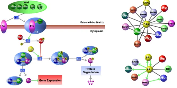
1.1 Sample pathways represented by Patika ontology. (left) Canoni-cal wnt pathway containing examples of compound structures such as regular abstractions (e.g. “protein degradation”), homology abstractions (e.g. 5 wnt genes), and molecular complexes (e.g. APC:Axin). (right) Partial human interaction networks contain-ing PPIs and transcriptional regulation interactions of proteins CRK and SP1, respectively. . . 2
1.2 Conceptual illustration of how pathways are assumed to be already integrated in the knowledgebase (bottom part, where each pathway is color-coded uniquely), which is typically on disk, and how the sub-network of interest (parts of three different original pathways) may be extracted and presented to the user as a result of a query. 3
4.1 2-neighborhood (yellow) of proteins SCH1 and PTEN (green) in a partial PPI network. Notice that only the edges leading to these neighbors (i.e. visited during traversal) are highlighted. . . 13
4.2 (upper-left) A PPI network with proteins of interest CRK and CRKL (green); (upper-right) Graph of interest (yellow) formed by using paths of length up to 3 (k = 3) between nodes of interest (green); (bottom) Graph of interest with k = 2 (k = 1 returns no results). . . 14
LIST OF FIGURES ix
4.3 Common regulators, with path limit 2, of small molecules contain-ing the word “lauro” in their name (cyan) in this partial mechanis-tic pathway are found to be a single node representing a molecular complex (green). The paths from the common regulator to the target nodes are highlighted (yellow). . . 18
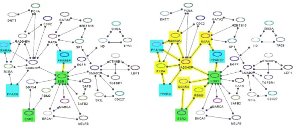
4.4 Shortest paths (yellow) between bioentities whose names start with “PPA” (cyan) and those whose names contain “ESR” (green) with (left) d = 0 and (right) d = 2. Notice that the length of a shortest path between these two node sets is k = 2. . . 19
4.5 Positive feedback (yellow) of a specified Citrate state in mitochon-dria (green) with up to length 10; the result contains two feedback cycles, one in mitochondria (of length 10) and one through cyto-plasm (of length 8). . . 22
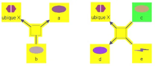
4.6 (left) Up (green) and down (cyan) stream of protein “a” (yellow) in a partial mechanistic pathway. (right) Unambiguous positive upstream of node “a” (yellow) contains node “b” (green) only, as node “c” is on both positive and negative paths leading to node “a”. 26
4.7 Traversal reaching complex “c1” from the transition on the left will continue to transition on the right if and only if “Link Members of Complex” option is true. . . 29
4.8 Whether or not state “a” is in the 4-neighborhood (green) of state “c” (yellow) depends on whether traversal over ubiques (“ubique x” in this case) is allowed. Obviously, in this case it is allowed. . . 29
5.1 Class hierarchy of the primary Patika objects. . . . 31
5.2 The class diagram of field query nodes. A composite pattern was used for arbitrary nesting of query objects. . . 37
LIST OF FIGURES x
5.3 General state diagram of FieldQueryParser, for parsing the
Patika query languages field queries. . . 37
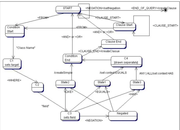
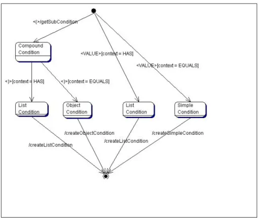
5.4 State diagram of the FieldQueryParser, for deciding on which condition to create. Through composite conditions it is possible to specify arbitrarily nested object relations. . . 38
5.5 Query and Query Result Hierarchy . . . 40
5.6 Query Composition . . . 41
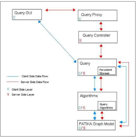
5.7 Data Flow of Query Framework in Patika . . . 45
5.8 Sequence diagram showing that agent emek is running a server side query . . . 49
5.9 Sample query tree to find the union of 1-neighborhood of the objects on the shortest path from states whose name starts with “Fas” to states whose name starts with “RB” with the shortest path from states whose name starts with “Fas” to states whose name starts with “JNK1” . . . 50
5.10 Mechanistic view of the result of the following sample query: paths-of-interest (yellow) with source of all mechanistic nodes whose names contain “caspase-8” (green) and target for those whose names contain “bax” (cyan) with limit 8; Highlight Legend Di-alog for this query shown on right. . . 51
5.11 The user is asked to agree to run the Patika Query Applet. . . . 52
5.12 The Query Dialog consists of a toolbar (top) and panels for query forest (left) and parameters (right). . . 52
5.13 The source of a Neighborhood query is set through the pop-up menu of its ‘source’ query node. . . 53
LIST OF FIGURES xi
5.14 The user can specify whether the query is to execute on the data-base or the view. . . 53
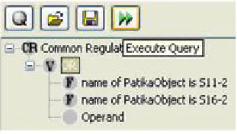
5.15 The query rooted at the OR query is executed when the user presses associated button. . . 53
5.16 Sample Query Result Dialog . . . 54
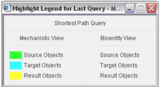
5.17 Sample Query Highlight Legend Dialog, where the last query is a shortest path query, and source, target and result (shortest paths) objects are highlighted with distinct colors (green, cyan and yellow, respectively). . . 54
5.18 You may constrain your query to a Patika object of a specific type. 55
5.19 All states of protein ‘tp53’ (yellow) as obtained by a ‘States of a Bioentity’ query . . . 56
5.20 Sources (yellow) of protein ‘tp53’ (green) as obtained by a ‘Sources of a Bioentity’ query . . . 56
5.21 Products (yellow) of DNA ‘tp53’ (green) as obtained by a ‘Products of a Bioentity’ query . . . 57
5.22 Queries can be combined through logical operators: Search for all PatikaNode’s whose description contains ‘colon cancer’ or ID equals 3835 authored by Joe Smith. . . 57
5.23 Advanced Query Options Dialog is used to set traversal options for ubiques and abstractions. . . 58
5.24 Whether or not ‘a’ is in the 4-neighborhood (green) of ‘c’ (yellow) depends on whether traversal over ubiques (‘ubique x’ in this case) is allowed. Obviously, in this case it is allowed. . . 58
5.25 Sample Neighborhood Query Dialog for 1-neighborhood of protein bioentities whose names start with ‘crk’ . . . 59
LIST OF FIGURES xii
5.26 1-neighborhood of protein bioentities whose names start with ‘crk’ (result of the query in Figure 5.25) . . . 59
5.27 Immediate neighbors (yellow) of protein ‘CRKL’ (green) may be queried using its popup menu . . . 60
5.28 Sample GoI Query Dialog . . . 60
5.29 Result of the query in Figure 5.28: GoI (yellow) of protein bioen-tities whose names start with ‘crk’ (cyan) where limit is 3 (left) and where limit is 2 (right). Notice that each protein on the GoI (yellow) is on at least one path between two source nodes (cyan) whose length is at most limit. . . 61
5.30 Sample PoI Query Dialog . . . 61
5.31 Result of the query in Figure 5.30: PoI (yellow) between mech-anistic nodes whose names contain ‘caspase-8’ (green) and those whose names contain ‘bax’ (cyan) . . . 62
5.32 Sample Common Regulator Query Dialog . . . 62
5.33 Result of the sample common regulator query in Figure 5.32, where we find common regulators (green) of the simple states whose names contain ‘lauro’ (cyan); paths leading from common regu-lators to the targets are shown in yellow. . . 63
5.34 Sample Shortest Paths Query Dialog . . . 64
5.35 Result of the sample shortest paths query in Figure 5.34, where we find directed shortest paths (yellow) from simple states whose names contain ‘caspase’ (green) to simple states whose names con-tain ‘bad’ (cyan) . . . 65
LIST OF FIGURES xiii
5.37 Result of the sample feedback query in Figure 5.36, where we look for positive feedback (yellow) of a given Citrate state (with spec-ified ID) in mitochondria (green) with up to length 10; the result contains two feedback cycles, one in mitochondria (of length 10) and one through cytoplasm (of length 8). . . 66
5.38 Sample Stream Query Dialog . . . 66
5.39 Result of the sample stream query in Figure 5.38, where we look for unambiguous positive upstream, with limit 4, (yellow) of complexes whose names start with ‘active caspase’ (green) . . . 67
5.40 Query for simple states whose name starts with ‘FASL’ . . . 68
5.41 Result (yellow) of the FAS Ligand query in Figure 5.40 . . . 68
5.42 Query for Caspase complexes, which does not contain words ‘pre-cursor’, ‘pro-caspase’ or ‘procaspase’ . . . 69
5.43 Result (green) of Caspase query in Figure 5.42 added to the exist-ing model . . . 69
5.44 Shortest path query using the previous queries as source and target; the query limits the distance to 5 and considers directions. . . 70
5.45 Result of the shortest path query in Figure 5.44; we find that the two shortest paths (yellow) from FAS Ligand (green) to Caspase complexes (cyan) goes to Caspase-8 dimer in cytoplasm, each with 2 transitions (4 steps). . . 70
5.46 Shortest path query with further distance set to 8 . . . 71
5.47 Result of the shortest path query in Figure 5.46. Paths of length up to 12 (yellow) are found between source (green) and target (cyan) sets, since the shortest path length is 4. . . 72
LIST OF FIGURES xiv
5.48 A GoI query where the previous FAS Ligand and Caspase complex queries are gathered into an OR query and used as seed (molecules
of interest) . . . 72
5.49 Result of the GoI query in Figure 5.48 . . . 73
5.50 Deployment Diagram of Query Framework in Patika . . . 74
6.1 Result set size vs. execution time for GoI algorithm . . . 76
6.2 Distance (k) vs. execution time for GoI algorithm for various source set sizes (|S|) . . . 76
6.3 Shortest length vs. total execution time of the shortest-path algo-rithm . . . 77
6.4 Distance (k) vs. execution time for CR algorithm for various source set sizes (|S|) . . . 78
6.5 Distance (k) vs. execution time for Stream algorithm for various source set sizes (|S|) . . . 78
Chapter 1
Introduction
1.1
Motivation
Human genome is expected to create an extremely complex network of informa-tion, composed of hundred thousands of different molecules and factors [3, 18]. Knowing the exact map of this network is very important since it will poten-tially explain the mechanisms of life processes as well as disease conditions. Such knowledge will also serve as a key for further biomedical applications such as de-velopment of new drugs and diagnostic approaches. In this regard, a cell can be considered as an inherently complex multi-body system. In order to make useful deductions about such a system, one needs to consider cellular pathways as an interconnected network rather than separate pathways.
Our knowledge about cellular processes is increasing at a rapidly growing pace. Novel large scale analysis methods are already applied to yeast to provide data about the yeast proteome [16, 27]. However, most of the time these data are in fragmented and incomplete forms. One of the most important challenges in bioinformatics is to represent and integrate this type of knowledge. Efficient construction and use of such a knowledge base depends highly on a strong on-tology (i.e., a structured semantic encoding of knowledge). This knowledge base then can act as a blueprint for simulations and other analysis methods, enabling
CHAPTER 1. INTRODUCTION 2
us to understand and predict the behavior of a cell much better.
Figure 1.1: Sample pathways represented by Patika ontology. (left) Canon-ical wnt pathway containing examples of compound structures such as regular abstractions (e.g. “protein degradation”), homology abstractions (e.g. 5 wnt genes), and molecular complexes (e.g. APC:Axin). (right) Partial human in-teraction networks containing PPIs and transcriptional regulation inin-teractions of proteins CRK and SP1, respectively.
Conventional approaches for representation of cellular pathways are based on pathway drawings composed of still images. Although easy to create, such draw-ings are often not reusable and the ontologies used are far from being uniform and consistent, highly depending on implicit conventions rather than explicit, formal rules. Recently this has resulted in a major shift in the use of more formal ontologies and dynamic representation of pathways that support programmatic integration and manipulation of pathways regardless of the underlying ontology. Among these, graphs, one of the most common discrete mathematical struc-tures [6], have been most popular for “in-silico” modeling of biological pathways, from metabolic pathways to gene regulatory networks, from proteprotein in-teraction networks to signaling pathways [2, 10, 20, 15]. Such modeling is crucial for the field of systems biology, which deals with a systems-level understanding of biological networks.
CHAPTER 1. INTRODUCTION 3
1.2
Contribution
In this thesis, we present a framework for querying a compound graph-based pathway database as well as a number of graph algorithms needed to implement these graph-based queries. We assume a database in which pathways are stored in an integrated manner, as opposed to a list of independent pathways. Thus, a query to the database is performed over this integrated, higher level (Figure 1.2) network of pathways, and aims to find a sub-network of interest, requiring a rich set of graph algorithms.
Figure 1.2: Conceptual illustration of how pathways are assumed to be already integrated in the knowledgebase (bottom part, where each pathway is color-coded uniquely), which is typically on disk, and how the sub-network of interest (parts of three different original pathways) may be extracted and presented to the user as a result of a query.
This framework and associated graph algorithms have been implemented as part of a new version of the bioinformatics tool Patikaweb [11]. The range of graph-theoretic queries described as part of our framework is among the most comprehensive ones built so far, and to the best of our knowledge, it is the first querying framework taking into account compound structures (i.e. grouping of or abstractions of biological objects to an arbitrary level of depth) in a graph-based knowledgebase.
CHAPTER 1. INTRODUCTION 4
1.3
Organization of the Thesis
The thesis is organized as follows: Chapter 2 introduces background information on graphs, use of graphs representing pathways and an overlook to the Patika system. Chapter 3 summarizes the studies in the literature on pathway querying and similar graph algorithms on pathway databases. In Chapter 4, the approach and the algorithms that are developed for pathway analysis are described. Chap-ter 5 includes the software architecture that is implemented in the Patika system. In Chapter 6, execution times of all algorithms implemented are discussed and results are given. Finally, Chapter 7 concludes the thesis.
Chapter 2
Theory and Background
2.1
Preliminary Definitions
Let G = (V, E) be a graph with a non-empty node set V and an edge set E. An edge e = {x, y} or simply xy joining nodes x and y is said to be incident with both x and y. Node x is called a neighbor of y and vice versa.
A path between two nodes n0 and nk is a non-empty graph P = (V, E) with
V = {n0, n1, . . . , nk} and E = {n0n1, n1n2, . . . , nk−1nk}, where ni are all distinct.
n0 and nk are called the end points of path P . Therefore, we can write P as an
ordered set of nodes P = n0n1. . . nk. The length of a path P denoted by |P | is
the number of edges on the path.
A path is said to be directed if all its ordered edges are directed in the same direction. A directed path P is called an incoming (outgoing) path of node n if P ends at target (starts at source) node n.
A directed path is called positive (negative) if it contains an even (odd) number of inhibitors (i.e. inhibition edges).
An incoming (outgoing) path of a node is a directed path ending at (starting with) that node.
CHAPTER 2. THEORY AND BACKGROUND 6
Let A and B be set of nodes. Then an A-B path is a path with its ends in A and B, respectively, and no node of P other than its ends is from either set A or B. An A-path is a path where one of the end nodes is from vertex set A, and no other nodes and interactions are from set A.
A path C with identical end nodes is called a cycle.
A directed cycle is called positive feedback (negative feedback) if it contains an even (odd) number of inhibitors.
The distance between dG(x, y) between two nodes x and y in graph G is the
length of a shortest x-y path in G.
If G0 = (V0, E0) is a subgraph of G = (V, E), and G0 contains all the edges xy ∈ E with x, y ∈ V0, then G0 is an induced subgraph of G; we say that V0 induces G0 in G and write G0 = G[V0].
If node x is the starting node of a directed path that ends up at node y, then node y is said to be a target of node x; similarly, node x is said to be a regulator of node y.
2.2
Graph Representation of Pathways
Querying framework and the algorithms described in this thesis have all been de-signed and implemented assuming the Patika ontology [10], which shows utmost similarity to standard representations such as BioPAX [5] and SBGN [22]. How-ever, the results should be able to be applied to most other graph-based pathway representations without difficulty.
Patika ontology is based on a qualitative two-level model. At the entity level, interactions and relations can be addressed in an abstract manner, where the ex-act state of the related parties is unknown, such as protein-protein interex-actions, inferred relations and literature-derived information. At the state/transition or mechanistic level, each entity is associated with a set of states interacting with
CHAPTER 2. THEORY AND BACKGROUND 7
each other via transitions. This level can capture more detailed information such as compartments, molecular complexes and different types of biological events (e.g. covalent modification, transportation and association). This two-level on-tology elegantly covers most biological pathway-related phenomena and is capable of integrating information present in the literature and molecular biology data-bases. Additionally, the Patika ontology uses the notion of compound graphs to represent abstractions, which are logical groupings that may be used to han-dle the complex and incomplete nature of the data. Figure 1.1 shows example pathways drawn at biological entity and state/transition levels.
More formally, a compound pathway graph CG = (G, I) [10] is a 2-tuple of a pathway graph G and a directed acyclic inclusion graph I, where
• V (G) = V is the union of nodes denoting bioentities, states, transitions, molecular complexes, and abstractions of five distinct types: regular, incom-plete state, incomincom-plete transition, homology state, and homology transition; • E(G) is the union of interaction edges of various types (such as PPI edges at bioentity level and activator edges between a state and a transition), some of which are directed;
• V (I) = V (G);
• E(I) is the union of inclusion edges for defining compound structures (mole-cular complexes and abstractions).
In order for a compound pathway graph CG = (G, I) to comply with the Patika ontology, it needs to satisfy certain additional invariants such as regular abstractions cannot have a direct interaction (edge).
2.3
Patika Architecture
Patika is a project of a multi-component environment for cellular pathway data analysis and collaborative construction, which is in progress since 2000. Different
CHAPTER 2. THEORY AND BACKGROUND 8
Patika tools for varying purposes with different user interface have been devel-oped. While Patika 1.0 and Patikapro are standalone applications, Patikaweb serves as a thin client web application. Patikaweb is actually a limited version of Patikapro. Beta version Patika 1.0 beta and Patikaweb 2.1 are released softwares and a professional version Patikapro is currently under development.
Patika has a client-server type architecture. Client side component is a visual editor for pathway construction and analysis. Server side maintains the database where the big picture(i.e., the main repository for pathway data storage) is stored, and coordinates submission process and user communication.
Pathway editor component of Patika is based on Tom Sawyer Software’s1
graph visualization libraries, and implemented using Java technology.
The incorporated graph model is based on Patika ontology. The pathway graph has a two layer representation in the architecture, subject graph and view graphs. Each working instance of the editor has exactly one subject graph, which is a related sub-graph of the database. Multiple number of view graphs may be generated as desired based on a single subject graph.
Chapter 3
Related Work
Graphs have been used in a variety of ways in analyzing cellular networks. In [2] they list three levels of increasing complexity for such analysis, where network topology (global structural properties), interaction patterns (local structural con-nectivity) and network decomposition (hierarchical functional organization) are addressed at each level, respectively. The representation of such complex net-works as graphs has made it possible to investigate the topology and function of these networks using the well-understood concepts of graph theory to predict their structural and dynamic properties or detect special structures or properties in them. In addition, this representation has made the systematic (i.e. program-matic) integration of these complex networks feasible. A comprehensive survey of such prediction, detection and reconstruction methods can be found in [2].
Lately, an extension of this graph representation, namely hierarchically struc-tured graphs or simply compound graphs, where a node of a biological network may recursively contain or include a sub-network of somehow a logically similar group of biological objects [12, 10]. This extension brings in many benefits in modeling, integration, querying and visualization of biological pathways, most important one being reduction of complexity of large networks through decomposition of the network into distinct components or modules.
There is also a great deal of work on querying of occurrences of sub-structures
CHAPTER 3. RELATED WORK 10
(from specified subgraphs to special sub-structures) such as graphlets or motifs in graph-based data, including pathways [2]. Most approaches employ some kind of a graph matching algorithm to find one or all (exact or inexact) instances of the specified subgraph [25, 26, 24]. Yet some others take a comparative approach toward interpreting molecular networks, contrasting and aligning networks of different species and molecular types, and under varying conditions [23].
There exists a heuristic approach in which a merged representation of the two networks being compared is created and then a greedy algorithm is applied for identifying the conserved subnetworks embedded in the merged representation, called a network alignment graph. When there exists a one-to-one correspon-dence between molecules across the two networks, identifying subnetworks in the alignment is simple, however, in general there may be a complex many-to-many correspondence [23, 19].
Use of graph algorithms such as shortest paths between a specified pair of objects in a graph database has been in use for quite a while [14], and their use in graph-based pathway databases have caught attention in recent years [17, 8, 4]. In [14], they define a query language including an operation for finding shortest paths between two simple objects, which are used as the start and target nodes of the search, respectively. Also query has parameter of path type defining a precise structure for the resulting sequence, according to the types of nodes and edges on the path. However, the query language was defined only in fragments, no implementation has been mentioned. Also different path finding and feedback queries are defined for pathway databases in query languages such as PQL [17] and GraphDB [14]. For example, ‘Retrieval of a connected graph that includes a set of specified interactions’ and ‘Retrieval of cycles that include a set of specified interactions’ queries can be expressed, but cannot be computed in PQL, stated as future work.
Path finding in biological networks has some special problems such as highly connected nodes called ubiques. These ubiquitous nodes lead path finding algo-rithms to the irrelevant paths. Therefore two approaches can be applied: first approach is filtering out the selection of these highly connected nodes, and second
CHAPTER 3. RELATED WORK 11
approach is computing the shortest paths on the weighted metabolic graph where each node is assigned a weight equal to its connectivity in the network [8].
Chapter 4
Method
After a careful requirements analysis, we have come up with the following initial set of graph algorithms that might be of use to people querying cellular pathway databases. This set is, by no means, exhaustive, and may easily be extended.
4.1
Neighborhood
One very simple yet quite powerful operation on graphs is finding the neighbors of a specified source node within a certain distance. k-neighborhood of a node set S can be defined as
NB(S, k) = S ∪ {x | x is on an S-path P ∧ |P | ≤ k}
Figure 4.1 explains this operation with an example.
k-neighborhood of a node set can be found by running a regular BFS with the seed taken as the specified source node set. All nodes reached within k iterations are in the resulting neighborhood. This operation takes time linear in the number of neighbors plus the total number of edges incident upon these neighbors.
Biological Significance: Neighborhood query relies on the graph-theoretic ar-gument above, but takes a different point of view. It finds out objects that are
CHAPTER 4. METHOD 13
Figure 4.1: 2-neighborhood (yellow) of proteins SCH1 and PTEN (green) in a partial PPI network. Notice that only the edges leading to these neighbors (i.e. visited during traversal) are highlighted.
closest to the given target(s), thus returns a functional neighborhood(as stated in [9]). This query answers questions like:
• In which pathways does my protein take part?
• With which states does this molecule interact?
• What are the other actors taking part in this process?
• Which proteins catalyze this reaction?
4.2
Graph of Interest
Given a graph G and a set of nodes of interest S (e.g. genes of interest), this operation is to find in G all paths of length at most k between any two nodes of the specified node set. The subgraph of G induced by the nodes of the resulting set gives the graph of interest. More formally,
CHAPTER 4. METHOD 14
Figure 4.2: (upper-left) A PPI network with proteins of interest CRK and CRKL (green); (upper-right) Graph of interest (yellow) formed by using paths of length up to 3 (k = 3) between nodes of interest (green); (bottom) Graph of interest with k = 2 (k = 1 returns no results).
As the name suggests, this operation is aimed at finding a “minimal” subgraph comprising all the nodes of interest complemented by the “missing links” among these nodes. The parameter k defines how long the paths linking nodes of interest to form a graph of interest is allowed to be. Figure 4.2 explains this operation with an example. Below is the pseudo code for this operation. Here two separate BFS are to be run in forward and reverse directions and combined to form a candidate set. The nodes in this candidate set satisfying the maximum path length constraint are put in a result set, which is to be “purified” by a post-processing phase (algorithm purify) during which degree 1 nodes that do not
CHAPTER 4. METHOD 15
lie on paths between source set nodes (effectively subgraphs that are trees in the result set) are pruned.
algorithm GraphOfInterest(S, k)
1 C := GoI-BFS(S, k, f wd) ∪ GoI-BFS(S, k, rev) 2 for q ∈ C do
3 if q.label(f wd) + q.label(rev) ≤ k then 4 R := R ∪ {q}
5 R := purify(S, R) 6 return R
algorithm GoI-BFS(S, k, dir) 1 Add all nodes in set S to queue Q
2 Initialize dir labels of all nodes in S to zero 3 T := ∅ 4 while Q 6= ∅ do 5 n1 := Q.dequeue() 6 for e ∈ n1.incidentEdges() do 7 if dir = f wd then 8 e.label(dir):= n1.label(dir) +1 9 else 10 e.label(dir):= n1.label(dir) 11 n2 := e. otherEnd(n2) 12 T := T ∪ {e, n2}
13 if n2.label(dir) > n1.label(dir) +1 then
14 n2.label(dir) := n1.label(dir) +1
15 if n2.label(dir) < k and n2 ∈ S then/
16 Q.enqueue(n2)
17 return T
CHAPTER 4. METHOD 16
1 Remove all orphan edges from R 2 for n ∈ R do
3 while n not in S or T do
4 N := Number of edges of n which are in R 5 if N = 1 then
6 Say e is that only edge 7 Remove n and e from R 8 n := e.getOtherEnd(n) 9 else if N = 0 then 10 Remove n from R 11 break 12 else 13 break
The complexity of this operation is clearly linear in the number of nodes in the k-neighborhood of nodes of interest.
Paths-of-Interest (PoI) query, on the other hand, does the same thing from a specified set of source molecules to a specified set of target molecules. More formally,
PoI(S, T, k) = G[B], where B = {x | x is on an S-T path P ∧ |P | ≤ k}.
algorithm PathsOfInterest(S, T , k)
1 C := GoI-BFS(S, k, f wd) ∪ GoI-BFS(T , k, rev) 2 for q ∈ C do
3 if q.label(f wd) + q.label(rev) ≤ k then 4 R := R ∪ {q}
5 R := purify(S, T , R) 6 return R
CHAPTER 4. METHOD 17
Biological Importance: Although this query does not attempt to answer a specific question, it allows a quick and easy way for the user the fetch subgraph, that is potentially most interesting for them based on a set of initial nodes. Compared to a neighborhood query, GoI has the specific advantage of filtering out dangling subgraphs that is connected to only one “interest node”. GoI is also useful in analyzing microarray data as when given a set of correlated genes, it brings in paths between those genes(as stated in [9]).
4.3
Common Regulation
Common target (regulator) of a source node set S is the set of nodes that are targets (regulators) of all nodes in S. More formally, common targets CT(S) of a source node set S with path length limit k is defined as
CT(S, k) = {x | ∀a ∈ S (∃P P is from a to x ∧ |P | ≤ k)}
Common regulators CR(S, k) of a set S can be defined similarly. Figure 4.3 shows an example of this operation. Below is a pseudo code of this algorithm. Input parameter dir specifies whether we are asking for targets or regulators, requiring a forward or reverse BFS, respectively. Algorithm CR-BFS simply increases the reached count of nodes in the k-neighborhood of seed node n1, and the nodes
reached during such searches are combined in a candidate set. Only the nodes in the candidate set reached from all source nodes are selected to form a result set.
algorithm CommonRegulation(S, k, dir)
1 C := R := ∅ // candidate and results sets, respectively
2 for n1 ∈ S do 3 C := C ∪ CR-BFS(n1, k, dir) 4 for n2 ∈ C do 5 if n2.label(reached) = |S| then 6 R := R ∪ {n2} 7 return R
CHAPTER 4. METHOD 18
Figure 4.3: Common regulators, with path limit 2, of small molecules containing the word “lauro” in their name (cyan) in this partial mechanistic pathway are found to be a single node representing a molecular complex (green). The paths from the common regulator to the target nodes are highlighted (yellow).
This operation takes O(|S| · |NB(S, k)|) time as we perform a BFS for each node in S.
In addition, one might require such paths leading to targets or originating from regulators to be positive or negative. For instance, common targets of source nodes S reached by positive paths of length up to k only, denoted by CT+(S, k), might be of interest. However, we conjecture that complexity of such an operation is asymptotically higher.
Biological Importance: This query becomes important when analyzing cor-related events, like microarray expression levels. It finds common regula-tors/targets, that can possibly explain observed correlation(as stated in [9]). This query answers questions like:
• Why are the expression levels of these two genes correlated?
CHAPTER 4. METHOD 19
Figure 4.4: Shortest paths (yellow) between bioentities whose names start with “PPA” (cyan) and those whose names contain “ESR” (green) with (left) d = 0 and (right) d = 2. Notice that the length of a shortest path between these two node sets is k = 2.
4.4
Shortest Path
Given source and target sets S and T , finding shortest S-T paths is a commonly used graph operation [7]. This operation might be constrained by a parame-ter denoting the maximum length of such paths. In addition, a parameparame-ter for “relaxing” the shortest requirement might also be useful. Thus, for instance, the shortest paths between two node sets S and T with maximum length k and further distance d can be defined formally as
SP(S, T, k, d) = {P | P is an S − T path ∧
|P | ≤ min(l + d, k) ∧ l is the length of a shortest path} Figure 4.4 illustrates this with an example.
Below is the pseudo-code for finding SP(S, T, k, d), where mod specifies whether edges are to be treated directed or undirected.
algorithm ShortestPaths(S, T , k, d, mod) 1 if S ∩ T 6= ∅ then
CHAPTER 4. METHOD 20 2 return S ∩ T 3 else 4 R := SP-BFS(S, T , k, d, mod) 5 return BuildUpAndEnumPaths(S, T , R) algorithm BuildUpAndEnumPaths(S, T , R) 1 for n ∈ R do
2 Construct a new path p for n 3 Add all nodes in set R to queue Q 4 W := ∅
5 while Q 6= ∅ do 6 n1 := Q.dequeue()
7 for n2 ∈ n1.neighbors(mod) do
8 if n2.label() = n1.label()−1 then
9 W := W ∪ { (n1, n2) }
10 if n2 ∈ W and n/ 2.label()6= 0 then
11 W := W ∪ {n2}
12 Q.enqueue(n2)
13 if n2 is first neighbor then
14 concatenate n2 to paths of n1
15 else
16 clone all paths of n1 and add to paths of n2
17 Update path list of n2
18 Update sign of paths of n2 with edge (n1, n2)
19 return W , paths
Here, SP-BFS runs a breadth-first search starting with nodes in set S in provided mod, up to maximum depth k and returns the reached nodes in T . The complexity of the provided version of the algorithm is O(l + |NB(S, k)|), where l is the total length of the paths enumerated. Notice that the above algorithm enumerates all shortest paths. If it suffices to find all the nodes and edges on such paths, rather than listing individual paths, BuildUpAndEnumPaths may be simplified.
CHAPTER 4. METHOD 21
In the context of pathways, one might be interested in positive (SP+(S, T, k, d)) or negative shortest A-B paths in a given pathway graph.
Another type of operation that might be useful is finding first k shortest paths between specified node sets. More formally
k-SP+(A, B, k) = {P1, P2, · · · , Pk} where
Pi, i = 1, · · · , k, is a positive A − B path and
Pk
i=1|Pi| is minimum over all path sets of size k
Notice that this path set is not necessarily unique.
Biological Significance: It is commonly accepted that graph theoretic distance of two nodes is correlated with their functional distance. This argument is a long one and is beyond the scope of this document. But to put it simply it has three basis(as stated in [9]):
• In a small-world graph evolved with node duplication events (most biolog-ical networks, including reaction networks fall into this category), graph theoretic distance correlates with evolutionary distance.
• Shorter the graph theoretic distance between two nodes, more likely that they are co-regulated, because there are less (control) reactions between them.
• Evolutionarily a very long path with many redundant intermediates should be suboptimal. Intermediates that do not perform control and amplifica-tion of the signal, are simply unnecessary vulnerable spots reducing the robustness of the system.
Assuming the above statement is true, and then this query answers the following questions:
• What are the possible route(s) that this protein governs this process?
CHAPTER 4. METHOD 22
Figure 4.5: Positive feedback (yellow) of a specified Citrate state in mitochondria (green) with up to length 10; the result contains two feedback cycles, one in mitochondria (of length 10) and one through cytoplasm (of length 8).
• What is the most possible route for this signal to be transmitted to the nucleus?
4.5
Feedback
This operation results in a list of positive or negative cycles that contain a speci-fied node. For instance, positive feedback of a node a with maximum length k is defined as
FB+(a, k) = {C | C is a positive cycle ∧ a is on C ∧ |C| ≤ k} Figure 4.5 illustrates this with an example.
Our algorithm is based on generating all cycles starting from a given set of source nodes in a directed graph as described in [21]. These cycles can be generated by a depth-first search, in which edges are added to a path until a cycle is produced. If a cycle is found, maximum length is exceeded or a dead-end is reached the algorithm backtracks and continues with the next possible edge.
CHAPTER 4. METHOD 23
a directed path sn1n2n3· · · nk. A cycle is found if the next vertex nk+1 equals s.
After generating this cycle the next edge going out of nk is explored. If all edges
going out from nk have been explored, the algorithm backs up to the previous
vertex nk−1 and continues. This process continues until we try to back up past
the source node s. At that point all cycles involving s have been discovered, so s can be removed from the graph and the process can be repeated until the source set becomes empty.
To prevent traversing cycles originating at a vertex ni during the search rooted
at s, all vertices on the current path are marked as “unavailable” as extensions of that path. For this, we maintain a flag, which is set to false as soon as n is appended to the current path. That node will remain unavailable until we have backed up past n to its previous vertex on the graph. If the current path up to n did not lead to a cycle, it will remain unavailable even if we back up past it. This prevents redundant dead-end searches. Vertex n will, however, be marked available if a cycle could not be found due to cycle length limit since it is possible for a shorter path to form a cycle by going through n.
algorithm Feedback(S, k, desiredSign) 1 path := Empty Stack
2 cycleList := Empty List 3 for n1 ∈ S do
4 Reset all node flags except removed flag 5 sign := +1 // initially zero inhibitors (even)
6 n1.inprocess := true // finds all cycles s is involved with
7 Cycle(n1, 1, sign)
8 n1.inprocess := false // process finished
9 n1.removed := true
algorithm Cycle(n1, currLength, sign)
CHAPTER 4. METHOD 24
2 path.push(n1)
3 n1.available := false
4 if currlength < k then
5 for n2 ∈ n1.neighbors with n2.removed = false do
6 if n2 is an inhibitor then
7 sign := -sign
8 if n2.inProcess then // found a cycle
9 if sign = desiredSign then // check if its sign is as desired 10 currCycle := Create list using path
11 currCycle.add(w)
12 cycleList.add(currCycle)
13 f lag := true // found a cycle containing v 14 else if w.available then
15 g := Cycle(n2, currlength + 1, sign)
16 f lag := f lag or g
17 else if There are edges going out of n1 then
18 f lag := true 19 if f lag then 20 Unmark(n1)
21 else
22 for n2 ∈ n1.neighbors with n2.removed = false do
23 n2.U navailableP redecessors.add(v)
24 path.pop() // backtrack 25 return f lag
algorithm Unmark(n1)
1 n1.available := true
2 for n2 ∈ n1.U navailableP redecessors
3 n1.U navailableP redecessors.remove(n2)
4 if !n2.available
CHAPTER 4. METHOD 25
Similar to the basis operation given in [21], this algorithm is of O(|NB(S, k)| · (c + 1)) time complexity, where c is the total number of positive or negative cycles generated.
Biological Significance: Feedback loops are an important apparatus used by cellular networks. They can have signal amplifying or stabilizing roles. This query answers questions like(as stated in [9]):
• How is the concentration of this molecule stabilized?
• How does this signal gets amplified?
4.6
Stream
k upstream (downstream) of a node a is composed of the nodes on the incoming (outgoing) paths to a with length at most k. Positive (negative) upstream of a node a is composed of the nodes on the incoming path that activates (inhibits) (in case of a mechanistic pathway, the preceding transition of) node a. Thus, for instance, k positive upstream of a node a can be formally described as
ST-up+(a, k) = {x | x is on a positive incoming path P of a ∧ |P | ≤ k}
A node b might be in both the positive and negative up or downstream of an-other node a, making those streams (or associated positive and negative paths) ambiguous. Those nodes in the upstream (downstream) of a node a that lead to (reached from) node a with only positive paths form the unambiguous positive upstream (downstream) of node a. Figure 4.6 illustrates this with examples.
The algorithm performs a brute-force traversing of all the nodes in the k-neighborhood of the source node. It is based on a depth-first search, however, after the recursive processing of a node finishes, that node is marked as unvisited
CHAPTER 4. METHOD 26
Figure 4.6: (left) Up (green) and down (cyan) stream of protein “a” (yellow) in a partial mechanistic pathway. (right) Unambiguous positive upstream of node “a” (yellow) contains node “b” (green) only, as node “c” is on both positive and negative paths leading to node “a”.
again, potentially leading to multiple visits of nodes and edges. More specifically, every node and edge is processed as many times as the number of different ways they can be reached from source node. In other words, every possible path with length limit from the source node is examined to determine whether it makes a suitable stream or not. Below is the pseudo code for finding positive or negative up or downstream of a desired node with a limited specified distance.
algorithm Stream(v, currLength, maxLength, currSign, desiredSign, dir) 1 v.available := false
2 if currLength < maxLength then 3 for w ∈ v.neighbors(dir) do 4 if w is an inhibitor then 5 currSign := −currSign 6 if currSign = desiredSign then 7 R := R ∪ {w}
8 else
9 A := A ∪ {w}
10 if w.available = true then // prevents infinite loop
11 Stream(v, currLength + 1, maxLength, currSign, desiredSign, dir)
12 v.available := true 13 return R, A
CHAPTER 4. METHOD 27
Naturally, the time complexity of this algorithm is exponential in the number of nodes and edges in the k-neighborhood of the source node in the worst case. Our experiments show, however, execution time should be acceptable for most interactive applications for small values of k (say up to 10).
Biological Significance: Analyzing upstream and downstream nodes of a mole-cule is important to be able to retrieve cause/effect relationships, which are crit-ical in diagnosis or drug design. This query answers questions like(as stated in [9]):
• What activated this protein?
• Which processes are affected if this gene is knocked down?
• What are the downstream effects of this drug?
Also in the unambiguous stream case, we require that there are no routes with conflicting effects between the source and target, i.e. all paths are of the same sign. This way we can say unambiguously that to our best knowledge source affects the target in this manner.
All query operations described earlier, make use of traversals over a set of pathway objects of interest. Traversal over pathway objects represented with some sort of a compound structure (e.g. regular abstractions or molecular com-plexes) calls for a special mechanism as there might be some kind of an equivalence relation between the compound and its members.
4.7
Subgraph Matching
Roughly, a graph G1 = (V1, E1) is said to be isomorphic to another graph G2 =
(V2, E2) if one can define a mapping between V1 and V2 such that neighborhood
relations of each node in V1 is exactly the same as those of the corresponding
CHAPTER 4. METHOD 28
knowledgebase) and a model graph H (e.g. pathway to be searched), finding a subgraph or subgraphs of G that are isomorphic to H.
In cases no isomorphism is expected between a data graph G and a model graph H, one might be interested in finding the best matching between them (or H and a subgraph of G), leading to a class of problems known as inexact graph matching. In that case, the matching aims at finding a non-bijective correspon-dence between H and G0 ⊂ G.
Even though most flavors of the graph matching problems are NP-complete [13, 1], there has been a long history of research, mostly focusing on exact subgraph matching. Approximations and restricted versions of the problem have been attacked using various alignment techniques allowing node mismatches and gaps [25, 26, 24]. However, all such methods have suffered from efficiency, which was partially compensated by various indexing techniques.
4.8
Compound Structures & Ubiquitous
Enti-ties
We handle this using some traversal options and decide how the traversal should continue when it reaches a compound structure or a member of the compound structure. The list of options can be characterized into two:
• Link a compound structure and its members: For instance, should reaching a homology state be interpreted as reaching its members as well (the genes that are homologous) and vice versa.
• Link members of a compound structure: For instance, should reaching a member of a molecular complex be interpreted as reaching all members of this complex (thus the traversal should be able to continue from other members as in Figure 4.7).
CHAPTER 4. METHOD 29
Remember that we assume six distinct types of compound structures: five kinds of abstractions and molecular complexes as defined earlier. For some of these structures, a user-customized option might not be necessary. For instance, reach-ing a member of a regular abstraction should rarely be interpreted as reachreach-ing all the other members of that abstraction.
Figure 4.7: Traversal reaching complex “c1” from the transition on the left will continue to transition on the right if and only if “Link Members of Complex” option is true.
Another type of a biological entity that requires special attention is ubiquitous or simply ubique molecules; that is states with very high degree. For instance a ubiquitous molecule such as ATP might be involved in potentially hundreds if not thousands of reactions at mechanistic level. So, one might prefer not to link two reactions whose only common actors are these kinds of molecules. Therefore traversal over ubiquitous molecules can also be controlled by user-customizable options. Figure 4.8 explains this with an example. Modification to earlier algorithms for handling ubique molecules is similar to the mechanism described for compound structures.
Figure 4.8: Whether or not state “a” is in the 4-neighborhood (green) of state “c” (yellow) depends on whether traversal over ubiques (“ubique x” in this case) is allowed. Obviously, in this case it is allowed.
Chapter 5
Implementation
5.1
Patika
This section briefly describes the implementation of Patika ontology.
5.1.1
Model Layer
Model layer defines first class objects as interfaces, allowing a greater flexibility for its implementors. We assume that the reader already has an acquaintance with the ontology so we do not further explain its concepts, unless an implementation specific explanation is required.
An overview graph of first class objects are given in Figure 5.1. Since abstrac-tions are cross-cutting concerns they were implemented with multiple inheritance.
5.1.2
Concrete Implementations
There are three concrete model implementations, DB (Database) level, S (Sub-ject) level and V (View) level.
CHAPTER 5. IMPLEMENTATION 31
CHAPTER 5. IMPLEMENTATION 32
DB-Level: The server side employs an MVC framework and DB-level acts as the model layer, providing the Patika Model interface which is used for manipu-lating data. DB level is also a DAO(Data Access Object) layer hiding persistence related details from the user, and provides the same consistent Patika Model interface. The DB level relies on an in house graph implementation and provides persistence and querying logic.
S-Level: The S-level relies on Tom Sawyer Software’s1 graph libraries for
defining an abstract Patika graph. S-level is a model layer and contains only topology of the graph and the related data. In a sense, S level acts as a cached subgraph of the database and a temporary storage for user created objects and user modifications.
V-Level: V-level defines a compound graph which again relies on Tom Sawyer Software’s graph libraries. V-level is a view layer and contains all the drawing in-formation. However each manipulation that is made to the model is delegated to the S layer, which in turn updates views accordingly. V-level provides extra facil-ities for managing the visualization such as collapsing compound nodes, fetching and merging more objects from the subject graph and laying out external data on them such as expression levels from a microarray experiment.
5.1.3
Patika Graphs and Excision Support
A PatikaGraph is a set of PatikaNode’s and Interaction’s. The interface Patik-aGraph is implemented in all model layers as DBPatikPatik-aGraph, SPatikPatik-aGraph and VPatikaGraph. At each layer the PatikaGraph contains same layered PatikaN-odes and Interactions. In our implementation, field queries are direct methods of PatikaGraph, and all the queries and query results uses PatikaGraph effectively in all phases of execution and visualization.
Not all subgraphs of a Patika graph is valid. Some Patika objects depend on other objects for being valid, the latter being called a prerequisite of the former.
CHAPTER 5. IMPLEMENTATION 33
Some example dependency relations are:
• All interactions must have their sources and targets in the view, and if both its source and target is in the view, so must the interaction.
• Each transition must have all of its substrates and products in the view. Although effectors are optional. A transition with missing substrates and products is wrong, in the sense that it clearly violated chemical paradigm. On the other hand leaving out effectors makes it simply partial.
• All states must have their bioentity in the graph.
• All complexes must have their complexes member states in the graph and vice versa.
• All abstractions must have their members in the graph. The reverse does not hold.
All Patika objects know and can provide a list of their prerequisites.
5.1.4
Patika Server Architecture
Patika software contains a server side component which provides Web services for persistence, querying and integration and two clients for serving different use cases. All clients talk with the server using the same XML based interface over HTTP. Patikapro is the heavy client, which is a Java application aimed at users whose primary use case is to edit or extensively analyze the data. On the other hand, Patikaweb is targeted for users who are more interested in read-only access to the database for rapid knowledge-acquisition.
Postgresql is used for main database. It is the most advanced and second most popular open source relational DBMS. It is considered as a slow database, but is ACID compliant and quite stable. It is quite isolated from the system by hibernate layer, so we could switch it by simply changing configuration files anytime.
CHAPTER 5. IMPLEMENTATION 34
Underlying container is Tomcat2, although server can also be configured to
run on a J2EE server and a JTA data source, if a clustered environment is needed.
Hibernate3 is the current ORM (Object to Relational Mapping) tool.
Hi-bernate is a powerful, high performance object/relational persistence and query service for Java. Hibernate allows developing persistent objects using plain old Java classes and relations - including association, inheritance, polymorphism, composition and the Java collections framework.
Spring4 is a layered Java/J2EE framework, providing several commonly
oc-curring structures in J2EE servers. Spring framework is used for three things: Implementing the IoC pattern for a modular server design, a flexible MVC and managing and isolating Hibernate.
5.1.5
Clients
Patika has two different clients, Patikaweb and Patikapro. Overall architec-ture of these clients are fairly similar, the only difference in their modus operandi is that Patikaweb has a three-tier architecture, where the most editor operations are done on the so-called bridge, whereas Patikapro sports a plain two-tier ar-chitecture, where all editor operations are done a heavy Java application. Mostly due to keep the client thin and high performance, Patikaweb provides only read-access to the database and does not allow users to modify queried models.
5.2
Patika Query Framework
This section explains the implementation details of Patika Query Framework. Firstly the structures used to hold the query data are mentioned, then the exe-cution scenario is described over the query components. Lastly, the Query User
2http://www.jakarta.org/tomcat 3http://www.hibernate.org 4http://www.springframework.org
CHAPTER 5. IMPLEMENTATION 35
Interface is illustrated.
5.2.1
Query Structures
There is a separate query object for each type of query, which collects the nec-essary information and executes the required query. The general structure of query objects is stored in Query interface and all query objects implement this interface. There are also QueryResult objects which store the results of execu-tions. Execution of the queries depends on the type of the query. Algorithmic queries simply run the corresponding algorithm. Field queries use the associated method directly, implemented in PatikaGraph (See Field Queries Document). The networking between client and server for these queries is done via XML files.
5.2.1.1 Query Types
Field Query
These queries are the simplest queries that ask only the object with given field information. Field queries are composed of clauses and conditions. Clauses are the structures in which conditions and clauses are conjunct with ORs and ANDs, using a composite pattern. There are several kinds of conditions.
• String condition in which it is checked whether a field is equal to the spec-ified string
• Integer condition in which it is checked whether a field is equal to the specified integer
• Object condition in which it is checked whether a field is equal to the spec-ified object. These conditions are not directly created directly by the user, but it is required to check an object is equal to the result of another query, like joins in database queries.
CHAPTER 5. IMPLEMENTATION 36
from ComplexMemberState where BioEntity = { from BioEntity where Name = ? }
The above query written in PatikaFieldQuery language is an example to an object condition in which a string condition is used as an object. This query should get ComplexMemberStates of which have BioEntity’s naming smt.
• List condition in which it is checked whether a field which is a list of some-thing (integer, string or object) has any specified query. List conditions are as object conditions have at least one condition inside.
from BioEntity where Names has any ?
The above query is an example to a list condition which consists a string condition inside. Bioentities has a an array of Names which are simple strings, a bioentity is chosen if it has any value equal to the specified string in its Names string.
from Complex where MemberStates has any { from ComplexMemberState where BioEntity = { from BioEntity where Names has any ? } }
The above query is a list condition query and if one of its MemberStates is equal to the inner condition (an object condition consist of a list con-dition of a string concon-dition), it is chosen. Figure 5.2.1.1 summarizes the aforementioned classes.
These strings are then parsed and transformed into several field query ob-jects. A FieldQueryParser object takes a string and then parses it producing an AbstractSyntaxNode instance ( or rather an instance of one of its subclass) which further may include more clauses and conditions by composition. State diagrams in Figures 5.3 and 5.4 depicts the details of field query parsing.
Field queries are interpreted differently at server and client side. This is achieved by making polymorphing calls to PatikaGraph interface. At the client
CHAPTER 5. IMPLEMENTATION 37
Figure 5.2: The class diagram of field query nodes. A composite pattern was used for arbitrary nesting of query objects.
Figure 5.3: General state diagram of FieldQueryParser, for parsing the Patika query languages field queries.
CHAPTER 5. IMPLEMENTATION 38
Figure 5.4: State diagram of the FieldQueryParser, for deciding on which con-dition to create. Through composite concon-ditions it is possible to specify arbitrarily nested object relations.
CHAPTER 5. IMPLEMENTATION 39
side iteratively all of the Patika objects should be sent to the evaluate method of this AbstractSyntaxNode one by one, and the list of the ones which return true, should be returned as the result of the query. A visitor pattern was implemented to achieve polymorphism between different S-level objects. Client side does not do anything for the performance, all queries have O(n) time complexity and there is no query optimizer. On the server side interpretation is even more simple. Since our Patika Field Query Language is similar but not equal to the Hibernate Query Language (HQL), conversion from our language to HQL can be done with little effort. An AbstractSyntaxNode object has an SynthesizeHibernateQuery method, which can do this conversion, then only remains running of this query via hibernate query, with its full performance benefits.
Algorithmic (Pathway) queries
These types of queries include mostly the graph theoretic queries and the queries that ask about the pathway information. Examples include shortest path, neighborhood, and common regulation. Patika query system defines different graph theoretic queries for different biological problems.
Logical queries
These queries allow performing negation, union and intersection operations on other query results. AND query operates as a intersection while OR query has a union meaning.
5.2.1.2 Query Tree
Each query has a tree structure. The set parameters of a query are given by another query, and therefore these subqueries become the child queries of root query. The leaves of the query tree is always Field queries. Since the result of all queries are a set of PatikaObjects every query can be a child query. For example, a ShortestPathQuery has a source set and a target set as input parameters. These sets are given as different Field queries. During execution, ShortestPathQuery has to wait for the results of these child Field queries.
CHAPTER 5. IMPLEMENTATION 40
Figure 5.5: Query and Query Result Hierarchy
5.2.1.3 Classes
Query Classes
Each query class implements the Query interface. The XML file that is re-ceived from the client is converted to a concrete Java object at the server side. This part is handled by JAXB. JAXB converts the XML representation of a query to an object that is a respective subclass of Query instance. This query object either instantiates a new respective Algorithm for that query and exe-cutes the query by the run method of the Algorithm or the Query object can directly execute the query possibly by calling another method of a class without using any Algorithm object. The class hierarchy is given in Figure 5.5 and class composition is given in Figure 5.6.
The methods for the Query interface are:
CHAPTER 5. IMPLEMENTATION 41
Figure 5.6: Query Composition
• getList():List
executeQuery method executes the query and builds the QueryResult for future uses. getList method returns the result of the query as a List. If the query is executed, the result list is returned. If the query is not executed, first the query is executed and then the resulting list is returned. This list is obtained from the QueryResult object. This method reduces the overhead of re-executing the same query to get the same result. In the query tree, the execution of the query is in the post order. That is for a shortest path, first the source node is retrieved as a field query then the target node is retrieved as a field query; and finally an instance of a ShortestPathAlgorithm class is created and executed with the source and the target sets. However, if the set of nodes are known they do not need to be queried. So there are two constructors; one, which takes a FieldQuery instance and the other which takes a set of nodes. This situation is similar in other Query objects.
CHAPTER 5. IMPLEMENTATION 42
There is a QueryResult class to hold the result of the queries. QueryResult class holds source, target, result sets and a model (i.e. PatikaGraph) of the result. The model of the result is the excised graph of the result set from database. In general, QueryResult class is sufficient to store the results of the queries. However, if more information should be stored, there are extended QueryResult classes like NeighborhoodQueryResult class. Examples of such information are list of paths, cycles and neighborhood classes. For handling these cases, there exists a list of lists structure in behind. This structure is not in Java classes but in XML forms, however it directly affects the QueryResult class design and worth to mention in this section.
List of lists: There is not a common output structure for the results of the queries. Some of the queries can return only one node (like GetByPIDQuery) whereas the others can return ‘list of nodes’ or ‘list of list of nodes’. As an exam-ple if the getList method returns a list that is composed of PatikaObjects to get the result of the ShortestPathQuery there occurs a problem. The ShortestPathAlgorithm gets a list of target nodes and a list of source nodes as inputs to determine the shortest path from these source nodes to targets. The problem is that there can be more than one path in the result. So there is a problem of how to return these paths. If only one list is used to store the result then the paths are merged together and the client cannot unmerge this structure and the result of the query cannot be viewed correctly. In order to construct a standard structure for all types of query results, list of list structure is used. List of lists structure can hold all three types of query results: only one object, a list of objects and a list of lists of objects.
If there exists a different type of list, then a special XML conversion is needed and a new derived class should be created. By this design, QueryResult structure is extremely generic in the ability of storing different types of results such as paths and cycles.
Model: There will also be the model of the resulting set which is a concrete PatikaGraph object. The model part is actually optional, since when the user makes query on local machine then there is no need to store the model in the