Modeling and animation of brittle fracture in three dimensions

MODELING AND ANIMATION OF BRITTLE

FRACTURE IN THREE DIMENSIONS

a thesis

submitted to the department of computer engineering

and the institute of engineering and science

of

university

in partial fulfillment of the requirements

for the degree of

master of science

By

Ay¸se K¨

u¸c¨

ukyılmaz

August, 2007

I certify that I have read this thesis and that in my opinion it is fully adequate, in scope and in quality, as a thesis for the degree of Master of Science.

Prof. Dr. B¨ulent ¨Ozg¨u¸c (Advisor)

I certify that I have read this thesis and that in my opinion it is fully adequate, in scope and in quality, as a thesis for the degree of Master of Science.

Assoc. Prof. Dr. Veysi ˙I¸sler

I certify that I have read this thesis and that in my opinion it is fully adequate, in scope and in quality, as a thesis for the degree of Master of Science.

Assist. Prof. Dr. Tolga C¸ apın

Approved for the Institute of Engineering and Science:

Prof. Dr. Mehmet B. Baray Director of the Institute

ABSTRACT

MODELING AND ANIMATION OF BRITTLE

FRACTURE IN THREE DIMENSIONS

Ay¸se K¨u¸c¨ukyılmaz M.S. in Computer Engineering Supervisor: Prof. Dr. B¨ulent ¨Ozg¨u¸c

August, 2007

This thesis describes a system for simulating fracture in brittle objects. The system combines rigid body simulation methods with a constraint-based model to animate fracturing of arbitrary polyhedral shaped objects under impact. The objects are represented as sets of masses, where pairs of adjacent masses are con-nected by a distance-preserving linear constraint. The movement of the objects is normally realized by unconstrained rigid body dynamics. The fracture calcu-lations are only done at discrete collision events. In case of an impact, the forces acting on the constraints are calculated. These forces determine how and where the object will break.

The problem with most of the existing fracture systems is that they only allow simulations to be done offline, either because the utilized techniques are computationally expensive or they require many small steps for accuracy. This work presents a near-real-time solution to the problem of brittle fracture and a graphical user interface to create realistic animations.

Keywords: Physically based modeling, real-time computer animation, brittle frac-ture, plastic deformation, crack formation, dynamics.

¨

OZET

¨

UC

¸ BOYUTTA KIRILGAN C˙IS˙IMLER˙IN

PARC

¸ ALANMASININ MODELLENMES˙I VE

AN˙IMASYONU

Ay¸se K¨u¸c¨ukyılmaz

Bilgisayar M¨uhendisli˘gi, Y¨uksek Lisans Tez Y¨oneticisi: Prof. Dr. B¨ulent ¨Ozg¨u¸c

A˘gustos, 2007

Bu tezde kırılgan cisimlerin par¸calanmasını benzeten bir sistem anlatılacaktır. Sistem, ¸cok y¨uzl¨u ¨u¸c boyutlu ¸sekillerin etki altında kırılmasını canlandırmak i¸cin katı cisim benzetim y¨ontemlerini sınırlama bazlı bir model ile birle¸stirir. Cisim-ler, iki kom¸su k¨utlenin uzaklık koruyan do˘grusal bir sınırlama fonksiyonu ile bir-birine ba˘glandı˘gı k¨utle grupları olarak betimlenmi¸stir. Cisimlerin hareketi nor-mal olarak serbest katı cisim dinami˘gine uygun olarak ger¸cekle¸stirilir. Kırılma hesaplamaları sadece devamsız ¸carpı¸sma durumlarında yapılır. C¸ arpı¸sma duru-munda sınırlamalara etki eden kuvvetler hesaplanır. Bu kuvvetler cismin nasıl ve nereden kırılaca˘gını belirler.

Varolan kırılma sistemlerinin ¸co˘gundaki sorun, kullanılan tekniklerin hesaplama bazında pahalı olmasından ya da do˘grulu˘gu sa˘glamak adına ¸cok sayıda ufak adıma gereksinim duymalarından ¨ot¨ur¨u benzetimlerin sadece ¸cevrimdı¸sı yapılmasına izin vermeleridir. Bu ¸calı¸sma kırılgan cisimlerde par¸calanma prob-lemine yakla¸sık ger¸cek zamanlı bir ¸c¨oz¨um ve ger¸cek¸ci animasyonlar yaratmak i¸cin g¨orsel bir aray¨uz sunmaktadır.

Anahtar s¨ozc¨ukler : Fizik tabanlı modelleme, ger¸cek zamanlı bilgisayar animasy-onu, kırılma, deformasyon, ¸catlak olu¸sumu, dinamik.

Acknowledgement

I am deeply indebted to my supervisor Dr. B¨ulent ¨Ozg¨u¸c for his supervision, guidance, suggestions, and incredible patience throughout the development of this thesis. It was a great pleasure for me to have the chance of working with him.

I would also like to give special thanks to my thesis committee members Dr. Veysi ˙I¸sler and Dr. Tolga C¸ apın for sparing their precious time for reading my thesis and their valuable comments.

Special thanks also go to Dr. Levent Onural, Selami Atlı, and Dilek T¨urk for having the patience with me when I failed to attend to my duties for the 3DTV NoE web site throughout the process of this thesis.

I would also like to thank Ozan Demir for his help in setting up a basis for this work and for having every confidence in me.

I would like to express my deepest thanks to the Togan family for their invalu-able support. With you in my life, everything seemed so right. I would especially like to thank ˙Inci Togan for giving me a dig when I was lost, and helping me survive the ordeal. Also thanks are due to Emre for cross-reading the thesis and his suggestions. Thanks for always listening to me and being a very good friend.

Besides, I want to thank Biter and Kıvan¸c for giving me encouragement and friendship, and to all the other people who have made Bilkent a very special place over all those years.

Last, but not the least, I would like to thank my family for their patience and sympathy, and for providing a loving environment for me.

This work is partially funded by EC within FP6 under Grant 511568 with the acronym 3DTV.

Contents

1 Introduction 1

1.1 The System Architecture . . . 3

1.2 Organization of the Thesis . . . 3

2 Background 5 3 Object Models 8 4 Fracture Simulation 12 4.1 Unconstrained Motion Calculations . . . 14

4.2 Contact Calculations . . . 17

4.2.1 Colliding Contact Calculations . . . 20

4.2.2 Resting Contact Calculations . . . 22

4.3 Fracture Calculations . . . 23

4.3.1 Slow Fracture Simulation . . . 24

4.3.2 Fast Fracture Simulation . . . 27

CONTENTS vii

4.4 Rendering . . . 31

5 Dust Formation 32

5.1 The Particle System . . . 34

5.2 Rendering . . . 36

6 Experimental Results 37

6.1 Visual Results . . . 37

6.2 Performance Analysis . . . 40

7 Conclusion and Future Work 47

A Colliding Contact Derivations 50

B Resting Contact Derivations 55

List of Figures

1.1 Overview of the animation generation process . . . 3

3.1 A geometric object and its tetrahedral mesh, generated by NETGEN 9

3.2 Two tetrahedra and the corresponding lattice model. Adapted from [23] . . . 10

3.3 The lattice and the tetrahedral mesh of an object rendered in red and blue respectively. . . 10

3.4 The cleaving effect . . . 11

4.1 Six types of contacts according to the contacting features. In each condition contact points are marked red. . . 19

4.2 Three types of contacts according to the relative velocities . . . . 20

4.3 A comparison of the crack patterns generated by modifying the connection strengths uniformly (upper left image) and with the given algorithm (other images). . . 27

4.4 Effect of the fracture plane and radius rf rac on crack generation.

Adapted from [12] . . . 30

5.1 Dust formation upon impact . . . 33

LIST OF FIGURES ix

6.1 Ceramic bowl breaking upon falling to the ground (Animation

gen-erated by the slow algorithm) . . . 38

6.2 Glass table breaking under the impact of a heavy ball (Animation generated by the fast algorithm) . . . 39

6.3 A cube is broken with the first algorithm . . . 41

6.4 A cube is broken with the second algorithm . . . 42

6.5 A clay wall is broken with the slow algorithm . . . 43

6.6 A clay wall is broken with the fast algorithm . . . 44

6.7 Calculation times for the breaking cube animation (a) Fast Al-gorithm (b) Slow AlAl-gorithm (c) A close-up of the chart for both algorithms . . . 45

C.1 Main screen . . . 62

C.2 File Menu . . . 63

C.3 A sample scene . . . 63

C.4 A selected object highlighted with red . . . 64

C.5 Simulation Menu . . . 65

C.6 Go to Frame Dialog . . . 65

C.7 Object Properties Dialog . . . 66

C.8 Apply Perlin Noise Dialog . . . 66

C.9 Use Cleaving Planes Dialog . . . 67

C.10 Algorithm choices within the Simulation menu . . . 67

LIST OF FIGURES x

C.12 A Scene where Objects are Rendered as Meshes . . . 68

C.13 A sample coloring scheme of the lattice after applying noise func-tion on the object . . . 69

List of Tables

6.1 Computation time of the fracture calculations versus impulse and tetrahedra counts for both algorithms . . . 46

Chapter 1

Introduction

Fracture can be basically examined under two classes. We consider fracture brittle when only negligible plastic deformation takes place before separation. In other words, in brittle fracture the cracks form and propagate so easily that there is usually hardly enough time to watch the process. More fragile materials, which are shattered easily upon an impact applied on them, such as glass or ceramic, are materials prone to brittle fracture. On the other hand, in ductile fracture extensive plastic deformation takes place before fracture. Many pure metals, such as gold, copper, and aluminum express high ductility.

Brittle fracture can be considered as being the worst type of fracture because of its irreversible effect on the material. Yet such effects are widely used in entertainment industry, mainly for the creation of expensive and difficult effects such as explosions, shattering and breaking of passive objects, and animation of natural phenomena. Such effects, when realized in the real world, may require a tremendous amount of money and might be overly destructive. Luckily, with the help of the computers, people can simulate these effects in a much cheaper way.

Modeling and simulation of fracture and deformation have been studied for over three decades in computer graphics [8]. Mostly, the simulations are done offline when physical precision is a concern. There are also real-time solutions which ignore several important material properties and sacrifice realism for the

CHAPTER 1. INTRODUCTION 2

sake of speed. Realistic animation of fracture is a difficult one. In order to generate a convincing animation, we need to understand the physical proper-ties of the objects in a scene, rather than considering them as merely geometric shapes. These bodies should be thought of as real objects that have masses, elasticity, momentum, etc., and they should display certain material properties. Another difficulty of fracture animation is that the scenes change dynamically during the animation. The bodies are fragmented to create new bodies which are again subject to the same effects. Physically precise animations can be realized successfully, but the real motions and the fragmentation of objects require an extensive amount of computation. However, such great accuracy is not a requi-site for animation purposes. By using physically based animation techniques, we can create realistic-looking shatters and breaks with much less effort, yet with as much visual precision as necessary.

In this thesis, we discuss a system implemented for generating computer an-imations of rigid objects that involve fracturing. The objects are represented by point masses connected with workless distance preserving constraints as pro-posed by Smith et al.[23]. This implementation combines continuum methods for simulating the fracturing of brittle objects with rigid body simulation tech-niques in order to generate realistic-looking fracturing animations. Continuum methods supply the necessary stress-strain information for determining fracture effects within a body, but they are more expensive and mostly used in offline simulations. The physical motion of the objects is calculated considerably fast because we neglect internal vibrations and treat the objects as rigid bodies be-tween collision events. In a physical sense, a rigid body is an ideal solid in which deformation is neglected. Thus, between collisions the shapes of the rigid bodies remain intact.

The system implements two different techniques for the fracture process. The first technique computes the forces acting on the constraints within an object using Lagrange multipliers. The system solves a large sparse linear system at every time step, resulting with accurate but slow results. The second technique we used introduces some optimizations on computations and works in near-real-time.

CHAPTER 1. INTRODUCTION 3

1.1

The System Architecture

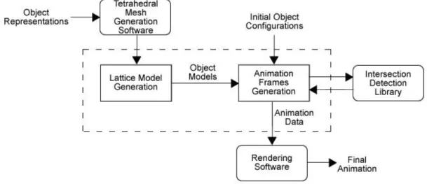
Creating a complete fracture animation is a multi step process. In our system, firstly, models are created for describing each object in the animation scene. The objects are initially represented by their polygonal surface descriptions. For the fracture process, a tetrahedral mesh and finally a lattice model of each object is constructed. After creation of these models, the animation steps are calculated according to the specified initial configurations of the objects. Finally, the cal-culated animation is rendered frame by frame, creating the final output of the program. Figure 1.1 gives a more detailed graphical overview of the animation generation process:

Figure 1.1: Overview of the animation generation process

1.2

Organization of the Thesis

The organization of this thesis is as follows: Chapter 2 provides a detailed re-view of the existing fracture and related deformation techniques in the literature. Chapter 3 explores the object model proposed by Smith, Witkin, and Baraff [23] that forms the basis for the simulation of the fracturing process we use. The process of generating each animation frame, which combines the rigid body and

CHAPTER 1. INTRODUCTION 4

the fracture simulation techniques, are described in Chapter 4. Chapter 5 provide the details of the dust formation feature of the system. Visual and numerical re-sults of the system along with implementation details and a comparison between the optimized and the unoptimised system are provided in Chapter 6. Finally, Chapter 7 provides conclusions and suggestions for future work.

In the appendices A and B, you can find the contact calculation derivations skipped in the main text for the sake of clearness. Also detailed information on how the system works is presented in Appendix C.

Chapter 2

Background

In computer graphics community, modeling deformations has a long history. Since fracture process can be considered a deformation, many methods later used for the animation of brittle fracture is adapted from deformation studies. Hence, in this section we will also examine some techniques developed for modeling deformations that act as a base for fracture studies, rather than just focusing on the area of brittle fracture.

The fracture process is hard to simulate using non-physical methods such as key framing or by methods that use purely geometric approaches to model deformation where bodies are deformed by modifying some control points or shape parameters [8]. Even though the computations are very fast in such methods, since the system has no information about the manipulated bodies, the final animations depend mostly on the animator’s expertise. As the objects get more complex, it becomes extremely hard to model the behavior.

In literature, there are very efficient non-physical methods that produce accu-rate results for generating crack patterns. These mainly map crack patterns to a surface or a volume (see [5, 10]). However, such methods are mainly used for gen-erating crack patterns in solo images rather than running animations. Because voxelization or tetrahedralization of the objects is not necessary, these methods are not limited in resolution. Small or very thin crack patterns can be generated,

CHAPTER 2. BACKGROUND 6

yet again, this process depends on the animator’s talents.

Physically-based simulation is utilized in computer graphics for many applica-tions. In the late eighties, Terzopoulos and Witkin introduced a hybrid model that represented a rigid body by its rigid and deformable components [27]. The rigid component handles the rigid-body motion while the elastic behavior is present only in the deformable displacement component. This approach aims solving the ill-conditioning of the discrete motion equations as the rigidity of the ob-ject increases. The computational cost, on the other hand, does not significantly improve as intended with this method.

Again, Terzopoulos and Fleischer generalized this work to encompass vis-coelasticity, plasticity, and fracture in deformable bodies [26, 25]. They used forces that depend on the velocities of mesh points and spatial partial derivatives of the displacement function. Fracture is realized by breaking connections in the mesh. Although this work is not directly focused on fracture, the technique could be applied to animations such as tearing paper.

In 1991, Norton et al. [13] used a mass-spring system specifically for modeling fracture. In this model, the objects were subdivided into a set of equal sized cubes connected with springs. This elastic network proved to be cumbersome in case of the existence of large objects.

Later, in 1999, O’Brien and Hodgins [15] presented a work for crack initial-ization and propagation. Their method uses stress and strain tensors computed over a Finite Element Method (FEM) to determine the place where the cracks will initialize and in which direction they will propagate. Also they used a local re-meshing algorithm to correctly preserve the direction of the fracture by split-ting the elements along the fracture boundaries to provide more realistic results. Later the techniques in this study are extended to handle ductile fracture as well [16, 14]. The results achieved by applying these techniques are strikingly good but the used continuum mechanics techniques are computationally demanding.

In 2000, Smith, Witkin, and Baraff [23, 24] came up with a method that uses a system of point-masses connected by workless, distance preserving constraints

CHAPTER 2. BACKGROUND 7

to model the object. The forces exerted by the rigid constraints are calculated using Lagrange multipliers. The simulation is realized as a result of solving a large, sparse, linear system using the conjugate gradient method. The method presents a much faster solution than that of O’Brien et al. with still realistic outputs.

In 2001 M¨uller et al. [12] came up with the idea of using a hybrid approach similar to that of Terzopoulos et al. [27] for realizing deformations and fracture in real time. The difference is that their method is hybrid in time. The dis-placements, stresses and fracture bases are computed on a continuous model only at collision events. They use the FEM as O’Brien et al. [15] do. However, they accelerate the core procedures of the FEM to work in near real time. The method uses the internal principal stress components provided by the FEM computation to determine fracture locations and orientations. In 2004, M¨uller et al. [11] ex-tends the existing model to handle elastic and plastic deformations as well. Also, in this study, a method to animate fracture with a high resolution tetrahedral mesh is introduced. An object is represented by a low resolution volumetric mesh for the FEM simulation, and a high resolution surface mesh for rendering. The low resolution mesh provides enough information for accurate results whereas the high resolution surface mesh allows rendering to be done in the desired quality without loss of performance.

In 2005, Pauly et al. [17] proposed a different technique for simulating frac-ture. Their method, as opposed to the other techniques, does not work on a mesh for fracturing elastic and plastic materials. Instead, they use a highly dynamic surface and volume sampling method which is supposed to solve stability prob-lems in mesh-based techniques. System uses advancing crack fronts and fracture surfaces within a volume, where a body is composed of simulation nodes. When a crack is formed, the nodal shape functions are adapted. Complex fracture patterns can be achieved by altering the crack fronts via a small set of topolog-ical operations for splitting, merging, and terminating. This way, they achieve continuous crack patterns with detailed fracture surfaces.

Chapter 3

Object Models

The objects we use in the system are initially represented via either polygonal surface or Constructive Solid Geometry (CSG) representations. However such representations are not adequate for performing fracture calculations on. We adopted Smith et al.’s lattice model [23].

For generating the lattice model, initial object models are tetrahedralized. Publicly available mesh generation software, NETGEN [21], is used for generat-ing the tetrahedral meshes. NETGEN is an open-source automatic mesh genera-tion tool for two and three dimensions. It comes as a stand-alone program with graphical user interface, and as a C++ library to be linked into another applica-tion. NETGEN accepts CSG and polygonal surface representations as input and creates their tetrahedral meshes. Also, applying a built-in uniform refinement algorithm can change the granularity of these meshes.

Once the tetrahedral mesh model is constructed, it is transformed into the final lattice representation. This representation is the Voronoi complement or dual of the solid object, which is basically a mesh of point masses -each representing a tetrahedron- connected to each other via workless distance-preserving constraints. Although it is similar to the simple spring-mass system, this model proves to be more advantageous for our purpose. Since we are dealing with brittle objects, the springs should be stiff enough to prevent visible plastic deformations in a

CHAPTER 3. OBJECT MODELS 9

Figure 3.1: A geometric object and its tetrahedral mesh, generated by NETGEN

spring-mass system. For a perfectly brittle object, the springs are infinitely stiff. In the lattice model we use rigid constraints instead of springs, hence rather than calculating displacements, we calculate the forces that the constraints produce in response to an applied impulse. The point masses represent the micro-fragments of the object, and the constraints represent the physical strength of the bond between these micro fragments. In case the force applied on a bond due to some impact exceeds a limit, the bond is broken, realizing the fracture effect.

However it is crucial to understand that these constraints are not force vectors themselves. In a real-world material, the intermolecular bonds hold the elements together such that the total force acting on an element is zero, serving to ensure equilibrium. In such a case the sum of the vectors holding an element is always zero. Hence, if these constraints were such vectors, removing or changing the value of one of these would eventually change the neighboring vectors’ values. In our case, the bonds only determine how close the material is to breaking at that specific point.

For generating the point masses and the constraints between them, the infor-mation from the tetrahedral meshes of the objects is used. For each tetrahedron in the mesh, a point mass is located at its center of gravity. The mass of each point is a function of the volume of the tetrahedron it represents, and the density of the material at that point. Also, for each pair of tetrahedra with a shared face, the corresponding point masses are connected with a rigid constraint, which has strength inversely proportional to the area of the shared face (Figure 3.2). By

CHAPTER 3. OBJECT MODELS 10

generating the lattice model in this manner, the geometry of an object becomes the effective factor in determining its breaking behavior.

Figure 3.2: Two tetrahedra and the corresponding lattice model. Adapted from [23]

Figure 3.3 displays the tetrahedral mesh and lattice of a simple object. The tetrahedral mesh is rendered in blue. The lattice as drawn in this figure consists of the connections within the model. In other words, the lines rendered in white are rigid constraints that connect the masses. Upon closer inspection, the reader can observe that each tetrahedron is connected with its neighbors via white lines.

Figure 3.3: The lattice and the tetrahedral mesh of an object rendered in white and blue respectively.

CHAPTER 3. OBJECT MODELS 11

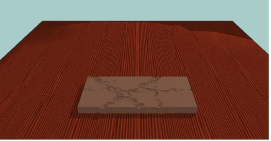
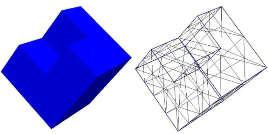
Some heuristics can also be applied after this step to achieve some user control and flexibility on the fracturing behavior of the objects. Cleaving planes are used for systematically reducing or increasing the connection strengths along a cross section of the objects. This way the user can define areas that are required to break or remain intact. Figure 3.4 illustrates the effect of cleaving on an object. The frame is generated by cleaving the rectangular block and letting it fall to the ground. The block is subjected to eight cleaving operations, where the regions between parallel planes are weakened and other regions are strengthened for a more dramatic result. When the block hits the ground, fracture takes place in the weak regions, which eventually make up a cross and a plus sign on the block. Three-dimensional noise and turbulence functions [18, 19] also provide a way to procedurally change the connection strength of the objects to achieve different fracturing behavior under the same initial conditions.

Chapter 4

Fracture Simulation

Our system is mainly a tool for manipulating objects in a 3D scene. It is a physics simulator in which objects can be subject to fracture. The fracture can be the result of a direct impact on the object as well as the indirect effect of an artificial force field. As mentioned earlier, the fracture calculations are only done at collision instants. The bodies act as unconstrained rigid bodies when there are no impacts. From now on, the notation used by Witkin et al. [30] will be used to denote derivatives, where a single dot is used for the first order time derivative and two dots denote second order time derivative.

The simulator works by generating an animation frame per time step. For generating the animation frames, the motion paths of the objects in the scene are calculated, and their updated positions and orientations are determined for each frame. In the case of a contact between two objects, the motion paths of the objects are updated and fracture calculations are performed. If these calculations result in the shattering of the object, the resulting shards are modeled as new objects and they are included in the animation calculations. This process is repeated until all the desired frames of animation are generated.

For updating the positions and orientations of the objects at each frame, a technique called bisection is applied. As it can clearly be seen from the pseudo-code description on the next page, this technique divides a single interval between

CHAPTER 4. FRACTURE SIMULATION 13

two frames into smaller sub-intervals, ensuring that the objects are in valid con-figurations at the end of each sub-interval.

Algorithm: Generating the Animation Frames

GENERATE FRAMES(numF rames, f rameDuration) 1 currentF rame ← 1

2 while currentF rame < numF rames 3 remainingDuration ← f rameDuration 4 updateDuration ← f rameDuration 5 while remainingDuration > 0

6 UPDATE OBJECTS(updateDuration) 7 if no objects intersect

8 remainingDuration ← remainingDuration − updateDuration 9 updateDuration ← remainingDuration

10 else updateDuration ← updateDuration/2

11 PROCESS CONTACTS

12 PROCESS FRACTURE

13 if dust creation is selected

14 create particle systems where necessary

Determining whether the objects are in valid configurations at the end of each sub-interval requires intersection tests between each pair of objects. For performing these tests, a publicly available software library, FreeSOLID [28], is used. After creating the object models, each object is also given to the library by describing their shapes and initial configurations. During the generation of the animation frames, the configuration changes of the objects are also reflected to FreeSOLID and the intersection tests are performed via the functionality provided by the library.

After getting a valid configuration, calculations are performed to handle the contacts between the objects as well as to determine the fracturing of the objects. In the remainder of this chapter, details of the motion, contact, and fracture

CHAPTER 4. FRACTURE SIMULATION 14

calculations are discussed. The derivations in sections 4.1 and 4.2 are based on the course notes prepared by Baraff [3].

4.1

Unconstrained Motion Calculations

Unconstrained motion means that the motion of the body is not restricted by any constraints so that any position in space is valid for the object. Although, obvi-ously this is not the case in real life and in fracture animation, these calculations form the basis of animation calculations since they handle all the situations that do not involve collisions.

We define the state of an object in space by its state vector X(t) as:

X(t) =         x(t) Q(t) P (t) L(t)         . (4.1)

Here, x(t) is a 3-vector that describes the position of the center of mass of the object, Q(t) is a quaternion that describes the orientation of the object around its center of mass, P (t) and L(t) are 3-vectors that respectively describe the linear and angular momentums of the object.

The linear momentum of an object P (t) is defined as:

P (t) = mv(t) . (4.2)

Hence, the linear velocity v(t) of an object is

v(t) = P (t)

CHAPTER 4. FRACTURE SIMULATION 15

Since x(t) is the position of the center of mass of the object, its time derivative is simply the linear velocity of the object.

˙x(t) = v(t) . (4.4)

Similarly, the angular momentum of an object L(t) is defined as:

L(t) = l(t)w(t) , (4.5)

where, l(t) is the rank-two inertia tensor for an object consisting of n point masses, each with mass mi, and position vector ri relative to the position of the center of

mass of the object:

l(t) = n X i=0      mi(riy0 2 + r0_iz2) −mir0ixr 0 iy −mir0ixr 0 iz −mir0ixr 0 iy mi(rix0 2 + r0_iz2) −mir0iyr 0 iz −mir0ixr 0 iz −miriy0 r 0 iz mi(r0ix 2 + r_iy0 2)      . (4.6)

Similar to the linear velocity case, the angular velocity of the object can be defined as:

w(t) = l−1(t)L(t) . (4.7)

If the angular velocity of an object is w(t), this means that the object is rotating about the axis w(t) with a velocity of magnitude |w(t)| . Thus, the orientation of the object after rotating with the angular velocity of w(t) for a period of time ∆t = t − t0 can be represented with the quaternion:

Q(t) = " cos |w(t)| ∆ t 2 ! , sin |w(t)| ∆ t w ! w(t) |w(t)| # Q(t0) . (4.8)

Taking t = t0 and differentiating with respect to time, we get the formula for

˙ Q(t):

CHAPTER 4. FRACTURE SIMULATION 16 ˙ Q(t) = " 0,w(t0) 2 # Q(t0) . (4.9)

The product [0, w(t)] Q(t) is abbreviated as w(t)Q(t), letting ˙Q(t) be

˙

Q(t) = 1

2w(t)Q(t) . (4.10)

The linear acceleration of the object can be described by taking the time derivative of equation 4.3:

˙v(t) = ˙ P (t)

m . (4.11)

Reorganizing and applying Newton’s second law of motion we get

˙

P (t) = m ˙v(t) = F (t) . (4.12)

Similarly, the time derivative of the angular momentum of the object can be defined by taking the time derivative of equation 4.5:

˙

L(t) = ˙l(t)w(t) + l(t) ˙w(t) = τ (t) , (4.13)

where τ (t) is the total torque acting on the object.

By combining equations 4.4, 4.9, 4.12 and 4.13, the time derivative of the state vector can be constructed as:

˙ X(t) =         v(t) 1 2w(t)Q(t) F (t) τ (t)         , (4.14)

CHAPTER 4. FRACTURE SIMULATION 17

where v(t) is the linear velocity of the object, F (t) is the total force acting on the object and τ (t) is the total torque acting on the object. The state of an object at time t is defined by the ordinary differential equation (ODE):

d

dtX(t) = ˙X(t) . (4.15)

For calculating the motion of an object, this ODE must be integrated for the duration of each animation frame. At the beginning of the animation, the initial values for four components of the state vector are given as the initial configuration of the object, and during the course of the animation the state vector is updated at each motion calculation. This way, the motion calculation becomes an initial value problem from which the value of X(t) can be computed for any value of t. An ODE integrator using the Fourth-Order Runge-Kutta method with adaptive step sizing is implemented to solve this initial value problem and calculate the motion of the objects (see [20]). By applying an adaptive step sizing algorithm, an upper bound for error is maintained in motion calculations.

4.2

Contact Calculations

So far, the motion calculations are performed with the assumption that the move-ment of the object is unconstrained. However this assumption is not valid when two objects come into contact with each other since motion of real world objects is constrained with impenetrability constraints. In other words, in real world no two objects can have overlapping volumes. Thus, in order to be able to realistically simulate the motion of the objects in the animation scene, the impenetrability constraints must be enforced [2].

A constraint can be defined by a function which takes certain values when it is satisfied. The impenetrability constraints can be defined as inequality constraints such that for the constraint function C((x(t)) , we should have:

CHAPTER 4. FRACTURE SIMULATION 18

C(x(t)) ≥ 0 , (4.16)

for all valid positions x(t) of the object.

Whenever the impenetrability constraints are satisfied, we consider the motion of the object unconstrained and perform the calculations described in the previous section to determine it. In case an impenetrability constraint is unsatisfied, the last point in time when the constraint was satisfied is found using the bisection technique described earlier, and necessary actions are taken in order to make the object satisfy the constraints in the future.

If the impenetrability constraint for a pair of objects is not satisfied at a given time t, this means that these objects have overlapping volumes, i.e. they are intersecting. In such a case the last point in time when the constraint was satisfied is the time when the objects were in contact. So, by applying appropriate response on the objects when they are in contact, the impenetrability constraints can be enforced throughout the animation.

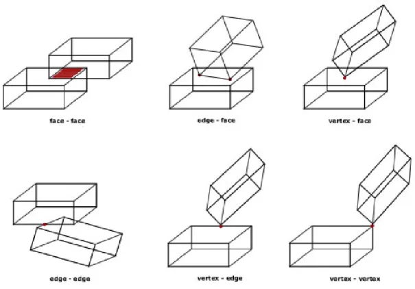
A contact between two objects is defined by a contact normal and a contact point extracted from contacting features of the two objects. In the case of multiple contact points between objects, each contact point is considered as a separate contact. In terms of contacting features, contacts can be categorized into six groups (see Figure 4.1). Two of these contact types, edge and vertex-vertex, are considered degenerate in the sense that a contact normal cannot be determined for them. Since the probability of a degenerate contact occurring between two objects is very low, they are discarded while handling the contacts [1]. For the remaining four contact types the contact points and the corresponding contact normals are determined as follows:

• Face-Face: The contact normal is the surface normal of one of the con-tacting faces. The contact points are the vertices of the polygon that define the intersection of the faces.

CHAPTER 4. FRACTURE SIMULATION 19

Figure 4.1: Six types of contacts according to the contacting features. In each condition contact points are marked red.

face. The contact points are the two endpoints of the edge segment that intersect with the face.

• Vertex-Face: The contact normal is the surface normal of the face. The only contact point is the contacting vertex.

• Edge-Edge: In this case it is assumed that the contacting edges are not collinear. So, the contact normal is the normal of the plane defined by the lines that go through the two contacting edges. The only contact point is the intersection point of the two edges.

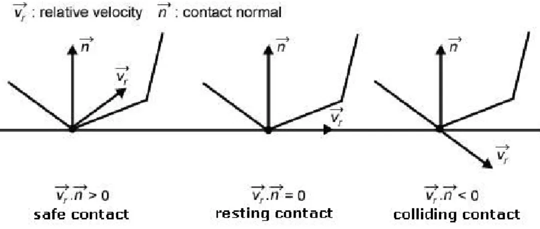
After the contact points and the corresponding contact normals of a contact are determined, the appropriate response for the contact is determined by looking at the projection of the relative velocity of the objects at the contact points over the contact normal. Figure 4.2 shows the three possible cases which are handled

CHAPTER 4. FRACTURE SIMULATION 20

differently.

Figure 4.2: Three types of contacts according to the relative velocities

If the projected relative velocity is greater than zero, it means that the contact-ing objects are actually separatcontact-ing from each other, thus no response is necessary to enforce the impenetrability constraint. If the projected relative velocity is zero, it means that the contacting objects are moving together. This type of contact is called a resting contact and it is handled by calculating contact forces that act on the objects at the contact points. If the projected relative velocity is less than zero, it means that the contacting points are moving towards each other. This type of contact is called a colliding contact and it is handled by calculating con-tact impulses that act on the objects at the concon-tact points. In the following two subsections the details of the colliding contact and resting contact calculations will be discussed.

4.2.1

Colliding Contact Calculations

Colliding contact is the type of contact at which the contacting objects are moving towards each other. Mathematically, the quantity vrel can be defined as:

vrel = ˆn(tc) · ( ˙pa(tc) − ˙pb(tc)) , (4.17)

where, ˙pa(t) and ˙pb(t) are respectively the velocities of the contact points on the

CHAPTER 4. FRACTURE SIMULATION 21

time of the contact. The quantity vrel gives the component of the relative velocity

˙

pa(tc) − ˙pb(tc) in the ˆn(tc) direction. In case vrel is positive, the bodies are safely

moving away from each other. If vrel is negative then we have a colliding contact.

vrel being zero implies that the bodies are resting on each other and this case is

explained in the next section.

In real life an elastic collision is a process in which the colliding objects remain in contact for some duration of time. During this duration contact forces, which are equal in magnitude and reverse in direction, act on the objects. However, since all the objects in the animation scene are brittle objects, the collisions can safely be reduced to instantaneous events without reducing the quality of the resulting animation. By reducing the contact duration to an instance, it is also necessary to reduce the effect of the contact forces over the duration of the collision to a single instance. The vector I, which is the impulse that acts on objects that are in contact can be defined as:

I =

Z

F (t)dt , (4.18)

where, F (t) is the vector function that defines the contact force acting on the object during the course of the contact. The required change in the velocity of the object due to this collision can be achieved by applying the changes ∆P (t) and ∆L(t) to the linear and angular momentums of the object respectively:

∆P (tc) = I (4.19)

∆L(tc) = (p − x(tc)) × I . (4.20)

Here, p is the contact point, x(t) is the position of the center of mass of the object at time t, and tc is the time of the collision. Detailed derivations of these

formulas, and details on how to calculate the impulse vector I can be found in Appendix A.

CHAPTER 4. FRACTURE SIMULATION 22

4.2.2

Resting Contact Calculations

In the case of the resting contacts the contacting objects are neither moving towards nor apart from each other at the contact point. However the impenetra-bility constraints can still be violated if the contacting objects are accelerating towards each other. In this case contact forces must be calculated and applied on the objects in order to prevent them from accelerating into each other.

The time derivative of vrel, which is the projection of the relative acceleration

of the objects over the contact normal at the contact point, can be defined as:

˙vrel = arel = ˆn(tc) · ( ¨pa(tc) − ¨pb(tc)) + 2 ˙ˆn(tc) · ( ˙pa(tc) − ˙pb(tc)) , (4.21)

where ¨pa(t) and ¨pb(t) are the accelerations and ˙pa(t) and ˙pb(t) are the velocities

of the contact points on the contacting objects, ˆn(t) is the unit contact normal vector and tc is the time of contact.

Besides requiring arelto be nonnegative, two other conditions must be satisfied

while calculating the contact forces. Firstly, the contact forces should never be attractive. Secondly, the contact forces must remain as long as the corresponding contact remains and no more. By combining these conditions together, we can formulate the problem of finding the contact forces as a quadratic programming (QP) problem as follows:

min fT(Af + b) subject to

 



(Af + b) ≥ 0

f ≥ 0 . (4.22)

Here (Af + b) is the concatenation of all the arel values for all of the resting

contacts and f is the concatenated vector of contact forces that are required for enforcing the impenetrability constraints. The concatenated vector is separated into its force dependent and force independent parts in order to be able to for-mulate it as a QP problem. The details of formulating the QP problem can be found in Appendix B.

CHAPTER 4. FRACTURE SIMULATION 23

After the QP problem is formulated, it is given to the OOQP library [6, 7], a publicly available QP problem solver, and the resulting contact forces are applied to the objects.

4.3

Fracture Calculations

As mentioned earlier, our system uses two different techniques for realizing frac-ture. In both techniques the simulation of the fracturing process makes use of the lattice model representation of the objects. The crack initialization is invoked due to some external force applied to a point on the outer surface or in the inner region of the object. Obviously, the forces can be either artificial, explicitly de-fined to initiate a fracture, or impulses due to colliding contacts, calculated while enforcing the impenetrability constraints. Upon the application of such a force, in response, constraint forces are calculated and the constraints are modified ac-cordingly. What differs in the two approaches implemented for this thesis is how we modify the connection strengths in the lattice model. Yet, regardless of how the modification is done, we enforce the distance-preserving constraints on the lattice of particles. In case the constraint force for a connection is greater than the current constraint strength, that constraint is removed. Otherwise the existing connection strength is weakened by the amount of the constraint force applied on it. Any constraint for which the resulting connection strength is weaker than a predefined constraint force threshold is removed.

In the next two sections, we will examine two different algorithms used for animating the fracture effects. The first algorithm explained in Section 4.3.1 is proposed by Smith et al. [23, 24]. This algorithm computes fracture as a local event, determining the force acting on the tetrahedra using Lagrange multipliers. Whenever there is an impact on the body such forces are computed and bonds are broken to initiate fracture. Applying the forces in a stepwise manner helps obtaining crack propagation. However no global information is valid for material properties. Hence the cracks seem to occur at collision regions only. Also it is very hard to simulate different materials with this algorithm. The terms first algorithm

CHAPTER 4. FRACTURE SIMULATION 24

and slow algorithm will be interchangeably used for citing this algorithm.

The second algorithm explained in Section 4.3.2 is proposed by O’Brien et al. [15], and then optimized by M¨uller et al. [12] to run in near-real-time. This method makes use of stress tensors within an object when calculating the fracture. In fact, at each tetrahedra of the model stress is hidden. Upon an impulse this stress is exposed and in our case this stress is expressed as fracture. This formulation assumes the fracture will start at the tetrahedra where the stress is maximum. When such a tetrahedra is found, a collision plane is constructed to form the cracks. This algorithm represents the body globally. It is expected to see large cracks where the body is prone to failing, instead of having all cracks near the impact region. The terms second algorithm and fast algorithm will be interchangeably used when talking about this algorithm.

4.3.1

Slow Fracture Simulation

For calculating the constraint forces that act on the system of particles of the object, the positions of the particles are placed in a vector named q, such that, for an n particle system, q is a 3n × 1 vector defined as:

q =      q1 .. . qn      . (4.23)

A mass matrix M is defined in such a way that it holds the particles’ masses on the main diagonal, and 0’s elsewhere. So a mass matrix for n particles in 3D is a 3n × 3n matrix with diagonal elements {m1, m1, m1, m2, m2, m2, ..., mn, mn, mn}.

Finally, a global force vector F is obtained by joining the forces on all particles, just as we did for the positions. From Newton’s Second Law of Motion, the global equation on the particle system is as follows:

¨

CHAPTER 4. FRACTURE SIMULATION 25

where M−1 is the inverse of the mass matrix, M .

A similar global notation will be used for the set of constraints: Concatenating all scalar constraint functions form the vector function C(q). In 3D, for n particles subject to m constraints, this constraint function has an input of a 3n × 1 vector, and an output of an m × 1 vector. In our case, this constraint function consists of the scalar distance-preserving constraints in the form:

Ci(pa, pb) = kpa− pbk − di , (4.25)

where pa and pb are the positions of two particles connected to constraint i, and

di is the distance between the particles that needs to be preserved.

Assuming initial positions and velocities are legal, we try to come up with a feasible constraint force vector ˆF such that the distance preserving constraints are held. In other words, for the initial conditions that satisfy C(q) = ˙C(q) = 0, we are trying to find the constraint force vector ˆF , such that, when added to F , guarantees ¨C(q) = 0. In order not to break the balance of the system, it has to be assured that no work is done by the constraint forces in system, for all valid position vectors:

ˆ

F . ˙q = 0 ∀ ˙q . (4.26)

All vectors that satisfy this requirement can be written as

ˆ

F = JTλ , (4.27)

where J is the Jacobian of C, and is equal to ∂C_∂q. Here, λ is a vector with the same dimensions as C. The components of λ are known as Lagrange multipliers and they tell how much of each constraint gradient is mixed into the constraint force. From 4.27:

J M−1JTλ = −J M−1F . (4.28)

Note that the above formula is a system of linear equations of the form Ax = b where A is a matrix and x and b are vectors. By calculating the λ vector from equation 4.28 and placing it in equation 4.27, the constraint force vector ˆF , which satisfies the given rigidity constraints can be calculated. To ensure that the λ

CHAPTER 4. FRACTURE SIMULATION 26

vector is a physically realizable solution for the system, the conjugate gradient method [22], which gives the minimum norm solution of the system, is used since the minimum norm solution of the system is also the physically realizable one.

Even though the constraint force vector ˆF could be found in a single step, it produces better results to do it in multiple steps, transmitting forces among the particles at each step before they are removed, given that they transmit no more force than the breaking stress would tolerate. Thus, each ˆF is used as an input to the next iteration.

Solving the problem in multiple steps, the impact force is increased gradually at each step. This way, as opposed to creating a single impulse, a more realistic impulse history is created.

4.3.1.1 Modifying the Connection Strengths

Once a crack is invoked at some point of the model, due to some external or internal force, the connection strengths are modified procedurally. In real world, when a brittle object is breaking, the energy required for starting a new crack is much higher than propagating an already existing crack. Thus, to imitate this behavior, while removing a newly broken constraint, the neighboring constraints, which are adjacent to the faces of the newly broken constraint, are weakened. This way, the relative probability of growing of an existing crack to the initiation of a new one is increased.

Obviously, the connections that are close to the crack region will be affected more than the connections that are far away from it. The strengths are modi-fied gradually. However, weakening the connection strengths uniformly produces cracks that are visually artificial. Hence, in order to introduce a randomness into the crack pattern, some connections are made weaker than the others. These connections, and the amount of weakening are selected randomly. This opera-tion introduces no performance loss, yet it is very successful in generating crack patterns. Moreover, even though two geometrically same objects are broken un-der the same conditions, the system produces distinct final crack patterns and

CHAPTER 4. FRACTURE SIMULATION 27

formation of longer cracks is achieved.

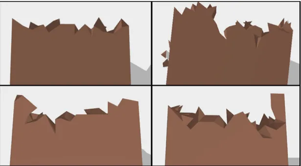
Fig. 4.3 compares the effect of modifying the connections with and without the given technique. The object in upper left image is broken with the original algorithm, while the objects shown in the other three images are broken with our modified one. It is easily observable how the crack patterns change every time the algorithm is run. In addition, with the technique used here, not only a successful randomization in cracks is achieved, but also the cracks formed after the fracture are longer.

Figure 4.3: A comparison of the crack patterns generated by modifying the con-nection strengths uniformly (upper left image) and with the given algorithm (other images).

4.3.2

Fast Fracture Simulation

Our near-real-time solution makes use of the stress supported by a body when handling fracture as proposed by O’Brien et al. [15] and then improved by M¨uller et al. [12] with slight modifications.

Stress is a measure of force acting on per unit area within a body. Cauchy’s principle states that, within a material the forces imposed by a closed volume are

CHAPTER 4. FRACTURE SIMULATION 28

in equilibrium with the forces imposed on the closed volume by the remainder of the body [29]. Hence we are trying to find a set of forces imposed on each tetrahedra in response to a force acting on the body.

The stress at a point can be found by considering a small element of the body with area ∆A, perpendicular to which a force ∆F is applied. By making the element infinitely small, the scalar stress σ can be found:

σ = lim ∆ A→0 ∆ F ∆ A = dF dA . (4.29)

Stress can be described by a second-order tensor since the behavior of the body is independent of the coordinate systems the body is located on. In 3D, the internal force acting on area ∆A of a plane can be partitioned into three components: one normal to the plane and two parallel to the plane. Divided by ∆A, the normal component gives the normal stress, denoted by σ; and the parallel components give the shear stresses, denoted by τ . The Cauchy stress tensor is a 3 × 3 matrix. σ =      σx τxy τxz τyx σy τyz τzx τzy σz      . (4.30)

Here, σi, i ∈ {x, y, z} denotes the normal stress and τij, with i, j ∈ {x, y, z}

and i 6= j, values are shear stresses as mentioned earlier. In case of equilibrium τxy = τyx, τxz = τzx, and τyz = τzy. Hence the tensor is also symmetric. This

matrix has 3 real eigenvalues, which denote the principal stresses. The related eigenvectors denote the principal stress directions. A positive eigenvalue stands for tensile stress while a negative one indicates compressive stress.

What M¨uller et al. [12] do for determining the breaking behavior object is to perform an eigenvalue decomposition for each tetrahedron in the object model. This way, they compute the stress at each atomic unit of the material. Let λmax be the largest eigenvalue calculated for the whole body. If λmax is greater

CHAPTER 4. FRACTURE SIMULATION 29

than a given threshold, fracture takes place. The tetrahedron with the greatest eigenvalue is where the crack initialization will begin. This is a realistic approach since in real world fracture is initiated to release the greatest energy in response to an external/internal effect.

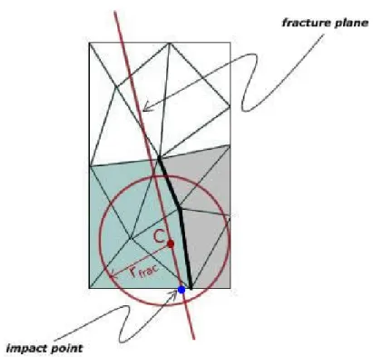
A fracture plane perpendicular to the eigenvector of λmax is obtained upon an

impact. and within a radius rf rac, tetrahedra are split if their center of masses

fall on opposite sides of the fracture plane (see Figure 4.4). rf rac is determined

according to the material properties and the stress magnitude.

Only the tetrahedra within a radius rf rac from the tetrahedron under

ten-sile stress -the one with the largest eigenvalue- are examined. The constraint strengths between neighboring tetrahedra, the center of masses of which fall on opposite sides of the fracture plane are updated according to the stress acting on them.

Our approach differs slightly from this approach, not by methodology, but by the number of affected tetrahedra and the calculation of the stress tensor. We, instead of calculating the eigenvalues of all tetrahedra, do a localized analysis. Our system works on the assumption that the largest stress will be close to the impact point. Experiments showed that instead of calculating the eigenvalues for all tetrahedra, only considering the ones close enough to the impact point proves to give satisfying results. In fact, in most cases, these tetrahedra are most prone to stress within a body. This way, we radically decrease the number of computations.

Also for the stress tensor we do a simplified calculation. We ignore the effects of the shear stresses, this way, the eigenvalues are equal to the normal stress values, while unit vectors are the eigenvectors. For the diagonal elements σi’s,

we use the x, y, z components of an effective force fef f acting on a tetrahedron.

Firstly the average of all contacts that are fairly close to each other are used to form the vector favg. The closeness is determined by thresholding the distance

CHAPTER 4. FRACTURE SIMULATION 30

Figure 4.4: Effect of the fracture plane and radius rf rac on crack generation.

Adapted from [12]

fef f = (favg/(ra)2)vola) , (4.31)

where ra is the distance between tetrahedron a’s center of mass and fef f’s

appli-cation point; and vola is the volume of the corresponding tetrahedron a. For a

tetrahedron with vertex positions p1, p2, p3, and p4, the volume is

vol = 1

6[(p2− p1) × (p3− p1)] · (p4 − p1) . (4.32) Another modification to M¨uller’s method is done when modifying the re-lated connection strengths. M¨uller removes all connections within a given radius through the fracture plane if the largest eigenvalue exceeds a given limit. However, we chose to modify the connection strengths within the boundary by the relative stress acting between two tetrahedra. Changing the connection strengths, again, is done as a multi-step process to enhance the reality of the resulting animations.

CHAPTER 4. FRACTURE SIMULATION 31

4.4

Rendering

The last step of animation generation process is rendering the animation scenes frame by frame, which creates a realistic looking output. After calculating each frame of the animation, the program outputs a file that the rendering software can read and render, which includes only the object data on scene. By changing the global effects, such as lighting, camera, etc, several animations can be prepared for a single fracture.

Persistence of Vision Raytracer (POV-Ray) software v.3.6 [4] is used for real-izing this step. The software has a scripting language, namely POV-Ray 3 Scene Description Language, which allows an easy way to describe a scene in plain ASCII text format. The language, similar to many widely used programming languages, consists of identifiers, reserved keywords, floating-point expressions, strings, special symbols, and comments. It also includes predefined structures for several shapes, such as spheres, planes etc. In addition there are methods for modifying the camera location and angle and for illuminating the scene. POV-Ray allows applying texture mapping or photon mapping to the objects; adding interiors to them, i.e. to give a feeling of glass and adding atmospheric effects such as fog, to the scene. In addition, the light sources, which vary from point light sources to spotlights, can be used extensively, where a scene can contain multiple light sources.

Since the objects in the implemented solution are described as tetrahedral meshes, the Mesh2 object of POV-Ray, which is a representation of a mesh, is used. A Mesh2 object is given the coordinates of each vertex, and information on which vertices will create triangles in the tetrahedral mesh. Optionally, normal vectors on each vertex can be calculated by interpolating the face normals, and given to the Mesh2 object, to eliminate sharp corners and give a smoother look to the object. POV-Ray generates bitmap files that contain the rendered scene for each frame of the animation. These bitmap files are then put together to create a movie of the animation, by using a movie editor software.

Chapter 5

Dust Formation

We implemented a simple addition to the system to support dust formation upon impacts. This way, we achieve better visual results when many small fragments are created as a result of breaking clay-like materials. The dust effect also offers favorable results when the scene contains objects falling on earth.

Dust formation is a process independent of the algorithm used for generating the fracture effects. If the user chooses to create dust for the animation, regardless of the practiced algorithm, particle systems are created in case there is fracture. Each breaking object holds its own list of particle systems and is responsible for updating them. The number of generated particle systems depends on the number of impacts that trigger the fracture process. The particles are moved by basic particle dynamics, whereas the forces acting on the particles are calculated as a result of the impacts. Figure 5.1 presents selected frames from an animation in which dust is embedded. In the rest of this chapter, you can find the details of the particle system we use.

CHAPTER 5. DUST FORMATION 33

CHAPTER 5. DUST FORMATION 34

5.1

The Particle System

A particle system is basically a collection of points in space. These points, a.k.a. particles, go through a life cycle: they are born, change over time and finally die. Our particle system consists of particles and an emitter, which is responsible for creating the particles. Each particle in the system has position, velocity, and mass at a given time; it responds to forces and rests in the system for only a finite amount of time. Particles’ behavior is controlled by a stochastic process. When a particle comes to the end of its period in the system, it is taken into a pool, from where newly added particles are taken randomly. The particle system we use is implemented as explained by Lander [9].

Witkin provides an excellent explanation of particle dynamics in [31]. The particle motion is governed by Newton’s second law of motion:

F = ma . (5.1)

This equation can be represented in the form of two equations,

˙v = F/m , (5.2)

˙x = v . (5.3)

Clearly, for a given particle, F denotes the sum of forces acting on it, m is the mass, a is the acceleration, v is the velocity, and x is the position. Positions of the particles are updated at each animation frame by solving these two first order ODEs simultaneously.

The position and velocity, x and v, can be concatenated to form a 6-vector, called the phase space [31]. The phase space equation of motion is

CHAPTER 5. DUST FORMATION 35

A system of n particles is described by n copies of this equation, forming a 6n-vector.

The second main element of the particle system is the emitter. The emitter is responsible for generating new particles at a given rate as long as the total particle count does not exceed a threshold. The particles are generated at random positions in a bounding volume. Additionally, the emitter can assign varying initial velocities to the particles for randomization effects.

The forces acting on each particle is calculated by a different module. These forces can be due to both force fields and forces caused by collisions between objects within the environment. The force fields can be constant force fields, such as gravity; time dependent force fields, such as wind or turbulence; and velocity dependent force fields, such as drag. Each particle in the system is represented by a structure containing its position, velocity (which alone make up the phase space), force, and mass. An Euler ODE solver is used to determine the motion.

Given a time step, an Euler solver takes the derivatives in equations 5.2 and 5.3, scales the derivative vectors with the time step, adds the current state vector of the particle with the newly calculated values, and finally iterates the particle system’s clock.

In the implemented solution, particle systems are created at impact points whenever the corresponding impact magnitudes are over a threshold. An alter-native solution to reduce the number of particle systems would be by grouping nearby impacts together and creating a single particle system for the whole group. The impact magnitude also affects the particle system’s behavior. As the impact magnitude gets bigger, the total number of particles hosted by the particle system increases, resulting with a denser dust formation. Also the global force acting on the particle system is a function of the linear momentum of the object and the impact magnitude. This way, the harder the object hits another, the farther the particles are scattered.

The particles in our animations stay in the system for a very short time for visual accuracy. Hence we omitted calculations for collision detection and

CHAPTER 5. DUST FORMATION 36

response. Since the particles in the system are large in number, it is infeasible to consider them as being scene objects. Normally, the particles are thought of as points and simple point-to-plane collision detection and response actions can be taken.

5.2

Rendering

Particles in the system are represented as spheres. Each sphere is assigned a media, which uses spherical mapping, where a color mapping is used to color the dust. The color map is a function, which accepts the distance to the center of the sphere as an input. Also a turbulence function is applied on the dust media. Without the turbulence, the view would be duller with every particle having the same color map.

Chapter 6

Experimental Results

6.1

Visual Results

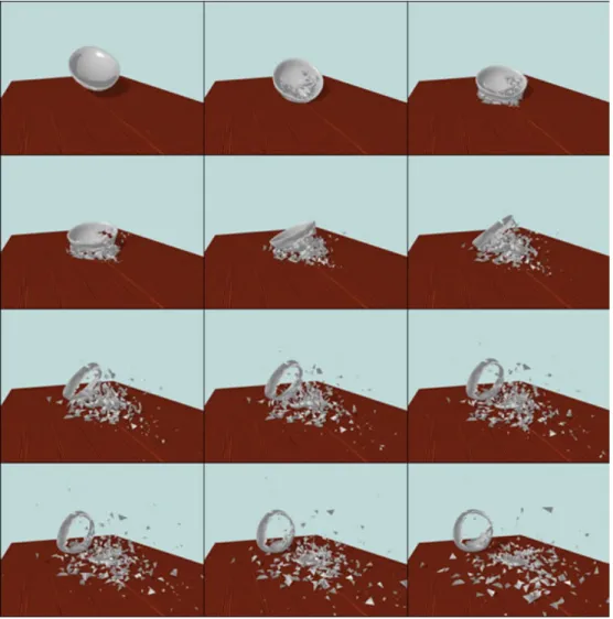
Figure 6.1 illustrates selected frames from an animation generated by the slow algorithm. The scene contains two objects: a breakable ceramic bowl and the floor. The sequence is generated by dropping the bowl from an altitude. Hitting the floor, the model is broken into pieces. As it can be seen from the figures, the process generates many interlocking fragments, which obey the dynamics rules. The bowl model consists of 4514 tetrahedra. After the fracture, the parts of the bowl that are far away from the contact point remain intact. As explained in Chapter 4, this is a natural outcome of the first algorithm: the fracture is initiated at the crack region and it can propagate only in a local area.

Figure 6.2 shows a scene where a ball falls onto a glass table. The scene is created using the fast algorithm. The table consists of two rectangular legs and a glass surface sitting on the legs. The legs are fixed objects that are only supportive parts and are omitted during the fracture calculations. The only breakable object, table surface consists of 3581 tetrahedra. The animation is constructed by locating an unbreakable ball on top of the table, and assigning a linear momentum pointing downwards to that ball. As a result of that linear momentum, the ball falls onto the glass table. The impact at the collision is great

CHAPTER 6. EXPERIMENTAL RESULTS 38

Figure 6.1: Ceramic bowl breaking upon falling to the ground (Animation gen-erated by the slow algorithm)

CHAPTER 6. EXPERIMENTAL RESULTS 39

Figure 6.2: Glass table breaking under the impact of a heavy ball (Animation generated by the fast algorithm)

enough to initiate fracture. The fracture is propagated through planes and the body is fragmented into mainly six large pieces. Besides, numerous fragments are created, which begin to move naturally within the simulation scene. As a result of the changing geometry, the bigger fragments, which are still fragile, slide towards the floor. Yet they do not shatter as a result of the collision with the floor. This implies that the secondary collision does not arouse an impact strong enough to initiate fracture.

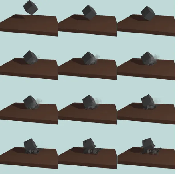
Figures 6.3 and 6.4 illustrate a visual comparison between the outputs of two algorithms. Both animations are created with exactly the same initial settings. The broken cube consists of 227 tetrahedra. In this comparison, the result of the second algorithm seem satisfying, even more realistic than that of the first algorithm. Note that in the output of the first algorithm (in Figure 6.3), we see a crack pattern only located near the impact region. This is expected since as we explained, the method uses a localized analysis when calculating the exerted forces on the bonds.

CHAPTER 6. EXPERIMENTAL RESULTS 40

The output of the second algorithm (in Figure 6.4), on the other hand provides a more diverse crack pattern. This pattern implies that the cube in our example was weaker at the diagonal. The tetrahedral meshes that NETGEN creates tend to be denser in the inner regions than they are at edges. As an assumption, we can say that as the tetrahedra get bigger, the strength of the bonds gets weaker. Hence, we have a physically convincing result.

However, the second algorithm sometimes produces undesired results. In Fig-ures 6.5 and 6.6, we see the resulting animation of the same scene, created with different algorithms. In this scene, the wall consists of 4080 tetrahedra. Again, in Figure 6.5 we see that the first algorithm only affects a small area on the wall. This is appropriate for a clay wall as rendered in the scene.

Figure 6.6 displays the output of the second algorithm. As mentioned ear-lier, this algorithm is dependent on the body properties of the object. Also since collision planes are used, the calculation of the collision radius is crucial. This calculation determines the crack growth range. Here in Figure 6.6, we see what happens when the collision radius is not selected properly. Such a distribution does not seem appropriate for a clay wall, but it would look better if the medium were glass. This implies that the second algorithm depends on some parame-ters which should be carefully selected by the animator. Selecting the radius differently, the animator might simulate a variety of different materials.

6.2

Performance Analysis

As discussed in Chapter 4, three major steps take place during the creation of an animation:

The first step, generation of the object models, is performed once for an animation scene, and the results are stored in a file. Also this is a very fast process, taking only a few seconds even for very large numbers of tetrahedra.

CHAPTER 6. EXPERIMENTAL RESULTS 41

CHAPTER 6. EXPERIMENTAL RESULTS 42

CHAPTER 6. EXPERIMENTAL RESULTS 43

CHAPTER 6. EXPERIMENTAL RESULTS 44

CHAPTER 6. EXPERIMENTAL RESULTS 45

As seen in Figure 6.7, the generation of the frames that are created just as the shattering occurs takes significantly more time than the remaining frames do. This bottleneck is solved significantly by the second algorithm. Note that even though this step remains to be very slow when compared with the rest of the simulation, there is no longer a huge gap between the processing times between frames.

Figure 6.7: Calculation times for the breaking cube animation (a) Fast Algorithm (b) Slow Algorithm (c) A close-up of the chart for both algorithms

In Table 6.1 the system’s performance comparison between two methods is illustrated. The performance is considered as being the duration of the most time consuming step in the animation: the fracture calculations. In both cases, the performance is measured with respect to the number of contacts that initiate fracture and the number of tetrahedra that make up the broken body. It is obvious

CHAPTER 6. EXPERIMENTAL RESULTS 46

that as the contact count increases, the gain achieved by the second algorithm is significant even though the system cannot work in real-time. Also a comparison is provided for cases where the user selects initiating the dust creation process or not. Obviously, the number of contacts affects the dust creation performance. The process gets slower when the contacts are high in number, since more particle systems are created in such a case, and motion calculations are performed for each particle system. ] of con tacts ] of tetra hedra

Performance (in msec)

Fast Slow

w dust w/o dust w dust w/o dust

4 227 32 16 1235 1203 13 227 125 47 2265 2219 88 227 344 310 3031 2719 129 4080 812 329 128375 123937 220 4080 1625 531 246922 237063 967 4080 6688 1671 555250 472078

Table 6.1: Computation time of the fracture calculations versus impulse and tetrahedra counts for both algorithms

The time required for the third step, visualization of the results, depends on many parameters. Naturally the number of objects within a scene along with the material properties and complexity of these objects directly affect rendering performance. Scenes that contain materials prone to internal reflections, such as glass, take more time to render. The number of light sources can be a minor factor in case the orientation of the light source lets us perceive otherwise not apparent details of some objects. Experiments show that rendering dust affects the performance unfavorably.