Simulation of a holographic 3-D television display

Λ'к I Í S i іУ h ¿ i ; i S ä 5 it i, ύ ll ti ¿ 4 - ,·:^ : ; . 4t^ · /V ' ¿..Й еЙ ^ i:V j■ ' ÿvr ^ . ! .-- ♦ “ " " * ■ “ ■ * ' ■ ' ^ » ■ ■■ ? * ^ ·^ ■ ? *“ - ^ il S b. ri i; ^ ' ^: i ;· r i ¿-· ь 4 WJ. / 'il ^• δ йѴ . ?S: : · ' ¿ 4^ ^^ 'Sû - :.i W Â j'· ·:^ ѵ Л У и - · ’"ί . ^^ ■ ■•·ΐ · ,„ . ~ , -, ^ -, , , ·■, г Γι ' ■ "'· ■ ?■ ■ ” ” tl if ■ I l І Д ;ЭІ i Ц ' ■ ' ■ : f А. ’ ■ α 5 . « > '. . ^

05

6/

55

^·

İII

Î:S

Îâİ

-1,

.;:

k İ.

il "

I I

lf

İ

lİ

ff

tî

iİ

#;

if

;İ

lll

lf,

ilÎ

lll

ö·

SIMULATION OF A HOLOGRAPHIC 3-D TELEVISION

DISPLAY

By

Gozde Bozdagi

December 1990

•Ç SW ■ 'ä ьч 9 ·

11

I certify that I have read this thesis and that in my opinion it is fully adequate, in scope and in quality, as a thesis for the degree of Master of Science.

Assoc. Prof. Dr. Levent Onura! (Principal Advisor)

I certify that I have read this thesis and that in my opinion it is fully adequate, in scope and in quality, as a thesis for the degree of Master of Science.

Abdullah Atalar

I certify that I have read this thesis and that in my opinion it is fully adequate, in scope and in quality, as a thesis for the degree of Master of Science.

Assist. Prof. Dr. Ender Ayanoglu

Approved for the Institute of Engineering and Sciences:

Prof. Dr. MehmVt Baray

ABSTRACT

SIMULATION OF A HOLOGRAPHIC 3-D TELEVISION

DISPLAY

Gözde Bozdağı

M.S. in Electrical and Electronics Engineering

Supervisor: Assoc. Prof. Dr. Levent Oniiral

December 1990

The theory and the computer simulations of an acousto-optical holographic 3-D

television display are presented in this dissertation. The technique used is based

on the reproduction of the desired pattern, in our case the hologram, using traveling surface waves. The crystal that will be used as the medium of display is assumed to have a number of electrodes attached to it on one side. If signals are applied to all of the electrodes, propagating waves from the electrodes will superpose to form a time-varying surface field pattern on the crystal. It is possible to find out the signals to be applied to the electrodes through an inversion relationship from the original holographic pattern. The proposed method is simpler and more efficient than the methods available in the literature and it solves the display resolution problem completely.

Keywords: Off-axis holograms, coordinate transformation, interpolation, sim­

ulation, 3-D television.

ÖZET

3 BOYUTLU

TELEVİZYON SİMÜLASYONU

Gözde Bozdağı

Elektrik ve Elektronik Mühendisliği Bölümü Yüksek Lisans

Tez Yöneticisi: Doç. Dr. Levent Onural

Aralık 1990

Bu çalışmada yeni bir 3-boyutlu holografik görüntüleme sisteminin teorisi veril­ miş ve bilgisayar simülas5'onları yapılmıştır. Kullanılan teknik, istenilen şeklin ilerleyen yüzey dalgaları sayesinde bir kristal üzerinde oluşturulmasına dayanmak­ tadır. Elektrodlara uygulanan sinyaller tamamıyla girişteki holografik şekilden elde edilebilmektedir. Bu sinyallerin yarattığı yüzey dalgaları zaman içinde iler­ leyerek ve üst üste binerek istenilen anda istenilen görüntünün oluşmasını sağ­ larlar. Kullanılan sistemlerden daha basit ve etkili olan bu metod aynı zamanda görüntülemedeki çözümleme problemini de ortadan kaldırmaktadır.

Anahtar sözcükler: Çift ışınlı hologramlar, koordinat dönüşümü, simülasyon,

interpolasyon, 3 boyutlu televizyon.

ACKNOWLEDGEMENT

I would like to thank Assoc. Prof. Dr. Levent Onural for his supervision, guidance, suggestions, and encouragement throughout the development of this thesis.

I am also indebted to Prof. Abdullah Atalar for his helps in shaping the project in its early stages.

I would also like to gratefully acknowledge the other member of my M.S. Thesis Committee: Assist. Prof. Dr. Ender Ayanoglu.

Finallj·, it is my pleasure to express my thanks to Ogan Ocah for his valuable discussions and to my family for providing morale support during this study.

FOREWORD

This thesis contains the computer simulations of the invention Acousto-Optical Holographic 3-D T V Displai/’ registered with the US Patent Office in Disclosure

Document number 225219.

C on ten ts

2 MATHEMATICAL MODEL FOR OFF-AXIS HOLOGRAPHY 6 2.1 In tro d u ctio n ... 6

2.2 Continuous Domain M o d e lin g ... 6

2.2.1 R e c o rd in g ... 6

2.2.2 R e c o n s tru c tio n ... 9

2.3 Discrete M o d e l ... 13

2.4 R esu lts... 1^

3 WAVE PROPAGATION 17

3.1 In tro d u ctio n ... 17

3.2 Propagation of an Arbitrary W ave... 17

3.3 Superposition of W aves... 18

4 GENERATION OF TIME SIGNALS BY COORDINATE TRANS­ FORMATION 20 4.1 In tro d u ctio n ...■... 20 4.2 Inversion R e la tio n s h ip ... 20 4.3 Digital Processing... 28 4.4 R esu lts... 35 5 A PRACTICAL IMPLEMENTATION 44 6 RESULTS 46 7 HOW TO USE THE SIMULATOR 55 7.1 E x am p le... 55

8 CONCLUSION 58

A FOURIER TRANSFORM PROPERT.IES 60

CONTENTS IX

B CALCULATION OF THE DISCRETE FOURIER TRANSFORM 61

List o f F ig u res

2.1 Off-axis hologram re c o rd in g ... 7

2.2 Two-dimensional S3^stem model for hologram re c o r d in g ... 9

2.3 Hologram reco n stru ctio n... 10

2.4 Reconstruction from the off-axis h o lo g r a m ... ... . 12

2.5 Discrete implementation of the continuous system given in Fig.2.2 . 14 2.6 Discrete implementation of the continuous system given in Fig.2.4 . 15 2.7 An object and the simulated off-axis hologram of i t ... 16

2.8 Reconstruction from the hologram in Fig.2 . 7 ... 16

3.1 Superposition of w a v e s ... 19

4.1 Time-varying field at i = 0 ... 22

4.2 with a rectangular pass-band. (Taken from [7] with the permission of the a u th o r)...26

4.3 F{u>,u) after coordinate transformation. (Taken from [7] with the

permission of the author) . . ... 26

4.4 F{ u ,u ) with a rectangular pass-band. (Taken from [7] with the permission of the a u th o r)... 27

4.5 T(Qj;,ny) after inverse coordinate transformation. (Taken from [7] with the permission of the author) ... 27

4.6 Sample locations after and before transformation 29 4.7 Interpolation ... 34

4.8 Input object p a t t e r n ... ... ... 37

4.9 Computed time signals after extension to 128x128 i m a g e ... 37

4.10 Computed tim e signals after extension to 256x256 i m a g e ...38

4.11 Reconstructed objects (a)by radiating the time signal in Fig.4.9,(b)by radiating the time signal in Fig.4.10, (c)by periodically radiating the time signals in F ig.4.10... 38

4.12 Input object pattern and reconstructed object after radiation of time signal in Fig.4 . 1 3 ... 39

4.13 Computed tim e s ig n a ls ... 39

4.14 Another input object pattern and reconstructed object after radia­ tion of time signal in F ig .4 .1 5 ...40

4.15 Computed tim e s ig n a ls... 40

4.16 Input p attern to show the relation between the resolution and the electrode n u m b e r ... 41

4.17 Computed time signals for 128 electrodes... 41 4.18 Computed time signals for 256 electrodes... 42 4.19 Reconstructed object after radiation of time signal in Fig.4.17 . . . 42 4.20 Reconstructed object after radiation of time signal in Fig.4.18 . . . 43

5.1 A practical implementation ...45

6.1 (a)The 64x128 2D flower pattern and (b)the simulated hologram of this p a tt e r n ...48 6.2 The computed time s i g n a l ... 48 6.3 The reconstructed hologram after radiation of time signal in Fig.6.2 49 6.4 Reconstruction from holograms (a)in Fig.6.1.b and (b)in Fig.6.3 . . 49 6.5 (a)Another input pattern and (b)the simulated hologram of this

p a tte r n ... 50 6.6 The computed time s i g n a l ...50 6.7 The reconstructed hologram after radiation of time signal in Fig.6.6 51 6.8 Reconstruction from holograms (a)in Fig.6.5.b and (b)in Fig.6.7 . . 51 6.9 (a’)A 3D input pattern and (b)the simulated hologram of this pattern 52 6.10 The computed time s i g n a l ... 52 6.11 The reconstructed hologram after radiation of time signal in Fig.6.10 53

L IST OF FIGURES X lll

6.12 Reconstruction of the two objects at diiferent depths from the holo­ gram in Fig.6.9.b ... ... 53 6.13 Reconstruction of the two objects at diiferent depths from the holo­

C hapter 1

IN T R O D U C T IO N

The display of three-dimensional information is central to progress in many fields, such as medical imaging, computer-aided design, and navigation. Two well-known techniques for three dimensional display are stereoscopy and holography [12],[18],[23].

1.1

S tereo sco p y

Stereoscopy is based on the psychological nature of perception. Although the underlying principles are not known, it has been known for more than a century that the perception of the three-dimensional environment is partially because of the difference of the views seen by the right and the left eyes. Therefore, any recording system which records a scene from two different proper angles, and a means to transfer each image to the corresponding eye, will generate a three-dimensional perception. The technique has developed pretty well, and the commercial 3-D motion pictures have long been available, even in full color. A major drawback of stereoscopy is the lack of proper parallax in the vertical direction. Stereoscopy does not give a true three-dimensional display.

1.2

H olograp h y

Holography is a true three-dimensional method. Furthermore, it is not based on the psychology of perception, but rather on the physics of optical waves. When an observer looks at the three-dimensional environment, what is seen is the optical light arriving at the eye. In holography, the information-carrying optical waves which come from the three-dimensional environment are somehow duplicated in the absence of the original source. Ideally, if the reconstructed light is exactly the same as the original, their impact at the observer will also be the same. Therefore, an observer will see the same three-dimensional environment, whether he/she looks at the light from the original or its duplicate. Because of this, it is normal for an observer to feel disbelief when he sees his first hologram. Holograms can be easily understood by using simple optical and mathematical principles.

CHAPTER 1. INTRODUCTION 2

1.3

H isto ry o f H olograp hy

Holography was invented by the Hungarian-born British scientist Dennis Gabor, and introduced as “a new two-step method for optical imagery,” in 1948 [13]. By this invention, for the first time in history, a practical method of storing and retrieving phase information of a wave was formulated. Even though the validity of Gabor’s idea was confirmed by a number of workers, it did not get the attention it deserved for many years. The main reasons for the lack of progress was the poor quality of holographic images and the lack of a suitable source of light having the property known as coherence. The poor quality was largely due to the presence of the conjugate image as well as scattered light from the direct beam, both of which were superposed on the reconstructed image. Several techniques were proposed to eliminate the conjugate image but none was really successful. At the same time, the limited coherence of the source restricted the holographic images to transparencies little larger than a pinhead. As a result, interest in holography declined after a few years [18].

CHAPTER 1 . INTRODUCTION

The breakthrough, which effectively solved the twin-image problem and opened the way to the large scale development of holography was the off-axis reference beam technique developed by Leith and Upatnieks in 1961. They argued th at the conjugate image was essentially due to aliasing, and introduced a spatial carrier fre­ quency by using a separate reference wave which was incident on the photographic plate at an appreciable angle with respect to the object wave [11]. Such a holo­ gram, when illuminated with the original reference beam, produced a pair of images which were separated by a large enough angle from the directly transm itted beam and from each other to ensure that they did not overlap. The importance of Leith and Upatnieks’ work lies in their fundamental approach to the problem of hologra­ ph}'·, by describing the process from a communication theory viewpoint. They have shown that construction of hologram constitutes a sequence of three well-known operations: modulation, frequency dispersion or defocusing, and square-law de­ tection. In the reconstruction process an inverse-frequency-dispersion or focusing operation is carried out.

The contribution of Leith and Upatnieks to holography was followed by the development of laser. This made available for the first time a powerful source of highly coherent light and made it possible to record holograms of diffusely reflecting objects with appreciable depth [13].

These advances set off an explosive growth of activity and optical holography soon found a very large number of scientific applications. These included high- resolution imaging of aerosols [Thompson, 1967], multiple imaging [Lu, 1968], computer generated holograms [Lohmann and Paris, 1967], information storage [Stroke and Restrick, 1965], character recognition [VanderLugt, 1965], holographic interferometry [Brooks, Burch, Collier, and Powell, 1965] [18],[19].

1.4

T h r e e -D im e n sio n a l T elevision S y ste m s

The invention of holography has also sparked hopes for a three-dimensional elec­ tronic imaging system analogous to television. In principle one should be able to

CHAPTER i . INTRODUCTION

form a hologram p attern over television channels, and replicate the hologram at the receiving station. When the replica is illuminated with a laser light, it will allow the reconstructed wave to emerge and generate the desired image.

Some three-dimensional television systems, including both the camera and the display ends, are reported in literature but the display problems of 3-D moving im­ agery effectively prevents their commercial development [7],[18],[19],[21],[22]. Some of these 3-D television systems are holographic systems, whereas others are based on stereoscopic imaging. For example, in a reported system, the receiver gets the electrical video signal which represents the hologram and forms the hologram on a cathode ray tube. This hologram is then imaged onto an optical-to-optical transducer called a liquid crystal light valve, and a coherent source forms the three-dimensional field reconstruction from the hologram [7],[18]. In this system the resolution at the display end is limited to resolution of the optical-to-optical transducer. Although nowadays optical-to-optical transducers are also starting to be produced in the resolution range suitable for holographic display, the trade-off between the resolution and refresh rate still remains as a problem. In another system, a photoconductor-thermoplastic transducer is used to duplicate the trans­ mitted hologram. The problem with this system is again the refresh rate which is not enough for 3-D moving imagery. Acousto-optic modulators are also used for display purposes in holographic systems [21],[22]. In these systems the coherent light is modulated by the acoustooptic modulator and optically processed to pro­ duce a 3-D image with horizontal parallax. The display resolution problem is tried to be solved by methods such as elimination of horizontal or vertical parallax, scan of a relatively small modulator image.

In this dissertation, we present a new technique for the display end of a holo­ graphic three-dimensional television system which solves the display resolution problem completely. The technique is based on the reproduction of the hologram using traveling surface waves. Thus, the technique proposed in this dissertation is conceptually different than the previous ones which use the direct scanning of the hologram. The SAW device that will be used as a medium of display is assumed to have an array of electrodes attached to it. An electrical signal applied to any one of these electrodes will generate an acoustical wave propagating on the surface

of the crystal where the electrodes are the sources. If signals are applied to all of the electrodes, propagating waves from the electrodes will superpose to form a time-varying surface field pattern on the crystal. This pattern is the hologram itself. It is possible, through an inversion relationship, to find out the signals to be applied to all of the electrodes, in order to have a specified field pattern on the crystal surface at a specified time instant. The inversion relationship is derived from the underlying physics.

CHAPTER I. INTRODUCTION 5

We begin in Chapter 2 with mathem atical models for off-axis holography, both continuous and discrete cases are given. Chapter 3 is the derivation of a general radiation formula by using simple wave concepts. In Chapter 4, the proposed inversion relationship is explained. Included in this section is the discrete imple­ mentation of the inversion relationship. Chapter 5 gives a practical implementation of the proposed method and Chapter 6 gives the simulation results. Chapter 7 is a guide showing how to use the simulator. Finally, Chapter 8 gives the conclusion.

C h apter 2

M A T H E M A T IC A L M O D E L F O R O F F -A X IS

H O L O G R A P H Y

2.1

In tro d u ctio n

Mathematical models for continuous off-a:xis holography can be found in the liter­ ature (for example [4],[10].[11]). The systems approach, which models the physical phenomena using filters and other elements which have an input-output descrip­ tion, is used in this dissertation for Fresnel off-axis holography.

2.2

C on tin uou s D om ain M o d e lin g

2.2.1

R ecord in g

The mathematical model given in this section is based on the simplified diagram of Fig.2.1. A laser beam is split into the object beam which illuminates the object, and the reference beam which illuminates the recording medium directly. The recording of the superposition of the object beam O and the reference beam R is

CHAPTER 2. MATHEMATICAL MODEL FOR OFF-AXIS HOLOGRAPHY

a hologram.

Assume that the reference beam is a plane wave with amplitude and it is incident upon the photographic plate with its direction of propagation in the x — z plane as shown in Fig.2.1. Then, R{ x,y) can be expressed as,

R{x,y) = (2.1)

The field 0{x, y) can be calculated by using the Fresnel approximation [4]. Let the object be made up of slices of vanishingly thin in the ¿r-direction. The field diffracted from only one of the object slices, a(x,y), located in the plane z = 0, is considered first. When such a field is observed at a fixed distance z the field distribution is expressed by

0{x^y) = r r a{cc,p) X (2.2)

The above equation can be written as

C>(x,?/) = a(x,2/) * (2.3)

where denotes two-dimensional convolution and hz{x,y) is defined by

CHAPTER 2. MATHEMATICAL MODEL FOR OFF-AXIS HOLOGRAPHY 8

h { x , y ) =

J A Z (2.4)

by assuming the amplitude of the incident plane wave i? to be 1 and by dropping the phase term The reason for dropping the phase term is due to the fact that only the magnitude of the field is considered in the hologram formation.

By using Eq.2.2 and Eq.2.3 the field distribution at a distance z from the object plane is written as

"^z{x,y) = 0 { x ,y ) R{x,y)

= + a(a:, y) * *h;,{x, y). (2.5)

The intensity of T^(a:,2/) is recorded as the hologram, Iz{x,y), i.e.,

Iz{x,y) = '^z{x,y)' ^l{x,y)

= Rl -f \a{x,y)**h;,{x,y)\'^ + Roe~^^^^'^'^^\a{x,y) * *h^{x,y)] +

^^gji:xsm(e)[a*(2,^^) *hl(x,y)]. (2.6)

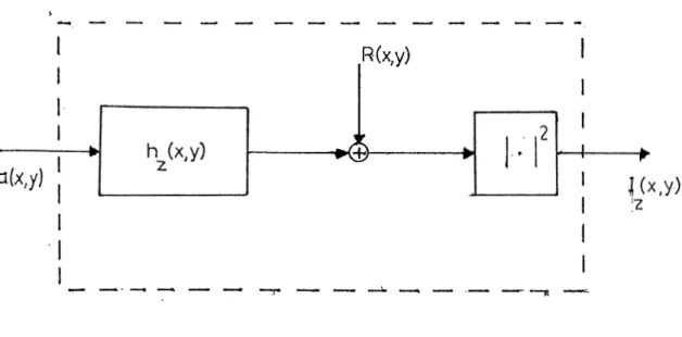
Since the field is represented as a two-dimensional convolution, it can be mod­ eled as the output of a two-dimensional linear system, where the system impulse function is hz{x,y). The block diagram of the system corresponding to hologram recording is shown in Fig.2.2.

CHAPTER 2. MATHEMATICAL MODEL FOR OFF-AXIS HOLOGRAPHY

• 4

R(x,y)

Figure 2.2: Two-dimensional system model for hologram recording

In Eq.2.6, the first term is related to the uniform beam of light and the second ■ term is the cross-term, which is not desirable. The convolution with kernel y)

is an operation which disperses the energy of a space-limited smooth object a(x, y) to a wider region in the x^y plane (wider as 2: becomes large). If the energy of a(x,y) is limited, then the energy of the linear terms in Eq.2.5 drops much below 1. Therefore, the squares of these small values (the cross-term) are negligible. The significant terms are the second and the third terms which contain the factor

a{x,y) and pertain to the image.

2.2.2

R e c o n str u c tio n

The image is reconstructed by illuminating the hologram with a reconstruction beam P{x,y) [4]. This beam is assumed to be a plane wave incident upon the hologram, tilted again only in the .x-direction at an angle $p, as shown in Fig.2.3. If the object is wanted to be reconstructed at its original location, then P{x^y) must be equal to R{x, y), i.e., 9p = 9. From now on we will consider this case only.

CHAPTER 2. MATHEMATICAL MODEL FOR OFF-AXIS HOLOGRAPHY 10

The Fresnel diffraction pattern of the illuminated hologram is

(2.7)

where T{x,y) is a function of I{x,y) depending on the kind of the hologram. In general, holograms can be recorded as amplitude or phase variations [12]. In the amplitude hologram, the interference pattern between the object and the refer­ ence wave is recorded as the amplitude reflection factor of the recording medium. In this case, the fleld after reconstruction becomes

^ r U ^ , y ) = [R(x,y)I(i,y)] · »/¡„(i.ji). (2 .8)

In the phase hologram, the interference fringes are recorded as the variation of the thickness or refractive index of the recording medium. In this case, the field after reconstruction becomes

CHAPTER 2. MATHEMATICAL MODEL FOR OFF-AXIS HOLOGRAPHY 11

^rec(-T,y) = **h^{x,y). (2.9)

For |/(a;,y)| <c 1, the Eq.2.9 becomes

So we can approximate the reconstructed field as

y) = y ) I ( ^ ,»)] * (2.10)

By using Eq.2.10 and Eq.2.6 we can express the field as

'5rec(-'C, y) = ^ y) 4

-R^[^lkxsm(0)\^^^^y>^ ^ */12(3;, y)p] * *h^.{x,y) + * */i’ (a:,y)] * *h^i{x,y) +

Rla{x,y) * *h^{x,y) * *h^.{x,y). (2.11)

If Zi = —z we can simplify Eq.2.11 by using the folloY'ing properties of the convolution kernel h^[x^y') [14]:

(

,

)

h,{x,y) * t k ' ( x , y ) = S(x,y) (2.13)

CHAPTER 2. MATHEMATICAL MODEL FOR OFF-AXIS HOLOGRAPHY 12

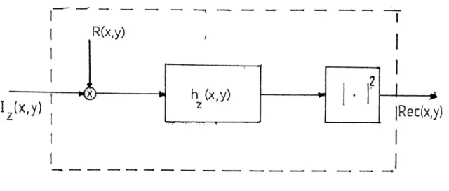
Rec(x,y)

Figure 2.4: Reconstruction from the off-axis hologram Therefore, the field after reconstruction, Trec(3;,y), is

* K { x , y )

» *hl(x,y)

^■Rla(x,y) + * * K ,( x , y ) (2.15)

In Eq.2.15, the first term is the uniform beam of light Avhich propagates straight through the hologram. The second term is the undesired cross term artifact. The third term is the desired reconstruction, and the fourth term is the field of the hologram of the object distribution a(x, y) at a distance 2z and with a shift in the a'-direction.

In some non-optical reconstructions (such as digital) it may be possible to record the held; but in optical reconstruction the magnitude square operation is unavoidable [15].

CHAPTER 2. MATHEMATICAL MODEL FOR OFF-AXIS HOLOGRAPHY 13

As in the recording step, we can model the reconstruction process by a two- dimensional system as in Fig.2.4.

2.3

D isc r e te M o d el

Let’s consider the system given in Fig.2.2. A discrete impulse function hzj^{n,m) must be determined corresponding to the continuous impulse function hz{x, y). In [14] a detailed analysis of sampling of h . ( x , y ) to get /i^p(n,m) is given, so only the results will be mentioned here.

The discrete impulse response hzj^{n, m) is given by

h,^{n,7n) = h , { X n ^ Y m ) if jnj < |m| <

0 elsewhere (2.16)

where iV/i and Mh give the discrete size of the filter in dimensions n and m respec­ tively.

The input function can also be discretized similarly to yield

a£){n^m) = a(Xn,YiTi).

In our implementations, we chose X = Y , i.e., N = M. For the purpose of normalization, a new variable o r , which is related to the sampling of the optical hologram, is introduced [14], such that

a2 JL — JL f2

N X z ^ ■

(2.17)

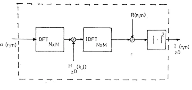
CHAPTER 2. MATHEMATICAL MODEL FOR OFF-AXIS HOLOGRAPHY 14 a (n,m) ► DFT —r<x)—*< I DFT NxM NxM R(n,m). 4 -H (kj) zD

j J (n/n)

Figure 2.5: Discrete implementation of the continuous system given in Fig.2.2

We define another variable ¡5 for the reference beam where

(2.18)

P = 2Tracos{9)J

Now the discrete field can be written as

(2.19)

+ a{n,m) ♦ *h,j^{n,m). (2.20)

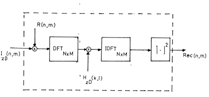
Similar operations can be done for the reconstruction case. In order to increase computational efficiency, circular convolution can be carefully used instead of lin­ ear convolution in Eq.2.20. So we can show the discrete implementations of the continuous systems given in Fig.2.2 and Fig.2.4 as in Fig.2.5 and Fig.2.6.

CHAPTER 2. MATHEMATICAL MODEL FOR OFF-AXIS HOLOGRAPHY 15

Rfrc(n,m )

Figure 2.6: Discrete implementation of the continuous system given in Fig.2.4

2.4

R e su lts

In the simulations, N and M are taken to be 128. Gray level variations are quantized to 256 levels: 0 is the darkest and 255 is the brightest. The amplitude of the reference beam, Ro, is 200 in order to decrease the effect of the cross term in Eq.2.6. At the reconstruction step the DC component is supressed to decrease the effect of the uniform beam of light propagating directly through the hologram.

Fig.2.7 shows a synthesized object and the simulated off-axis hologram of it. If the hologram is reconstructed by using Eq.2.10, w'e get Fig.2.8.

CHAPTER 2. MATHEMATICAL MODEL FOR OFF-AXIS HOLOGRAPHY 16

Figure 2.7: An object and the simulated off-axis hologram of it

7i7.· ..7. ''*A ·

C hapter 3

W AVE P R O P A G A T IO N

3.1

In tro d u ctio n

In this chapter we try to hnd an input-output relationship if we have an array of electrodes, each with a different input, attached to one side of a crystal to form an output surface wave pattern on the crystal.

3.2

P ro p a g a tio n o f an A rb itra ry W ave

If we have a point source located at (xo,J/o) 3,nd oscillating with respect to time as the field on the surface becomes

E (t,r) =

{{x - XoY + { y - Уo)^)^

(3.1)

Now, consider a source whose variation with respect to time is x{t). From Fourier transform relationships, .x(i) can be written in terms of the superposition of complex sinusoids as

CHAPTER 3. WAVE PROPAGATION 18

1

(() = ^ X(w)e’“‘du.

So, by using Eq.3.1 the resultant field of x{t) becomes

1 E o X H

oo ((a; - a-„)2 + (y - y^y)h (3.2)

If we take the constant terms out of the integral and use the Fourier Transform properties (App.A) we get

E{t,r) = Eo 2-k{ {x - X o Y + {y - yoYY ______________ E o 27t((x - XoY + { y - yoY)^ / CO *CO

V E I H E ^ ) .

The above equation shows that the resultant field will be the delayed and scaled version of the input.

3.3

S u p e r p o sitio n o f W aves

As shown in the preceding section, we can find the resultant field due to any arbitrary oscillating source. Now, if we have more than one point source, what will the resultant field be? The answer is the superposition of individual fields, assuming linearity of the media [8].

We will find the actual field at any point by-adding the fields due to each individual source. So, if we have [k + 1) sources located along y and at x = 0 as shown in Fig.3.1, then the total field will be

CHAPTER 3. WAVE PROPAGATION 19

ELEC TRO D ES

Figure 3.1: Superposition of waves

t = 0

here Tj- = + (y — 2/»)^ Vi shows the source location along y.

So

Eo

,-=0 27t(x2 + (y - ViY)^

+ (y - y,)2

i-x(i - --- ). (3.5)

Up to now, we showed how to get the field if we know the source. Now, suppose we know the field. How can we get the source excitations? In order to achieve this, we propose a method which will be studied in the next chapter.

C hapter 4

G E N E R A T IO N OF T IM E SIG N A L S B Y

C O O R D IN A T E T R A N S F O R M A T IO N

4.1

In tro d u ctio n

In this dissertation, we propose a holographic display device where a prescribed surface wave field pattern appears momentarily as a result of the superposition of a number of propagating waves. Each of these waves originates from one of the many electrically excited electrodes attached to the crystal. The forms of the time varying electrode signals are obtained by a mathematical inversion formula from the prescribed field.

4.2

In version R ela tio n sh ip

This section is taken from the US Patent Office Disclosure Document number 225219 [7].

Suppose that our surface is denoted as the plane, with the upper left corner being the origin. We locate electrodes on the y-axis. From now on, assume

CHAPTER 4. GENERATION OF TIME SIGNALS BY COORDINATE TRANSFORMATION 21

the variation along the y-axis is continuous, so the applied signal is given by a two-dimensional function After finding the result for the continuous case, it can be easily discretized.

Let the time varying field on the crystal surface be tj;t(x,y). At a specific instant of time i,· we want to find the electrode signals, f ( t , y ) , from the surface pattern, !/)(,.(a;, y).

Consider a general propagating plane wave which can be written as

where, k is the wavenumber vector (¿i, ky)'^, and, x is the position vector (a:,y)^. The direction of propagation is given by a = ( ^ , ^ ) ^ · The speed of propagation is pj·.

|o|

Now, let the wave be multiplied by a linear phase component e·’“'·*' at the crys­ tal edge. This is analogous to the diffraction of light through a prism, or by a sawtooth transparent phase grid. For a wide range of u, the plane wave continues its propagation after the edge, on the crystal surface, but now it is refracted by a linear phase component. Therefore, if the signal

is applied to the electrodes, then there will be a time-varying field over the crystal surface as

g j { u i t - k x X + u y )

This field is shown in Fig.4.1 where u = 0.3.

As stated above, for this field to continue propagation on the crystal, u should satisfy the constraint shown below.

speed = u

CHAPTER 4. GENERATION OF TIME SIGNALS BY COORDINATE TRANSFORMATION 22

Figure 4.1: Time-varying field at i = 0

We know the wave number in the y-direction from the excitation as ky -u.

So, U) ■ J W + (4.2) which yields kx - 10 \ u" to u (4.3)

If I u |> | A: 1= then this argument is no longer valid, since in this case the wave will not propagate on the crystal surface.

As stated above, we have the two-dimensional ..time-varying surface field at a specific instant of time t,·, i.e..

CHAPTER 4. GENERATION OF TIME SIGNALS BY COORDINATE TRANSFORMATION 23

(4.4)

From this field we want to get f { t , y ) . So our problem reduces to a two- dimensional transformation. Considering the (i, y) domain as the input domain, and the (x,y) domain as the output domain, we want to transform ^'i,(x,y), the surface field, to /( i,y ) , the electrical signals applied to the electrodes. In other words, we want to get a sinusoidal input at the (i, y) domain with frequencies u> and

u respectively, from the sinusoidal output at the (x,y) domain with 0.x = —kx and Q,y = —ky. To find this transformation we use the well-known Fourier transform

relationships[2],[3].

Suppose we want to generate an arbitrary field distribution We can easily decompose this two-dimensional signal into its sinusoidal components using the Fourier transform as

1 /‘ + CO r+oo ,

. ( ^ . » ) = Tt / / (4.5)

47T J - o o J - c o

The complex weights can be found from the Fourier transform as

/ + 00 r + oo .

/ i/’i.(a:,y)e“^“^®e"·’ ^^dxdy.

- C O J- o o

(4.6)

We have shown previously that in order to get a surface field pattern ipti{x·, y) — .yyg ]iave to apply f { t , y ) = to the electrodes.

So, in order to get we must apply to the electrodes. Finally, it can be argued that

CHAPTER 4. GENERATION OF TIME SIGNALS BY COORDINATE TRANSFORMATION 24

where is a constant for fixed Q,x and Qy.

Therefore, in order to get the arbitrary surface field pattern

/ ‘ + C O r + co I r-roo r-too 4 /1 J — oo J — oo we must have 1 r+<x> r + c a O O J —oo 4?!^ J- (4.7)

From Eq.4.2 we know that

Hence, or, équivalent^, oj 1= c^Jkl + k^. u> =_ / if Q. < 0 - ^ \A F + ~ ^ if fix > 0 (4.8) n UJ = n . ^ c y / n j + n ;. (4.9)

The reason for the change in the sign of a; due to is that the wave propagates away from the excitation electrodes, i.e., always in the positive x’-direction.

CHAPTER 4. GENERATION OF TIME SIGNALS BY COORDINATE TRANSFORMATION 25 /( i.y ) 4 7 T ^ j —oo J —oo 2 f-l·oo /*+co 47T^ / i - C O /*-t-CO / « .,( -C O J —oo — a; (jü^ U) iiy) - CJ

c’V 5 ^

/ ■ ^ -c o f + C O

/ F{0J,u)e^‘^^e^'^^dudu. -OO j — CO

(4.11) As a result if we compare Eq.4.10 and Eq.4.11 we get

F{co,u) |^^nj,= ^ i.(— \ LO \ U)^

to - n j . n , ) ·

- ( J j

V #

(4.12) where F{co, u) and ^¿,.(51(0;, u), u) are the Fourier transforms of f ( t , y) and y)

respectively.

Therefore we can always find the unique input signal /(¿, y) in order to get the specified surface field pattern V’<¡(^)2/) timet,·, and the relationship between the Fourier tran.sforms of these two signals is as given above.

If we look at the above equations carefully we see that the bands of F'(tu, u) and T<, (5'(o.', u),u) are not the same. The relationship can easily be found analytically or graphically. Fig.4.2 shows an example: is a bandpass signal with a rectangular passband, and the corresponding passband of f { t , y ) is shown in Fig.4.3. As shown previously, the coordinate transformation is valid only for Iu| >

After the coordinate transformation we see that the band is hyperbolaid. Fig.4.4 and Fig.4.5 show the reverse coordinate transformation, i.e., the coor­ dinate transformation from a rectangular passband in the (w, u) domain (Fig.4.4)

CHAPTER 4. GENERATION OF TIME SIGNALS BY COORDINATE TRANSFORMATION 26

lx

1

fly

Figure 4.2: with a rectangular pass-band. (Taken from [7] with the permission of the author)

lw| = c lu|

<|=fly

Figure 4.3: F{lo,u) after coordinate transformation. (Taken from [7] with the

CHAPTER 4. GENERATION OF T M E SIGNALS BY COORDINATE TRANSFORMATION 27 W i i 1 u = Ry .Ay

Figure 4.5: after inverse coordinate transformation. (Taken from [7] with the permission of the author)

CHAPTER 4. GENERATION OF TIME SIGNALS BY COORDINATE TRANSFORMATION 28

to the (Í2x,fíy) domain (Fig.4.5).

4.3

D ig ita l P ro c essin g

The inversion relationship between the source signal f { t , y ) and the surface field

xl>t{x,y) is given in the previous section as a transformation between the Fourier

domains (cu,u) and In practice the length of the crystal edge where the sources are located is finite; the source is not continuous but a discrete array. In digital processing, the input surface wave pattern and the output surface wave pattern are also discrete.

Let us denote the discrete surface wave pattern as for n = 0...N — l,m = 0...M — 1, and the discrete excitation signal by /( a , b) for a = O...A^' —1, b =

0...M' — 1. One can take the DFT (Discrete Fourier Transform) of to get Tt,-^(^,/) as in Eq.4.13

A '-l M-1

(4.13) n=0 m=0

where k = 0...iV — 1, / = 0...M — 1.

If there is no aliasing, the elements of this two-dimensional array are the sam­ ples of the continuous Fourier transform Knowing these samples, which are located on a rectangular grid, we can also find the samples of the F{io, u) through the relation 4.12

^ u i U k . V l ) -\U k\ cUk Uk ^ / Î T W T V W -\Uk\ cUk Uk ^ / U W T W P F { - ^ cV Ï P ¥ T V ^ , VI) F { k \ r ) . (4.14)

CHAPTER 4. GENERATION OF TIME SIGNALS BY COORDINATE TRANSFORMATION 29

Ay

Ax

n y

Figure 4.6: Sample locations after and before transformation

where 0 < k* < N', 0 < I* < M'. U and V are the sampling periods, c is the propagation speed of the wave, N ' and M ' are given by Eq.4.15 and Eq.4.16:

N ' = c-Ju’‘( N - I P + V^(M - 1)2, (4.15)

M' = V ( M - 1). (4.16)

However, the sample locations in this case do not form a rectangular grid. The locations are shown in Fig.4.6. In order to use an inverse DFT to get the discrete time signals, uniformly sampled data is required; i.e., we have to know i^(d, e) for d = 0, — \ and e = 0, — 1.

CHAPTER 4. GENERATION OF TIME SIGNALS BY COORDINATE TRANSFORMATION 30

This can be achieved rather easily, because the sampling in the u-direction is already uniform. A column of points, corresponding to a constant k = e (or equivalently to a constant u) can be taken at a time, digitally interpolated by a sufficient amount first and then sampled again to get the samples of F{u>, u) at the proper locations to form a rectangular sampling grid. Of course, the interpolation is different for each e.

After interpolation and resampling, taking the inverse DFT of F (d, e) for d = 0...N' — 1, e = 0...M ' — 1 will give us the discrete time signals f(a, b) where

N ' - l M ' - l

f[a,b) = E F{d,e)e~^

n =0 m=0

(4.17) for a = 0...N' - 1 . 6 = - 1.

As we use DFT in computations, the time signal /( a , b) formed in simulations is intrinsically periodic in both a and b directions (Eq.4.18 through Eq.4.20). But the inversion relationship between the surface field and the time signal is derived in the continuous domain (Eq.4.12) and because of this, the time signal is of infinite extent in both variables t and y. This causes aliasing in the computed periodic time signals. The effect of aliasing can not be gotten rid of but can be decreased by zero padding the input image

^{u>x,cjy) (4T8)

where is the discrete-time Fourier transform of the finite support input image, m); i.e.

CO CO

n = - c o m = —00

As we are working in discrete domain we need the samples of Sam­ pling in frequency domain yields periodic repetition of in space domain as given by Eq.4.19.

CHAPTER 4. GENERATION OF TIME SIGNALS BY COORDINATE TRANSFORMATION 31

'P(&,/) = 4=^ ^ ^ nг + M j) (4.19)

i 3

where N and M are the periods.

After coordinate transformation given by Eq.4.14 we get

F(d, e) = F(w, + N'i, b + M'j). (4.20)

As we have a periodic input pattern given by the righthand side of Eq.4.19, the time signal that must generate it must also be periodic as given by the righthand side of Eq.4.20, but we have overlaps in the time signal. The reason for these overlaps is the infinite extent of the time signal in both variables t and y. If one wishes to have a perfect reconstruction of the periodic pattern,

J2i i^{n + N i , m M j ) , then an infinite array of electrodes all radiating at all

times must be considered. However, we must restrict ourselves to a finite number of electrodes, i.e. a finite number of periods of the time signal in y-direction. If only one period (in y-direction) of the time signal is chosen, then all of the 2- D periods of the space pattern degrades but the degredation is less in the main period. The degredation is due to information missing because of not using all the periods.

Even though we can get a perfect reconstruction by using an infinite array of electrodes we can not get rid of the aliasing effect due to the infinite extent of the time signal. This effect can be decreased by proper choice of N and M, i.e. by zero padding the input pattern as given by Eq.4.24. If we choose N and M large enough we get

CHAPTER 4. GENERATION OF TIME SIGNALS BY COORDINATE TRANSFORMATION 32

for the main period. So the time signal required to generate this pattern is also more concentrated on the main period.

The above procedure is implemented by using SUN workstations as follows:

• The first step is to zero pad the input image, the image which will be on the crystal at a given instant as a result of the propagation of the electrode signals, and take the 2-D N x M discrete Fourier transform. The Fourier transform is taken by using a Radix 4 transform (App. B). The real and imaginary parts are stored separately.

• If the original signal has a DC value, it must be supressed because the magnitude after the coordinate transformation blows up to infinity on the |u| = |a^|/c lines which correspond to = 0 (Eq.4.12). Let us denote this lower cut-off frequency as “/iou;·”

• Now the coordinate transformation given by Eq.4.14 can be done. As stated previously, after the coordinate transformation we will have no more uniform samples. So, interpolation and resampling must be done.

Various interpolation algorithms are found in literature for both nonuniform and uniform samples [1],[5],[6],[16],[17]. The interpolation algorithms for uniform sampled data are much easier and more efficient to implement. So, in this step we did the interpolation between the samples of T(A:,/) which are known on a uniform rectangular grid.

In the discrete domain Eq.4.9 becomes

rC (4.21)

where i/, V are the sampling periods and c is the speed of propagation. The constant c is chosen such that the DFT size does not change after the coordinate transformation, i.e., N = N', M = M'.

By using Eq.4.21 we can find dmin and .where d^in — c.liow and dmax =

c^U.U.Nl2.Nl2 + V.V.MI2.MI2 as k = N/2,1 = M / 2 corresponds to the

CHAPTER 4. GENERATION OF TIME SIGNALS BY COORDINATE TRANSFORMATION 33

Now, we want to find the value of F{k, 1) at each I for kmin ^ k < kmax·

For this, we perform the inverse coordinate transformation to find the cor­ responding value in the (¿, 1) domain as

(4.22) where 0 < k' < N. As seen from Eq.4.22 the k' may not be an integer. Since the pixel values are defined only at integer values of k and I, using non­ integer values causes a mapping into locations of for which no gray levels are defined. It then becomes necessary to infer what the gray level values at those locations should be, based on the pixel values at integer coordinate locations by using interpolation.

The interpolation that we used here is a combination of linear interpola­ tion and resampling as described below [1]. There are other interpolation algorithms in the literature [5j,[6],[16],[17].

- Compute the 2-D inverse DFT of the finite size sequence T(^, 1) of size

N x M in order to get x/;(n,m) for n = Q..N — l,m = 0..M — 1

1 N-\ M-l

S (4.23)

k=0 1=0

- Zero pad tp(n,m) and construct a new sequence i/^new{n,m) as follows:

Tp{n.,m) n = 0,..., A^/2; m = 0,..., M — 1 i^{n + N - LN, 77i) 7i = L N - N / 2 + 1 , . . . , L N - 1 ] m — 0,..., M — 1 0 n = A^/2-f l,...,T iV -iV /2 ; m = 0,..., M — 1 (4.24) Perform 2-D DFT on the sequence il}new{n,m) to obtain the sequence

CHAPTER 4. GENERATION OF TIME SIGNALS BY COORDINATE TRANSFORMATION 34 Figure 4.7: Interpolation 1 L N M ¡_Q where knew = 0 ,. .., LN - 1,1 = - 1. (4.25) 'i(^'neu,,0 = 0 for k„.new > L N - 1

The above operation is equivalent to upsampling by L and filtering of

'^{k, 1) along the ¿-axis in order to get more samples in this dimension

[6]. The upsampling ratio is limited by the size of the arrays that can be used in SUN-workstations. The arrays which are of float type can use 8 megabytes of swap area which is the actual swap area of the system. Although 2-D DFT interpolation increases the sampling rate signifi­ cantly, further interpolation is needed for coordinate transformation. So, at this step we perform an additional linear interpolation. The weighted average of two nearest neighbors along ¿-direction, along which there are no electrodes, is taken as follows.

CHAPTER 4. GENERATION OF TIME SIGNALS BY COORDINATE TRANSFORMATION 35 /) = + 1 - k'\ + i(l-i + 1, i) |ii - k'\ (4.26) where k\ ^ Z k' = - a R a U k\ k <C "h 1.

• After this interpolation scheme we get F{d, e) for each d, e in the region bounded by e^tn < e < ^max-i Limits of d do not change.)

• Now we have i^(c, d) which consists of uniform samples so we can take Inverse Discrete Fourier Transform. The result of Inverse Discrete Fourier Transform will give us the samples of / ( i, y)

1

= 1517 E E

w'here a = 0,..., — 1,6 = 0,..., M — 1.

(4.27)

4.4

R esu lts

In our simulations we chose the size of the object to be 64x128, the upsampling ratio L to be 4, the propagation speed c to be 1.0 and the sampling periods U and

V to be 1.

The algorithm was applied to various images. The series of simulations shown in Fig.4.8-4.12 show the effect of spurious response due to the periodicity of the com­ puted time signals. Fig.4.8 is the original input pattern. Fig.4.9 is the computed time signals when the input object is extended to a 128x128 image by zero-padding

CHAPTER 4. GENERATION OF TIME SIGNALS BY COORDINATE TRANSFORMATION 36

and Fig.4.10 is the one when the input object is extended to a 256x256 image again by zero-padding. When these time signals are radiated we get Fig.4.11.a and Fig.4.11.b respectively. The effect of periodicity on the reconstructed pattern can easily be seen from these figures. When we pad the input pattern by more zeros we decrease the effect the portion of the time signal which causes aliasing; i.e. the portion of the time signal related to the other periods of the input image. As the whole information about the input object forms only a small portion of the input pattern after zero padding, the related time signal has also most of the information concentrated in a limited region. We can still get a better reconstruc­ tion by using more than one period of time signal in radiation. As each period contains extra information, when the number of periods in radiation increases, our approximation converges to the ideal case where the time signal is of infinite length and the pattern generated by the radiation of this time signal is the periodically repeated version of the input pattern. Fig.4.11.c shows the reconstructed pattern where 5 periods of the time signal in y-direction are used in radiation. The time signal is repeated in ¿-direction until the input pattern is generated as in the pre­ vious cases. When the number of periods increases we get a better reconstruction but the computation time increases enormously.

Two other series of simulations are shown in Fig.4.12 through Fig.4.15.

Fig.4.16 through Fig.4.21 show the relation between the number of electrodes and resolution. The two points in Fig.4.16 are one pixel apart from each other. Fig.4.17 is the time signal for 128 electrodes, and Fig.4.18 is the time signal for 256 electrodes. When these time signals are radiated we get Fig.4.19 and Fig.4.20, respectively. It is seen from Fig.4.19 to Fig.4.20 that we can get the resolution given in Fig.4.16 by using 256 electrodes.

The output images are shown using a common intensity scale and each point is represented by an 8-bit intensity level.

CHAPTER 4. GENERATION OF TIME SIGNALS BY COORDINATE TRANSFORMATION 37

Figure 4.8: luput object pattern

CHAPTER 4. GENERATION OF TIME SIGNALS BY COORDINATE TRANSFORMATION

! i E @ l

38

Figure 4.10: Computed time signals after e.xtension to 256x256 image

.[ T » wiT'V" fflw .m y ? ;

Figure 4.11: Reconstructed objects (a)by radiating the time signal in Fig.4.9,(b)by radiating the time signal in Fig.4.10, (c)by periodically radiating the time signals in Fig.4.10

CHAPTER 4. GENERATION OF TIME SIGNALS BY COORDINATE TRANSFORMATION 39

Figure 4.12: Input object pattern and reconstructed object after radiation of time signal in Fig.4.13

CHAPTER 4. GENERATION OF TLMB SIGNALS BY COORDLNATE TRANSFORMATION 40

...

t ' j . A . >< , ' ’^^.*1·) ] i , , · ' . . ’■'„r-v;

L'';i'&' pr-LY "'X VSW

Figure 4.14: Another input object pattern and reconstructed object after radiation of time signal in Fig.4.15

CHAPTER 4. GENERATION OF TIME SIGNALS BY COORDINATE TRANSFORMATION 41

Figure 4.16: Input pattern to show the relation between the resolution and the electrode number

CHAPTER 4. GENERATION OF TIME SIGNALS BY COORDINATE TRANSFORMATION 42

Figure 4.18: Computed time signals for 256 electrodes

CHAPTER 4. GENERATION OP TIME SIGNALS BY COORDINATE TRANSFORMATION 43

C hapter 5

A P R A C T IC A L IM P L E M E N T A T IO N

The algorithms presented in the previous sections can be used to develop a three- dimensional acousto-optic television display [7].

The principle of operation is based on forming the holographic pattern, for a short duration of time, on a crystal using propagating surface waves, and illumi­ nating the so-formed hologram at the proper instant by a coherent light pulse to reconstruct the associated wavefront which yields a three-dimensional frame.

The propagating surface waves are generated by a number of electrodes on one side of the crystal. The electrical signals applied to these electrodes are derived from the desired hologram pattern using the inversion relation presented in Chap.4. Consecutive frames can be written easily on the crystal, and with a proper rate of repetition, a continuous three-dimensional motion picture can be observed.

In Fig.5.1, a possible three-dimensional holographic television system which utilizes the above technique is shown. At the transmitter side, there is a video camera 1 which captures the two-dimensional hologram pattern in front of it. The hologram represents the three-dimensional scene as seen by the camera. The

y

hologram pattern captured by the camera is converted into electrical video signal and then transmitted through a channel 2 to the receiver. The received video signal

CHAPTER 5. A PRACTICAL IMPLEMENTATION 45

ELECTRODES

Figure 5.1: A practical implementation

SAW

LIGHT SOURCE

is then processed by the block labeled “processor” 3. This processor performs the previously mentioned mathematical inversion processes to get the electrode signals. These electrode signals then generate the time-varying field pattern on the crystal surface, which is indeed a surface acoustic wave device (SAW) [20]. The time- varying field will yield a reproduction of the hologram in front of the video camera at a time instant to- Right at this time, a pulse of coherent light, may be from a laser 4, is passed through the crystal, to reconstruct the three-dimensional scene, seen by the camera, in front of the observer 5. Since there is no need to erase the written hologram explicitly, the system is ready for another frame in a short time where this duration is limited only by the propagation speed of the surface waves on the crystal. If consecutive frames are sent frequently enough, as in conventional television, the observer will see a three-dimensional motion picture.

C hapter 6

R ESU LTS

The simulation of three-dimensional holographic television display was carried out by using the algorithms given in the previous chapters for various input patterns.

Fig.6.1 shows the 64x128 2D flower pattern, a(n,m) and the simulated holo­ gram of this pattern. Fig.6.2 is the time signal generated by using the method described in Chap.5. Here, the vertical axis is the “electrode axis”, whereas the horizontal axis is time. If these signals are applied to the electrodes, the propa­ gating waves from each electrode will superpose to generate the pattern shown in Fig.6.3 at a specific instant. Here, the desired result is to have Figures 6.1.b and 6.3 exactly equal to each other. However, due to propagation (and some compu­ tational errors such as round off noise) the two pictures will be slightly different. Using this new pattern as the hologram (which would be on the surface of the SAW -surface acoustic wave- device), the original object (which is a 2-D, i.e., flat pattern in 3-D space for this figure) can be reconstructed as in usual holography. This will be done optically in the real system, but here the reconstruction result is obtained through simulation. This is shown in Fig.6.4.a. For comparison, the same simulation method is applied to the original hologram of Fig.6.1.b. The result of this simulation is shown in Fig.6.4.b.

<f

Another series of images are shown in Figures 6.5-6.8. In these simulations.

CHAPTER 6 . RESULTS 47

the input images are first extended to 256x256 images and 5 periods of generated time signals for 256 electrodes are used in reconstruction.

A series of simulations shown in Fig.6.9-6.13 are different. The simulated object in this case is 3-D: there are two squares (each is a 2-D object), but they are located at different depths (the third dimension). Again, the reconstructions are simulated both from the original hologram and the hologram obtained from the propagation of the acoustical waves from the electrodes. Since there are two different depths, two different reconstructions, each focusing at a different object are shown. The results are very satisfactory.

The simulations were carried out by using SUN-3/110 deskside color worksta­ tion which is a 32-bit system based on Motorola MC68020 CPU chip and the high­ speed 32-bit VME bus. The operating system is the enhanced version of UNIX. The main memory is eight megabytes and there are 256 simultaneously displayed colors. The hardware also includes a coprocessor MC6881. The system has a window-based user environment to exploit the capabilities of the high-resolution 1152x900 bit-mapped screen. The display of gray level images is performed by using the windows and pixwins (related to pixels) to access the specific portion of the screen defined by windows.

The simulation programs were written in C, which is a general purpose lan­ guage, designed for structured programming. For display purposes, the results of the computations are converted to 256 gray level images. For all of the pictures, this is done by assigning the lowest pixel value to 0, and the highest one to 255. This assures the maximum use of the dynamic range of the gray image.

CHAPTER 6 . RESULTS 48

Figure 6.1: (a)The 64x128 2D flower pattern and (b)the simulated hologram of this pattern

CHAPTER 6. RESULTS 49

Figure 6.3: The reconstructed hologram after radiation of time signal in Fig.6.2

CHAPTER- 6 . RESULTS 50

Figure 6.5: (a)Anotlier input pattern and (b)the simulated hologram of this pat­ tern

CHAPTER 6 . RESULTS 51

Figure 6.7: The reconstructed hologram after radiation of time signal in Fig.6.6

7

CHAPTER 6 . RESULTS 52

' ’ ‘ · ■■ L' ,

Figure 6.9: (a)A 3D input pattern and (b)the simulated hologram of this pattern

CHAPTER 6 . RESULTS 53

-J: .

H

Figure 6.11: The reconstructed hologram after radiation of time signal in Fig.6.10

T".

u y^ vi-># " -^ v m a C ' ·*»> K·*

^ ; : ^ t ' . i u t 1 ’ii‘t ' · · fli.

Figure 6.12: Reconstruction of the two objects ^at different depths from the holo­ gram in Fig.6.9.b

CHAPTER 6 . RESULTS 54

Figure 6.13: Reconstruction of the two objects at different depths from the holo­ gram in Fig.6.11

C hapter 7

H O W TO U S E T H E SIM U L A T O R

The simulation programs implement six different tasks such as system function generation for holography, conventional off-axis holography, reconstruction from hologram, time-signal generation, wave propagation on the crystal and the display of the created images.

All the programs have standard input/output formats which have four bytes of header in front of the actual floating-point data. The header contains the input data sizes of the x and y coordinates. The programs are interactive. They all ask for inputs such as filenames and certain parameters by prompting with a suitable explanation.

7.1

E xam ple

Suppose that the image file o b je c t.im g has already been generated by using the standard input/output format found in SUN workstations (App. C). In order to take its hologram, to find the time signals and to radiate them, to reconstruct the object back and to display the resultant images the following sequence of main programs must be executed.