RESEARCH ARTICLE
10.1002/2013SW000998 Key Points:• Online, automatic, slant total electron content is computed as IRI-Plas-TEC • IRI-Plas-STEC is available from www. ionolab.org for desired date, hour, and location
• IRI-Plas-STEC is provided via e-mail in both graphical and text format
Correspondence to:
H. Tuna,
Citation:
Tuna, H., O. Arikan, F. Arikan, T. L. Gulyaeva, and U. Sezen (2014), Online user-friendly slant total electron content computation from IRI-Plas: IRI-Plas-STEC, Space Weather, 12, 64–75, doi:10.1002/2013SW000998.
Received 3 OCT 2013 Accepted 26 DEC 2013
Accepted article online 6 JAN 2014 Published online 24 JAN 2014
Online user-friendly slant total electron content computation
from IRI-Plas: IRI-Plas-STEC
Hakan Tuna1, Orhan Arikan1, Feza Arikan2, Tamara L. Gulyaeva3, and Umut Sezen2
1Department of Electrical and Electronics Engineering, Bilkent University, Ankara, Turkey,2Department of Electrical and
Electronics Engineering, Hacettepe University, Ankara, Turkey,3IZMIRAN, Moscow, Russia
Abstract
Slant total electron content (STEC), the total number of free electrons on a ray path, is an important space weather observable. STEC is the main input for computerized ionospheric tomography (CIT). STEC can be estimated using the dual-frequency GPS receivers. GPS-STEC contains the space weather variability, yet the estimates are prone to measurement and instrument errors that are not related to the physical structure of the ionosphere. International Reference Ionosphere Extended to Plasmasphere (IRI-Plas) is the international standard climatic model of ionosphere and plasmasphere, providing vertical electron density profiles for a desired date, time, and location. IRI-Plas is used as the background model in CIT. Computation of STEC from IRI-Plas is a tedious task for researchers due to extensive geodetic calculations and IRI-Plas runs. In this study, IONOLAB group introduces a new space weather service to facilitate the computation of STEC from IRI-Plas (IRI-Plas-STEC) at www.ionolab.org. The IRI-Plas-STEC can be computed online for a desired location, date, hour, elevation, and azimuth angle. The user-friendly interface also provides means for computation of IRI-STEC for a desired location and date to indicate the variability in hour of the day, elevation, or azimuth angles. The desired location can be chosen as a GPS receiver in International GNSS Service (IGS) or EUREF Permanent Network (EPN). Also instead of specifying elevation and azimuth angles, the user can directly choose from the GPS satellites and obtain IRI-Plas-STEC for a desired date and/or hour. The computed IRI-Plas-STEC values are presented directly on the screen or via e-mail as both text and plots.1. Introduction
The ionosphere is a layer in the atmosphere which lies in the altitudes ranging from about 90 km to 1000 km. Ionosphere is distinguished from other layers of the atmosphere because it is ionized mainly by solar radi-ation. It has crucial importance in satellite communication because of its conductive, inhomogeneous, anisotropic, temporally and spatially varying, and temporally and spatially dispersive nature.
The most important parameter for modeling the ionosphere is the electron density profile which is a direct way to investigate the structure and variability of the ionosphere as well as the ionospheric influence on radio waves. Radio waves are reflected and/or refracted as they travel through ionosphere based on the electron density distribution in the layers of the ionosphere.
Total electron content (TEC) is defined as the line integral of electron density on a given ray path. TEC cor-responds to the total number of free electrons in a cylindrical path with a 1 m2cross-sectional area, and it
is widely used in space weather studies for investigation of ionospheric variability. The unit of TEC is TECU where 1 TECU is equal to 1016electrons/m2. When TEC is calculated on a vertical path in the local zenith
direction, it is called vertical total electron content (VTEC). Slant TEC (STEC) is usually used to designate the total number of electrons on a ray path other than the local zenith direction.
Ionosphere is the main source of error for Global Navigation Satellite Systems (GNSS) due to its highly vari-able structure, and it causes unpredictvari-able time delays. Without calculating the ionospheric delay and inserting it into their measurement models, GNSS systems can not obtain high-resolution position esti-mates. The widely used Global Positioning System (GPS) provides a cost-effective means for computation of STEC (GPS-STEC) using pseudorange and phase delay recordings of dual-frequency Earth-based receivers [Komjathy, 1997; Schaer, 1999; Davies and Hartmann, 1997; Arikan et al., 2003]. GPS-STEC is used both in correction of positioning errors due to ionospheric delays and also in ionospheric physics to capture the underlying structure of ionosphere using computerized ionospheric tomography such as in Erturk et al. [2009], Sibanda [2010], Jin and Jin [2011], and Hirooka et al. [2012]. The GPS-STEC measurement model
includes instrumental biases that need to be determined to increase the positioning resolution and reduce nonionospheric components from STEC. Unfortunately, due to ambiguities and uncertainties, GPS-STEC can never be obtained in such a way to represent ionospheric and plasmaspheric part alone [Komjathy, 1997;
Schaer, 1999; Arikan et al., 2008].
There are approaches in the literature for calculation of STEC values by using an ionosphere model. Gener-ally, thin-shell approximation is adopted and STEC values are related to the VTEC values with an obliquity factor [Lanyi and Roth, 1988; Manucci et al., 1998; Mushini et al., 2009]. Thin-shell method is an oversim-plified approximation method that ignores the inhomogeneous structure of the ionosphere. In order to take into account the variation of electron density along the ray path, line integration methods are gener-ally used such as in Cabrera et al. [2005] and Nava et al. [2008]. In Cabrera et al. [2005], the electron density profile along the slant path is obtained from International Reference Ionosphere (IRI) [Bilitza, 2001] and Chapman models with 20 km segments, and integrated electron density values are computed between 50 km and 2000 km. In Nava et al. [2008], a method for fast computation of STEC values is introduced where electron density values are obtained from NeQuick2 model, which is an updated version of the NeQuick ionosphere model [Radicella, 2009]. The numerical STEC computation based on NeQuick2 is provided as an online tool available at “http://t-ict4d.ictp.it/nequick2/nequick-2-web-model.” On the website, STEC path can be defined by latitude, longitude, and height. The lower end can also be obtained using the cursor posi-tion and online map, and higher end can be defined using the satellite posiposi-tion in azimuth, elevaposi-tion, and height. Year, month, and time are the temporal variables. Solar activity can be provided by the user, or it can be chosen from recorded values. The STEC values are computed using the model electron density values in
Nava et al. [2008], and the output is provided in a text file on-screen, providing the electron density along
the ray path. The electron density profile is also plotted in a graph in jpeg format. The major drawback of IRI and NeQuick electron density profiles is the modeling of topside ionosphere and plasmasphere [Coïsson
et al., 2006].
In order to overcome the modeling difficulties of electron density in plasmasphere, IRI model is recently modified into International Reference Ionosphere extended to Plasmasphere (IRI-Plas) to extend the height coverage to GPS satellite altitude of 20,200 km [Gulyaeva, 2010]. In IRI-Plas, the electron density values are obtained by an updated-scale parameter set [Gulyaeva et al., 2011; Gulyaeva, 2012]. IRI-Plas model gives greater proximity to real measurement values [Maltseva et al., 2013; Gulyaeva et al., 2013] and is recently designated as the international standard model for ionosphere and plasmasphere [Gulyaeva and
Bilitza, 2012].
In this study, a new IONOLAB online user-friendly STEC calculation tool is introduced at www.ionolab.org website. This unique IONOLAB service utilizes IRI-Plas model and line integration method for STEC calcula-tion and presents a web-based service with comprehensive features. The ionosphere and plasmasphere are divided into horizontal layers by using preset altitude step sizes. Small altitude step sizes are used for high electron density regions, and larger altitude step sizes are used for low electron density regions. The alti-tude values extend from 100 km to 20,000 km, which covers the plasmasphere and the ionosphere. For a given slant path, the spherical coordinates of the points where the slant path reaches the mean altitude of these layers and the length of the slant path within the corresponding layers are calculated. The electron density values at the calculated locations on the propagation path are obtained from IRI-Plas model for the default climatic ionospheric parameters, which would provide us the climatic component of STEC. Electron content contribution at each layer is calculated by multiplying the electron density values and the length of the propagation path within the corresponding layer. Finally, STEC values are calculated as the summa-tion of these electron density contribusumma-tions. By changing the input parameters and repeating the same procedure, variation of STEC with respect to hour, satellite elevation angle, and satellite azimuth angle can be generated.
In IRI-Plas-STEC web service, the electron density values along the chosen ray path can be obtained for a desired location, date, hour, elevation, and azimuth angle. The computed STEC value is provided as a num-ber in TECU. The electron density profile values along the ray path are also given in a text file on-screen. The variation of STEC with respect to hour in a day, elevation angle, and azimuth angle can also be observed for a desired location and date. Since these options require multiple STEC calculations, computation time increases. Therefore, when they are ready, computed results are sent to the user via user-defined e-mail address as an attachment. In the attachment, both the computed STEC values and its graphical
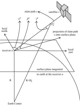
Figure 1. Slant path geometry and STEC calculation parameters.
representation are given. In the future, to obtain near-real-time results, it is planned to provide an option of performing STEC computation by using coarser discretization of the line integrals. In order to facilitate the comparison of model-based IRI-Plas-STEC with measurement-based GPS-STEC values, the desired location can be chosen from International GNSS Service (IGS) stations [International GNSS Service, 2013] or EUREF Per-manent Network (EPN) stations [EUREF, 2013] using the four-digit GPS station codes or selecting from the provided IGS station map. Also to define the upper end of the STEC ray path, any desired GPS satellite can be chosen online through the Pseudorandom noise (PRN) identification numbers. For the chosen GPS satellite, either a STEC value for the given hour is computed or the value of STEC on the satellite path is computed for the given day and provided in a plot. These unique computational capabilities enable users from various disciplines to observe model-based variability of STEC in time, elevation, and azimuth.
In section 2, proposed STEC calculation method from IRI-Plas model is explained. In section 3, STEC calculation service is presented.
2. STEC Calculation From IRI-Plas
In this section, the mathematical details of STEC computation are provided. The parameter s indicates the slant path along which STEC to be computed as given in Figure 1. In order to calculate the STEC along a given slant path s, the coordinates of the points on the slant path s and the electron density values at the corresponding locations from IRI-Plas model are required.
A slant path s can be uniquely defined as the propagation path between receiver u and satellite v, for a given time t. The coordinates of the slant path s and the slope of the slant path s are calculated for discrete height values contained in array H in increasing order. In the following calculations, Hirepresents the ith height
level in array H and Ps
irepresents the point where slant line s reaches height Hi. The Earth is considered as a
sphere with a radius of 6378 km, which will be denoted as R. Before beginning calculations, suppose that, the parameters listed in Table 1 are given as input parameters.
Let𝛾s
i represent the angle between the slant path s and the surface normal, which intersects s at point P s
i,
and let Ds
irepresent the distance between the receiver u and the point P s
Table 1. Input Parameters for Calculating the Slant Path Coordinates
Symbol Definition
𝜙(u) Latitude of Receiveru
𝜆(u) Longitude of Receiveru
𝛼s Satellite Elevation Angle
The angle between the surface plane at the receiverulocation and the slant paths
𝛽s Satellite Azimuth Angle
The clockwise angle between the local north vector at the receiverulocation and the projection of the slant pathsonto the surface plane which is tangential to Earth at the receiverulocation
of cosines,𝛾s iand D
s
ican be calculated as follows:
𝛾s i = sin −1 ( R R + Hi sin( 𝜋 2 +𝛼 s)) , (1) Ds i = √ R2+(R + H i )2 − 2R(R + Hi ) cos( 𝜋 2−𝛼 s−𝛾s i ) . (2) After Ds
iis calculated, the local east, north, up (ENU) coordinates of the point P s i can be calculated by using (3). ⎡ ⎢ ⎢ ⎣ E(Ps i) N(Ps i) U(Ps i) ⎤ ⎥ ⎥ ⎦ = ⎡ ⎢ ⎢ ⎢ ⎣ Ds icos (𝛼 s ) cos ( 𝜋 2−𝛽 s) Ds icos (𝛼 s ) sin ( 𝜋 2 −𝛽 s) Ds isin (𝛼 s) ⎤ ⎥ ⎥ ⎥ ⎦ , (3) where E(Ps i), N(P s i), and U(P s
i) represent the local east, north, and up coordinates of point P s
i, respectively,
in ENU coordinate system. These ENU coordinates are transformed to Earth Centered Earth Fixed (ECEF) coordinates by using (4), (5), and (6).
Tu = ⎡ ⎢ ⎢ ⎣
− sin(𝜆(u)) sin(𝜙(u)) cos(𝜆(u)) cos(𝜙(u)) cos(𝜆(u)) − cos(𝜆(u)) sin(𝜙(u)) sin(𝜆(u)) cos(𝜙(u)) sin(𝜆(u))
0 cos(𝜙(u)) sin(𝜙(u)) ⎤ ⎥ ⎥ ⎦ , (4) ⎡ ⎢ ⎢ ⎣ X(u) Y(u) Z(u) ⎤ ⎥ ⎥ ⎦ = ⎡ ⎢ ⎢ ⎣
R cos(𝜙(u)) cos(𝜆(u)) R cos(𝜙(u)) sin(𝜆(u))
R sin(𝜙(u)) ⎤ ⎥ ⎥ ⎦, (5) ⎡ ⎢ ⎢ ⎣ X(Ps i) Y(Ps i) Z(Ps i) ⎤ ⎥ ⎥ ⎦ = Tu⎡⎢ ⎢ ⎣ E(Ps i) N(Ps i) U(Ps i) ⎤ ⎥ ⎥ ⎦ + ⎡ ⎢ ⎢ ⎣ X(u) Y(u) Z(u) ⎤ ⎥ ⎥ ⎦ . (6) In equations (4), (5), and (6), Tu
represents the transformation matrix; X(u), Y(u), and Z(u) represent the x, y,
zcoordinates of receiver u; X(Ps i), Y(P
s
i), and Z(P s
i) represent the x, y, z coordinates of point P s
i, respectively, all
in ECEF coordinate system.
After the ECEF coordinates of point Ps
iare obtained, spherical latitude (𝜙) and spherical longitude (𝜆) of P s
i,
which will be used as inputs to IRI-Plas, are calculated as follows:
𝜙(Ps i) = 180 𝜋 tan −1 ( Z(Ps i) √ (X(Ps i) 2+ Y(Ps i) 2) ) , (7) 𝜆(Ps i) = 180 𝜋 tan−1 (Y(Ps i) X(Ps i) ) . (8)
Note that for unambiguous determination of𝜙(Ps
i) and𝜆(P s
i), inverse tangent functions shall be used
a)
b)
c)
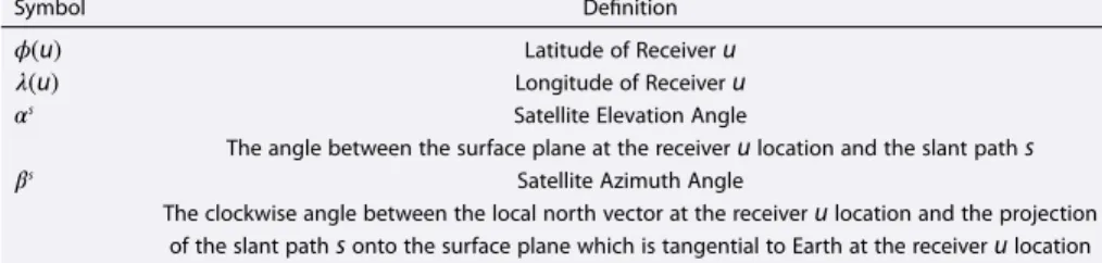
Figure 2. (a)𝜙(Ps i), (b)𝜆(P s i), and (c)cos −1 (𝛾si)with respect to elevation for input parameters𝜙(u) = 39.92
◦,𝜆(u) = 32.85◦,𝛼s= 28◦, and𝛽s= 126◦.
Suppose that ΔHiis the height step value used at height Hi. In order to find the electron density
contribu-tion at each height, the length of the slant path s within the height step ΔHi, which will be denoted as ΔH s
i,
should be calculated. For this purpose, the following trigonometric relation can be used: ΔHs i= ΔHi cos(𝛾s i) . (9)
Finally, IRI-Plas model-based STEC value along the slant path s, which will be denoted as STECs, can be
approximated by integrating the electron density contributions from each height along the slant path s as nonuniform Riemann sum:
STECs = I ∑ i=1 Ne(𝜙(Ps i), 𝜆(P s i), Hi)ΔH s i, (10) where Ne(𝜙(Ps i), 𝜆(P s
i), Hi) represents the electron density value obtained from IRI-Plas model for given
lat-itude𝜙(Ps
i), longitude𝜆(P s
i), and height Hi, and I is the length of array H. For illustrative purposes, Figure 2
shows the𝜙(Ps
i),𝜆(P
s
i), and cos
−1(𝛾s
i) dependence to the height, respectively, for a sample STEC calculation
for the set of input parameters𝜙(u) = 39.92◦,𝜆(u) = 32.85◦,𝛼s= 28◦, and𝛽s= 126◦.
In choosing the set of layers whose heights are denoted with vector H, the trade-off between the accuracy and efficiency of the computation is considered. A longer vector H with denser height levels will yield more precise results while increasing the computational time. A nonuniform separation of layers with denser height levels at higher electron density regions and sparse height levels at lower electron density regions provides acceptable results.
a)
b)
Figure 3. (a) Mean value of 1000 randomly generated vertical electron density profiles from IRI-Plas, for randomly selected positions
on Earth, for randomly selected dates between 1 January 2003 and 1 January 2013, and for random hours. (b) Mean value of the abso-lute values of the first-order derivatives of 1000 randomly generated vertical electron density profiles used in Figure 3a, with respect to height.
30 210 60 240 90 270 120 300 150 330 180 0
Satellite Azimuth Angle
90 70
50 30
10
Satellite Elevation Angle
10:00 11:00 12:00 13:00 14:00 15:00 16:00 100 30 210 60 240 90 270 120 300 150 330 180 0
Satellite Azimuth Angle
90 70
50 30
10
Satellite Elevation Angle
13:00 14:00 15:00 16:00 17:00 18:00 19:00 30 210 60 240 90 270 120 300 150 330 180 0
Satellite Azimuth Angle
90 70
50 30
10
Satellite Elevation Angle
09:00 10:00 11:00 12:00 13:00 14:00
a)
b)
c)
d)
e)
f)
6 7 8 9 10 11 12 13 14 15 16 0 50 100 150 200 Hour (GMT) STEC (TECU) (12−Mar−2010) IONOLAB−STEC (12−Mar−2010) IRI−Plas based STEC (13−Apr−2012) IONOLAB−STEC (13−Apr−2012) IRI−Plas based STEC9 10 11 12 13 14 15 16 17 18 19 0 10 20 30 40 50 60 70 80 90 100 Hour (GMT) STEC (TECU) (12−Mar−2010) IONOLAB−STEC (12−Mar−2010) IRI−Plas based STEC (13−Apr−2012) IONOLAB−STEC (13−Apr−2012) IRI−Plas based STEC
5 6 7 8 9 10 11 12 13 14 0 10 20 30 40 50 60 Hour (GMT) STEC (TECU) (12−Mar−2010) IONOLAB−STEC (12−Mar−2010) IRI−Plas based STEC (13−Apr−2012) IONOLAB−STEC (13−Apr−2012) IRI−Plas based STEC
Figure 4. Comparison of IRI-Plas-STEC and IONOLAB-STEC values with respect to hour for 12 March 2010 (quiet day) and 13 April 2012
(geomagnetically disturbed day): (a) ntus, PRN 16; (c) ankr, PRN 7; and (e) kir0, PRN 20. Satellite tracks in local polar coordinate system for (b) PRN 16, (d) PRN 7, and (f ) PRN 20.
In order to investigate the proper selection of H, 1000 different vertical electron density distribution func-tions are generated by using IRI-Plas, for randomly selected posifunc-tions on Earth and for randomly selected dates between 1 January 2003 and 1 January 2013 and for random hours of the day. Figure 3a shows the mean value of the obtained electron density distributions, and Figure 3b shows the mean value of the absolute values of the first-order derivatives of the obtained electron density distributions, with respect to height. The regions with higher first-order derivative require denser allocation of the layers. The maximum value of the first-order derivative is reached at the height of 236 km. At a height of 600 km, this value drops below 8% of the maximum value. At 1300 km height and above, IRI-Plas model employs plasmasphere
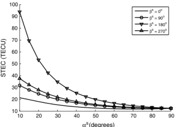
10 20 30 40 50 60 70 80 90 10 20 30 40 50 60 70 80 90 100 αs (degrees) STEC (TECU) βs = 0o βs = 90o βs = 180o βs = 270o
Figure 5. IRI-Plas-based STEC calculations with respect to satellite elevation angle parameter on 22 April 2009 at 12:00 GMT for a receiver
station located at coordinates (39◦N, 35◦E) and for a GPS satellite position located at north, east, west, and south of the receiver station.
equations, and the first-order derivative drops below 0.8% of its maximum value. Consequently, use of 1 km height step sizes between 100 and 600 km, 10 km step sizes between 600 and 1300 km, and 50 km step sizes between 1300 and 20,000 km has been found to provide acceptable computational results.
2.1. STEC With Respect to Hour of the Day
By using the proposed methodology, real STEC measurements obtained from GPS systems can be directly compared with the IRI-Plas model-based STEC estimates. For this purpose, IONOLAB-STEC data is used as experimental GPS measurement [Nayir et al., 2007]. Figure 4 shows a comparison of IRI-Plas-STEC calcula-tions and GPS-based STEC measurements (IONOLAB-STEC data) with respect to hour. Two different days are selected for calculations: 12 March 2010, which is a quiet day, and 13 April 2012, which is a geomagnet-ically disturbed day. IONOLAB-STEC and IRI-Plas-STEC values are computed for three different GPS receiver stations located at equatorial, mid and high latitude regions. The equatorial station “ntus” is located at Sin-gapore, Republic of SinSin-gapore, the mid latitude station “ankr” is located at Ankara, Turkey, and the high latitude station ‘kir0’ is located at Kiruna, Sweden. Receiver location and satellite angles for each hour, which are required to calculate IRI-Plas-STEC values, are obtained from IONOLAB-STEC computations. For each sta-tion, a satellite that passes close to local zenith angle is chosen. These satellites are PRN 16 for ntus, PRN 7 for ankr and PRN 20 for kir0. Figure 4 indicates that the computations of STEC from IRI-Plas and IONOLAB-STEC are in agreement with each other for a quiet day, yet they may differ significantly on a geomagnetically dis-turbed day. This is mainly due to the fact that IRI-Plas Ne profiles are based on Consultative Committee on International Radio (CCIR) monthly median coefficients.
2.2. STEC With Respect to Satellite Elevation Angle
In order to see the effect of satellite elevation angle in the STEC estimation, STEC values are calculated for synthetic satellite positions which have constant satellite azimuth angles and a range of satellite elevation angles in the interval [10◦, 90◦] with a step size of 10◦. Figure 5 shows STEC values obtained on 22 April
2009, 12:00 Greenwich Mean Time (GMT), for a receiver station located at coordinates (39◦N, 35◦E). Four
dif-ferent satellite azimuth angles are used in calculations: 0◦(north), 90◦(east), 180◦(south), and 270◦(west).
Note that STEC values converge to the same vertical TEC value as the satellite elevation angle increases. As the satellite elevation decrease, STEC estimates show variation based on the electron density distribu-tion at the corresponding azimuth direcdistribu-tions. Figure 5 indicates higher electron density values in the south and lower electron density values in the north. Typically, in GPS measurements, ionosphere is considered to be uniform and homogeneus for satellite elevation angles greater than 60◦. Calculating STEC values by sweeping a range of satellite elevation angles provides a means to investigate the validity of this commonly used assumption.
2.3. STEC With Respect to Satellite Azimuth Angle
Investigation of STEC with respect to satellite azimuth angles provide characteristics of anisotropy in the ionosphere. For this purpose, STEC values are calculated for synthetic satellite positions which have constant satellite elevation angles and a range of satellite azimuth angles in the interval [0◦, 350◦] with a step size
−180 −150 −120 −90 −60 −30 0 30 60 90 120 150 180 10 12 14 16 18 20 22 24 26 βs (degrees) STEC (TECU) αs = 40o αs = 60o αs = 80o
Figure 6. IRI-Plas-based STEC calculations with respect to satellite azimuth angle parameter on 22 April 2009 at 12:00 GMT for a receiver
station located at coordinates (39◦N, 35◦E) and for satellite elevation angles of 40◦, 60◦, and 80◦.
of 10◦. Figure 6 shows STEC values obtained on 22 April 2009, 12:00 GMT, for a receiver station located at
coordinates (39◦N, 35◦E). Three different satellite elevation angles are used in calculations: 40◦, 60◦, and 80◦.
The calculated STEC is minimum for azimuth angle of 10◦and maximum for azimuth angle of −170◦, which
indicates an increase in the electron density toward the south. Figure 6 also indicates the effect of satellite elevation angle on the STEC measurements. As the satellite elevation angle decreases, the effect of satellite azimuth angle on the STEC measurements gets stronger. This functionality also demonstrates the validity of azimuthal homogeneity assumptions with respect to satellite elevation angles.
3. Online STEC Calculation Service
In order to present an online, easy-to-use STEC calculation service, proposed STEC estimation approach is implemented as a public web-based service at www.ionolab.org. Users have to register to the website before using the IRI-Plas-STEC service. In order to use this service, users do not need to download any pro-gram or propro-gram code; all calculations are performed online by the IONOLAB service. For a given time, satellite, and receiver parameters, STEC values are calculated and presented to user online or via e-mail. For receiver parameters, user can input receiver coordinates or four-character IGS or EPN station code. For satellite parameters, user can input satellite elevation angle and azimuth angle values or just the GPS satel-lite number. IRI-Plas-STEC service is a unique application which accepts IGS or EPN station codes and GPS satellite numbers as slant path input parameters. This property simplifies the model-based estimations of STEC corresponding to real STEC measurement scenarios. Furthermore, optional services for calculating STEC by sweeping hour of the day, satellite elevation angle, and satellite azimuth angle parameters are also integrated to this service. Figure 7 shows a screenshot of the IRI-Plas-STEC service.
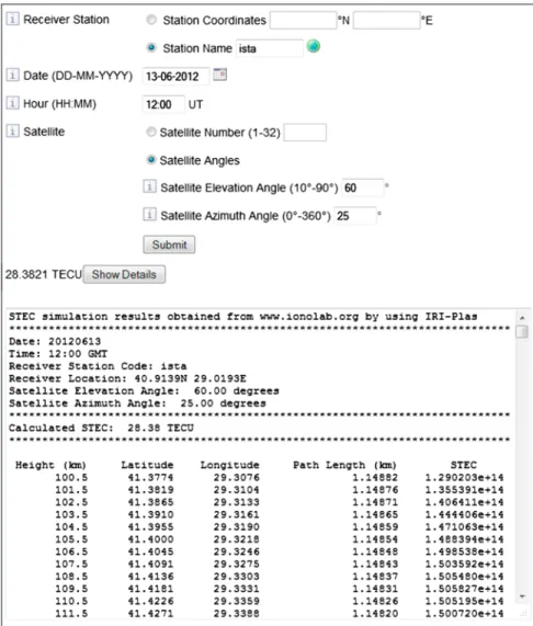
Figure 8. Screenshot of the computed single IRI-Plas-STEC value.
3.1. Single STEC Calculation
Single STEC calculation option is the default functionality provided by the IRI-Plas-STEC service. This option calculates a single STEC value for a given time, receiver, and satellite parameters. For receiver parameters, user can choose between specifying the coordinates of the receiver or entering the four-digit IGS or EPN sta-tion code. For satellite parameters, user can input satellite angles or a GPS satellite number. IONOLAB service collects information about the given receiver and satellites or uses given coordinate and angle parameters directly to calculate the requested STEC value. Results are presented to the user online, together with cal-culation details such as slant path parameters and electron density values on the slant path obtained from IRI-Plas. Calculation time for a single STEC takes a couple of minutes. Figure 8 shows the screenshot of a sam-ple single STEC calculation results. In this examsam-ple, receiver station is selected as “ista,” which is located in Istanbul, Turkey; calculation date is selected as 13 June 2012, 12:00 GMT; satellite elevation angle is selected as 60◦; and the satellite azimuth angle is selected as 25◦yielding an estimated result of 28.31 TECU.
Calcu-lation details such as the coordinates of the receiver station, coordinates of the slant path as the altitude reaches definite altitude values and the electron density values at these points, and the length of the slant path at each altitude step are also provided to the user.
3.2. STEC Calculation With Respect to Hour of the Day
In this option, user provides date, receiver, and satellite parameters in order to obtain hourly IRI-Plas-STEC values at a specified date. If the user specifies satellite angles, IRI-Plas-STEC values are calculated hourly for corresponding fixed slant path. However, if the user specifies the GPS satellite number, GPS satellite positions on the given date are obtained from satellite ephemerides data, and IRI-Plas-STEC values are
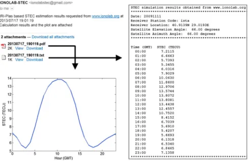
Figure 9. Screenshot of an e-mail sent by IRI-Plas-STEC service that contains requested STEC calculation results with respect to hour.
calculated hourly for a slant path that follows the satellite. Calculation time for this option takes about an hour; therefore, every calculation request is queued at the server, and when the calculations are completed, user is informed by an e-mail together with the detailed results and a plot of the obtained results. If the user enters the four-digit IGS or EPN station code and GPS satellite number, this option provides a very infor-mative tool for the comparison of GPS-based daily STEC measurements and IRI-Plas-based STEC estimates. Figure 9 shows a sample e-mail providing the obtained results. In this example, receiver station is selected as “ista,” which is located in Istanbul, Turkey. The calculation date is selected as 11 November 2009; satellite elevation angle and satellite azimuth angle are selected as 66◦. IRI-Plas-STEC service automatically retrieves
coordinates of the receiver station and calculates STEC values from 00:00 GMT to 23:00 GMT with hourly intervals on the specified date. Figure 9 shows that the calculated STEC values change between 5.34 TECU, which is obtained at 03:00 GMT, and 13.08 TECU, which is obtained at 11:00 GMT.
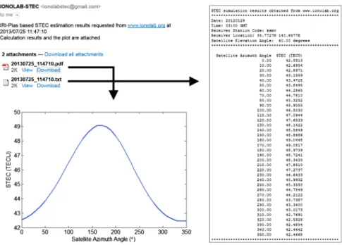
Figure 10. Screenshot of an e-mail sent by IRI-Plas-STEC service that contains requested STEC calculation results with respect to satellite
Figure 11. Screenshot of an e-mail sent by IRI-Plas-STEC service that contains requested STEC calculation results with respect to satellite
azimuth angle.
3.3. STEC Calculation With Respect to Satellite Elevation Angle
In this option, user provides date, receiver, and satellite azimuth angle parameters. User can specify the coordinates of the receiver or enter the four-digit IGS or EPN station code. STEC values are calculated for satellite elevation angle values between 10◦and 90◦with a step size of 10◦. Calculation time for this option
is about half an hour, which also depends on the overall calculation load on the IONOLAB server. Therefore, every calculation request is queued at the server, and when the calculations are finished, user is informed by an e-mail together with the detailed results and a plot. Figure 10 shows content of a sample e-mail. In this example, receiver station is selected as “ankr,” which is located in Ankara, Turkey. The calculation time is selected as 22 June 2010, 11:00 GMT, and the satellite azimuth angle is selected as 78◦. IRI-Plas-STEC service automatically retrieved coordinates of the receiver station and calculated STEC values for satellite elevation angle values ranging from 10◦to 90◦with a step size of 10◦. Figure 10 shows that the calculated STEC values
have a range between 16.48 TECU, which is obtained for 85◦satellite elevation angle, and 38 TECU, which is
obtained for 10◦satellite elevation angle.
3.4. STEC Calculation With Respect to Satellite Azimuth Angle
In this option, user specifies date, receiver, and satellite elevation angles. User can specify the coordinates of the receiver or enter the four-digit IGS or EPN station code. STEC values are calculated for satellite azimuth angle values between 0◦and 350◦with a step size of 10◦. Calculation time for this option is about an hour; therefore every calculation request is queued at the server, and when the calculations are finished, user is informed by an e-mail together with the detailed results and a plot. This option provides valuable informa-tion for analyzing the anisotropic characteristics of the ionosphere. Figure 11 shows content of a sample e-mail. In this example, receiver station is selected as “ksmv,” which is located in Kashima, Japan. The calcu-lation date is specified as 29 January 2009, 03:00 GMT, and the satellite elevation angle is selected as 60◦.
IRI-Plas-STEC service automatically retrieved coordinates of the receiver station and calculated STEC values for satellite azimuth angle values ranging from 0◦to 350◦with a step size of 10◦. Figure 11 shows that the calculated STEC values have a range between 42.44 TECU, which is obtained for 340◦satellite azimuth angle, and 49.08 TECU, which is obtained for 170◦satellite azimuth angle.
4. Conclusions
An efficient computational technique is proposed for the estimation of STEC from a given 3-D model of the ionosphere. IRI-Plas model, which is an extended version of IRI to the plasmasphere is used for the esti-mation of the climatic component of the 3-D electron density profile in the ionosphere. Proposed method
approximates required line integration with a nonuniform Riemann sum for precise calculation of STEC values from IRI-Plas model. A user-friendly web service based on the presented IRI-Plas-STEC calculation approach has been implemented at www.ionolab.org website, together with the calculation options such as STEC with respect to satellite elevation angle, satellite azimuth angle, and hour of the day parameters. The IRI-Plas-STEC values can be used in various studies for ionospheric research and recovery of GNSS ionospheric delay errors.
References
Arikan, F., C. B. Erol, and O. Arikan (2003), Regularized estimation of vertical total electron content from Global Positioning System data,
J. Geophys. Res., 108(A12), 1469, doi:10.1029/2002JA009605.
Arikan, F., H. Nayir, U. Sezen, and O. Arikan (2008), Estimation of single station interfrequency receiver bias using GPS-TEC, Radio Sci., 43, RS4004, doi:10.1029/2007RS003785.
Bilitza, D. (2001), International Reference Ionosphere 2000, Radio Sci., 36(2), 261–275.
Cabrera, M. A., R. G. Ezquer, and S. M. Radicella (2005), Predicted and measured slant ionospheric electron content, J. Atmos. Sol. Terr.
Phys., 67(16), 1566–1572.
Coïsson, P., S. M. Radicella, R. Leitinger, and B. Nava (2006), Topside electron density in IRI and NeQuick: Features and limitations, Adv.
Space Res., 37, 937–942.
Davies, K., and G. K. Hartmann (1997), Studying the ionosphere with the Global Positioning System, Radio Sci., 32(4), 1695–1703. Erturk, O., O. Arikan, and F. Arikan (2009), Tomographic reconstruction of the ionospheric electron density as a function of space and
time, Adv. Space Res., 43, 1702–1710.
EUREF Permanent Network (2013), http://www.epncb.oma.be/_networkdata/stationmaps.php.
Gulyaeva, T. L. (2010), Storm time behavior of topside scale height inferred from the ionosphere-plasmasphere model driven by the F2 layer peak and GPS-TEC observations, Adv. Space Res., 47(6), 913–920, doi:10.1016/j.asr.2010.10.025.
Gulyaeva, T. L., F. Arikan, and I. Stanislawska (2011), Inter-hemispheric imaging of the ionosphere with the upgraded IRI-Plas model during the space weather storms, Earth Planets Space, 63(8), 929–939, doi:10.5047/eps.2011.04.007.
Gulyaeva, T. L. (2012), Empirical model of ionospheric storm effects on theF2layer peak height associated with changes of peak electron density, J. Geophys. Res., 117, A02302, doi:10.1029/2011JA017158.
Gulyaeva, T. L., and D. Bilitza (2012), Towards ISO Standard Earth Ionosphere and Plasmasphere Model, in New Developments in the
Standard Model, edited by R. J. Larsen, pp. 1–39, Nova, Hauppauge, New York.
Gulyaeva, T. L., F. Arikan, M. Hernandez-Pajares, and I. Stanislawska (2013), GIM-TEC adaptive ionospheric weather assessment and forecast system, J. Atmos. Sol. Terr. Phys., 102, 329–340.
Hirooka, S., K. Hattori, M. Nishihashi, S. Kon, and T. Takeda (2012), Development of ionospheric tomography using Neural Network and its application to the 2007 Southern Sumatra earthquake, Electr. Eng. Jpn., 181(4), 9–18.
International GNSS Service (2013), http://igscb.jpl.nasa.gov/.
Jin, S., and R. Jin (2011), GPS Ionospheric Mapping and Tomography: A case of study in a geomagnetic storm, IEEE Geoscience and Remote
Sensing Symposium (IGARSS) 2011, 24–29 July 2011, Vancouver, Canada, 1127–1130.
Komjathy, A. (1997), Global ionospheric total electron content mapping using the global positioning system, PhD dissertation, Depart-ment of Geodesy and Geomatics Engineering Technical Report No.188, University of New Brunswick, Fredericton, New Brunswick, Canada, 248 pp.
Lanyi, G. E., and T. Roth (1988), A comparison of mapped and measured total ionospheric electron content using Global Positioning System and beacon satellite observations, Radio Sci., 23(4), 483–492.
Maltseva, O. A., G. A. Zhbankov, and N. S. Mozhaeva (2013), Advantages of the new model of IRI (IRI-Plas) to simulate the ionospheric electron density: Case of the European area, Adv. Radio Sci., 11, 307–311.
Manucci, A. J., B. D. Wilson, D. N. Yuan, C. H. Ho, U. J. Lindqwister, and T. F. Runge (1998), A global mapping technique for GPS-derived ionospheric total electron content measurements, Radio Sci., 33, 565–582.
Mushini, S. C., P. T. Jayachandran, R. B. Langley, and J. W. MacDougall (2009), Use of varying shell heights derived from ionosonde data in calculating vertical total electron content (TEC) using GPS—New method, Adv. Space Res., 44(11), 1309–1313.
Nava, B., P. Coïsson, and S. M. Radicella (2008), A new version of the NeQuick ionosphere electron density model, J. Atmos. Sol. Terr. Phys.,
70(15), 1856–1862.
Nayir, H., F. Arikan, O. Arikan, and C. B. Erol (2007), Total electron content estimation with Reg-Est, J. Geophys. Res., 112, A11313, doi:10.1029/2007JA012459.
Radicella, S. (2009), The NeQuick model genesis, uses and evolution, Ann. Geophys., 52(3-4), 417–422.
Schaer, S. (1999), Mapping and predicting the Earth’s ionosphere using the Global Positioning System, PhD thesis, Univ. of Bern, Bern, Switzerland.
Sibanda, P. (2010), Challenges in topside ionospheric modelling over South Africa, PhD dissertation, Rhodes University, South Africa.
Acknowledgments
This study is supported by grants from TUBITAK 109E055, joint TUBITAK 110E296 and RFBR 11-02-91370-CT_a, and joint TUBITAK 112E568 and RFBR 13-02-91370-CT_a.