LOCAL SIGNAL DECOMPOSITION BASED
METHODS FOR THE CALCULATION OF
THREE-DIMENSIONAL SCALAR OPTICAL
DIFFRACTION FIELD DUE TO A FIELD GIVEN ON
A CURVED SURFACE
a thesis
submitted to the department of electrical and
electronics engineering
and the graduate school of engineering and science
of b
˙Ilkent university
in partial fulfillment of the requirements
for the degree of
doctor of philosophy
By
Erdem S
¸ahin
I certify that I have read this thesis and that in my opinion it is fully adequate, in scope and in quality, as a thesis for the degree of Doctor of Philosophy.
Prof. Dr. Levent Onural (Supervisor)
I certify that I have read this thesis and that in my opinion it is fully adequate, in scope and in quality, as a thesis for the degree of Doctor of Philosophy.
Prof. Dr. Haldun M. ¨Ozakta¸s
I certify that I have read this thesis and that in my opinion it is fully adequate, in scope and in quality, as a thesis for the degree of Doctor of Philosophy.
Prof. Dr. A. Aydın Alatan
I certify that I have read this thesis and that in my opinion it is fully adequate, in scope and in quality, as a thesis for the degree of Doctor of Philosophy.
Assoc. Prof. Dr. Mehmet Tankut ¨Ozgen
I certify that I have read this thesis and that in my opinion it is fully adequate, in scope and in quality, as a thesis for the degree of Doctor of Philosophy.
Assoc. Prof. Dr. U˘gur G¨ud¨ukbay
Approved for the Graduate School of Engineering and Science:
Prof. Dr. Levent Onural
ABSTRACT
LOCAL SIGNAL DECOMPOSITION BASED
METHODS FOR THE CALCULATION OF
THREE-DIMENSIONAL SCALAR OPTICAL
DIFFRACTION FIELD DUE TO A FIELD GIVEN ON
A CURVED SURFACE
Erdem S
¸ahin
Ph.D. in Electrical and Electronics Engineering
Supervisor: Prof. Dr. Levent Onural
May 2013
A dimensional scene or object can be optically replicated via the three-dimensional imaging and display method holography. In computer-generated holography, the scalar diffraction field due to a field given on an object (curved surface) is calculated numerically. The source model approaches treat the build-ing elements of the object (such as points or planar polygons) independently to simplify the calculation of diffraction field. However, as a tradeoff, the accu-racies of fields calculated by such methods are degraded. On the other hand, field models provide exact field solutions but their computational complexities make their application impractical for meaningful sizes of surfaces. By using the practical setup of the integral imaging, we establish a space-frequency sig-nal decomposition based relation between the ray optics (more specifically the light field representation) and the scalar wave optics. Then, by employing the uncertainty principle inherent to this space-frequency decomposition, we derive
an upper bound for the joint spatial and angular (spectral) resolution of a phys-ically realizable light field representation. We mainly propose two methods for the problem of three-dimensional diffraction field calculation from fields given on curved surfaces. In the first approach, we apply linear space-frequency sig-nal decomposition methods to the two-dimensiosig-nal field given on the curved surface and decompose it into a sum of local elementary functions. Then, we write the diffraction field as a sum of local beams each of which corresponds to such an elementary function on the curved surface. By this way, we increase the accuracy provided by the source models while keeping the computational complexity at comparable levels. In the second approach, we firstly decompose the three-dimensional field into a sum of local beams, and then, we construct a linear system of equations where we form the system matrix by calculating the field patterns that the three-dimensional beams produce on the curved surface. We find the coefficients of the beams by solving the linear system of equations and thus specify the dimensional field. Since we use local beams in three-dimensional field decomposition, we end up with sparse system matrices. Hence, by taking advantage of this sparsity, we achieve considerable reduction in com-putational complexity and memory requirement compared to other field model approaches that use global signal decompositions. The local Gaussian beams used in both approaches actually correspond to physically realizable light rays. Indeed, the upper joint resolution bound that we derive is obtained by such Gaussian beams.
Keywords: Linear Space-Frequency Signal Decomposition, Gaussian Beam
De-composition, Curved Surfaces, Computer-Generated Holography, Scalar Optical Diffraction, Light Field Representation, Integral Imaging, Ray Optics, Scalar Wave Optics
¨
OZET
E ˘
GR˙I B˙IR Y ¨
UZEY ¨
UZER˙INDE VER˙ILEN ALANA KARS
¸ILIK
GELEN ¨
UC
¸ BOYUTLU SKALAR OPT˙IK ALANIN
HESAPLANMASI ˙IC
¸ ˙IN LOKAL S˙INYAL AYRIS
¸TIRMA
TABANLI Y ¨
ONTEMLER
Erdem S
¸ahin
Elektrik ve Elektronik M¨
uhendisligi B¨
ol¨
um¨
u Doktora
Tez Y¨
oneticisi: Prof. Dr. Levent Onural
Mayıs 2013
¨
U¸c boyutlu sahneler veya nesneler, bir ¨u¸c boyutlu g¨or¨unt¨uleme ve g¨osterim tekni˘gi olan holografi aracılı˘gıyla optik olarak yeniden ¨uretilebilir. Verilen bir cisim (e˘gri y¨uzey) tarafından olu¸sturulan kırınım deseni, klasik holografinin dı¸sında, bilgisayar ortamında sayısal olarak da hesaplanabilir. Kaynak model yakla¸sımları, kırınım deseninin hesaplanmasını kolayla¸stımak i¸cin nesnenin nokta veya d¨uzlemsel ¸cokgen gibi yapı ta¸slarını ba˘gımsız bir ¸sekilde ele alırlar. Ancak, bir ¨od¨unle¸sim olarak, bu y¨ontemler aracılı˘gıyla hesaplanan kırınım desenlerinin do˘grulukları azalır. Di˘ger taraftan, alan modelleri do˘gru alan ¸c¨oz¨umleri sunarlar fakat bu modellerin hesap karma¸sıklıkları anlamlı boyutlardaki y¨uzeylere uygu-lanamamalarına neden olur. T¨umlev g¨or¨unt¨uleme (integral imaging) y¨onteminin pratik d¨uzene˘gini kullanarak, ı¸sın opti˘gi (¨ozel olarak ı¸sık alanı g¨osterimi) ile skalar dalga opti˘gi arasında uzay-frekans sinyal ayrı¸stırma tabanlı bir ili¸ski kuruyoruz. Ardından, bu uzay-frekans ayrı¸stırma y¨onteminin do˘gasında var olan belirsizlik ilkesinden faydalanarak, fiziksel olarak ger¸ceklenebilir ı¸sık alanı g¨osterimi i¸cin bir birle¸sik uzamsal ve a¸cısal (spektral) ¨ust ¸c¨oz¨un¨url¨uk sınırı buluyoruz. E˘gri
y¨uzeylerden yayılan ¨u¸c boyutlu kırınım deseninin hesaplanması i¸cin esas olarak iki de˘gi¸sik y¨ontem sunuyoruz. Birinci yakla¸sımda, e˘gri y¨uzey ¨uzerinde verilen iki boyutlu alana do˘grusal uzay-frekans sinyal ayrı¸stırma y¨ontemlerini uyguluyor ve bu alanı lokal temel fonksiyonların toplamı olacak ¸sekilde b¨ol¨uyoruz. Ardından, kırınım desenini her biri e˘gri y¨uzey ¨uzerindeki bu temel fonksiyonlardan birine kar¸sılık gelen lokal ı¸sık h¨uzmelerinin toplamı ¸seklinde yazıyoruz. Bu sayede, kay-nak modelleri tarafından sa˘glanan alanın do˘gruluk de˘gerini, hesap karma¸sıklı˘gını onlarla kar¸sıla¸stırılabilir seviyede tutarak, artırıyoruz. ˙Ikinci yakla¸sımda, ilk olarak ¨u¸c boyutlu alanı lokal h¨uzmelerin toplamı olacak ¸sekilde b¨ol¨uyoruz. Ardından, bir do˘grusal denklemler sistemi olu¸sturuyoruz, ¨oyle ki bu sistemi temsil eden sistem matrisinin kolonlarını ¨u¸c boyutlu h¨uzmelerin e˘gri y¨uzey ¨
uzerinde ¨uretti˘gi alan desenlerini bularak elde ediyoruz. H¨uzmelerin katsayılarını do˘grusal denklemler sistemini ¸c¨ozerek buluyoruz. B¨oylece, ¨u¸c boyutlu alanı be-lirlemi¸s oluyoruz. U¸c boyutlu alanı ayrı¸stırırken lokal h¨¨ uzmeler kullandı˘gımız i¸cin seyrek sistem matrisleri elde ediyoruz. Bundan yararlanarak, global sinyal ayrı¸stırma y¨ontemi kullanan alan modellerine g¨ore hesaplama karma¸sıklı˘gı ve bellek ihtiyacını ¨onemli derecede azaltıyoruz. ˙Iki yakla¸sımda da kullanılan lokal Gauss h¨uzmeleri aslında fiziksel olarak ger¸ceklenebilir ı¸sınlara kar¸sılık gelmek-tedir. Buldu˘gumuz birle¸sik ¨ust ¸c¨oz¨un¨url¨uk sınırı da esasen bu Gauss h¨uzmeleri tarafından elde edilmektedir.
Anahtar Kelimeler: Do˘grusal Uzay-Frekans Sinyal Ayrı¸stırma, Gauss H¨uzme Ayrı¸stırma, E˘gri Y¨uzeyler, Bilgisayarla ¨Uretilmi¸s Holografi, Skalar Optik Kırınımı, I¸sık Alanı G¨osterimi, T¨umlev G¨or¨unt¨uleme, I¸sın Opti˘gi, Skalar Dalga Opti˘gi
ACKNOWLEDGMENTS
I would like to express my sincere thanks to my supervisor Prof. Dr. Levent Onural for his guidance, support and encouragement during every phase of this research.
I would also like to thank Prof. Dr. Haldun M. ¨Ozakta¸s, Prof. Dr. A. Aydın Alatan, Assoc. Prof. Dr. Mehmet Tankut ¨Ozgen and Assoc. Prof. Dr. U˘gur G¨ud¨ukbay for reading and commenting on the thesis.
This work is partially supported by European Commission within FP6 under Grant 511568 with acronym 3DTV.
I acknowledge the financial support of T ¨UB˙ITAK (The Scientific and Technolog-ical Research Council of Turkey) between 2006-2011.
I also acknowledge the financial support of Bilkent University between 2011-2013. I would like to thank Erdem Ulusoy (who is like a brother to me) for everything. Finally, I want to express my deepest gratitude to my family for their uncondi-tional and unfailing support. I dedicate this dissertation to them.
Contents
1 Introduction 1
1.2 Holography . . . 4 1.3 The Scalar Wave Optics and Diffraction Theory . . . 6
1.4 Organization of the Dissertation . . . 12
2 The Relation of Light Field Representation to Integral Imaging
and Scalar Wave Optics 13
2.1 Light Field Representation . . . 14
2.2 Integral Imaging . . . 17
2.3 Relation of Light Field Representation to Integral Imaging . . . . 18 2.4 The Spatio-Angular Resolution Tradeoff in the Light Field
Rep-resentation . . . 21
3 Calculation of the 3D Scalar Diffraction Field from the Field Given on a Curved Surface by Using Linear and Local Signal
Decomposition Methods 28
3.1.1 Continuous Decomposition for Planar Input Surfaces . . . 31
3.1.2 Discrete Decomposition for Planar Input Surfaces . . . 32
3.2 Curved Input Surfaces . . . 36
3.2.1 Continuous Decomposition for Curved Input Surfaces . . . 37
3.2.2 Discrete Decomposition for Curved Input Surfaces . . . 39
3.3 Short Time Fourier Transform . . . 41
3.3.1 STFT for Planar Input Surfaces . . . 41
3.3.2 STFT for Curved Input Surfaces . . . 44
3.4 Wavelet Decomposition . . . 46
3.4.1 Wavelet Decomposition for Planar Input Surfaces . . . 46
3.4.2 Wavelet Decomposition for Curved Input Surfaces . . . 49
4 Calculation of the 3D Scalar Diffraction Field from the Field Given on a Curved Surface via Gaussian Signal Decomposition 54 4.1 Gaussian Signal Decomposition . . . 56
4.1.1 Decomposition for the Planar Input Surface Case . . . 56
4.1.2 Decomposition for the Curved Input Surface Case . . . 61
4.2 Simulation Results . . . 66
5 Calculation of the 3D Scalar Diffraction Field from the Field Given on a Curved Surface via 3D Gaussian Beam
5.1 Diffraction Field Calculation from the Fields Given on Planar In-put Surfaces . . . 83 5.2 Diffraction Field Calculation from the Fields Given on Curved
Input Surfaces . . . 85 5.3 Simulation Results . . . 90
List of Figures
2.1 The relation of solid angle, dΩ, to the differential area, dA2.
( c⃝2010 The Imaging Science Journal. Reprinted with permis-sion. Published in [40]). . . 15
2.2 Representation of the ray power density in the discrete case. ( c⃝2010 The Imaging Science Journal. Reprinted with permis-sion. Published in [40]) . . . 16
2.3 Parameterization of the light power density in integral imaging. ( c⃝2010 The Imaging Science Journal. Reprinted with permission. Published in [40]) . . . 20
3.1 Local coordinate system on the input curved surface. ( c⃝2012 JOSA A. Reprinted with permission. Published in [35]) . . . 37
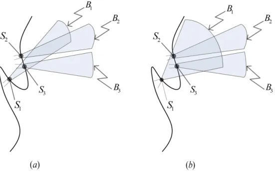
4.1 Mutual couplings between patches on a curved surface (2D cross sections of the surface and beams are shown for the sake of sim-plicity). (a) Mutual coupling between S1 and S3 patches, (b)
mutual coupling between S1 and S2 patches (in addition to the
mutual coupling between S1 and S3 patches). ( c⃝2012 JOSA A.
4.2 The 2D simulation setup which is periodic along the x-axis (the fields used in the simulations repeat themselves between each dashed horizontal lines shown in the figure). ( c⃝2012 JOSA A. Reprinted with permission. Published in [35]) . . . 67
4.3 The discrete Gaussian synthesis window function gd[n] =
exp ( −L2 s σ2n2 )
for σ = 2.20µm and Ls = 0.26µm. ( c⃝2012 JOSA
A. Reprinted with permission. Published in [35]) . . . 70 4.4 The discrete analysis window function corresponding to the
Gaus-sian synthesis window function gd[n] = exp
( −L2 s σ2n2 ) , for σ = 2.20µm and Ls = 0.26µm, for the case that the shift parameters
in space and frequency are M = 16 and K = 32, respectively. ( c⃝2012 JOSA A. Reprinted with permission. Published in [35]) . 71
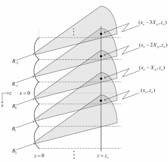
4.5 Periodic Gaussian beams induced by the periodic pattern over the periodic curved line. ( c⃝2012 JOSA A. Reprinted with permission. Published in [35]) . . . 73
4.6 The real part of the discrete input signal, ud[n], on the circular
arc with a measure of 30 degrees (imaginary part is zero). ( c⃝2012 JOSA A. Reprinted with permission. Published in [35]) . . . 75
4.7 The magnitude of the 2D diffraction field due to the input signal ˜
ud[n], one period of which is shown in Fig. 4.6, on the circular arc
with a measure of 30 degrees. ( c⃝2012 JOSA A. Reprinted with permission. Published in [35]) . . . 76 4.8 The magnitude of the 2D diffraction field due to a single shifted
and modulated Gaussian window function, with parameters m = 16 and k = 1, on the circular arc with a measure of 30 degrees. ( c⃝2012 JOSA A. Reprinted with permission. Published in [35]) . 77
4.9 The real parts of the original, ud[n], and reconstructed, urd[n],
signals on the circular arc with a measure of 30 degrees. ( c⃝2012 JOSA A. Reprinted with permission. Published in [35]) . . . 80
5.1 The setup of the proposed Gaussian beam decomposition method (a 2D pattern is shown for the sake of simplicity). ( c⃝2013 JOSA A. Reprinted with permission. Published in [81]) . . . 87
5.2 The periodic 2D simulation setup. ( c⃝2013 JOSA A. Reprinted with permission. Published in [81]) . . . 94
5.3 The ratios of the complexities of the operations QRPWD, SQR-PWD, QRGBD to the complexity of SQRGBD (note that the result shown for SQRGBD is “1”). ( c⃝2013 JOSA A. Reprinted with permission. Published in [81]) . . . 96
5.4 The sparsity of the system matrices for the proposed Gaussian beam decomposition method. ( c⃝2013 JOSA A. Reprinted with permission. Published in [81]) . . . 97
5.5 The absolute value of the system matrix G which has size 2400× 2000 and formed by the application of the proposed Gaus-sian beam decomposition method to the curved line shown in Fig. 5.2. ( c⃝2013 JOSA A. Reprinted with permission. Published in [81]) . . . 98
5.6 The real part of the system matrix G which has size 2400× 2000 and formed by the application of the plane wave decomposition method to the curved line shown in Fig. 5.2. (note that the absolute values of all matrix entries are one.) Note the difference with respect to Fig. 5.5 in terms of sparsity. ( c⃝2013 JOSA A. Reprinted with permission. Published in [81]) . . . 99
5.7 One period of the two-dimensional (x, z) field corresponding to the signal given on the periodic curved line which has loops. . . . 101 5.8 The absolute value of the system matrix G which has size 1400×
986 and formed by the application of the proposed Gaussian beam decomposition where the beam waist positions are chosen inside the loops. . . 102
5.9 The absolute value of the system matrix G which has size 1400× 986 and formed by the application of the proposed Gaussian beam decomposition where the beam waist positions are chosen on the curved line. . . 103 5.10 One period of the two-dimensional (x, z) field corresponding to the
Gaussian beam decomposition where the beam waist positions are taken inside the loops and all the beam coefficients are taken equal.104 5.11 The real part of the system matrix G which has size 1400× 1000
and formed by the application of the plane wave decomposition method for the curved line shown in Fig. 5.7. Note that the absolute values of all matrix entries are one. . . 105
5.12 One period of the 2D periodic curved surface. ( c⃝2013 JOSA A. Reprinted with permission. Published in [81]) . . . 107 5.13 One period of the 2D periodic object. (Gilles Tran c⃝2007
www.oyonale.com, used under the Creative Commons Attribution license. Published in [81] ) . . . 108
5.14 The absolute value of the system matrix G which has size 11664×9472 and formed by the application of the proposed Gaus-sian beam decomposition method for the curved surface given in Fig. 5.12. Note that the figure is enhanced for better visualiza-tion. ( c⃝2013 JOSA A. Reprinted with permission. Published in [81]) . . . 109
5.15 The real part of the system matrix G which has size 11664× 9475 and formed by the application of the plane wave decomposition method for the curved surface given in Fig. 5.12. Note that the absolute values of all matrix entries are one. Note also that the random noise-like appearance is a consequence of the structure of the surface given in Fig. 5.12. ( c⃝2013 JOSA A. Reprinted with permission. Published in [81]) . . . 110 5.16 The absolute value of the system matrix G which has size
3973× 2809 and formed by the application of the proposed Gaus-sian beam decomposition method for the object given in Fig. 5.13. ( c⃝2013 JOSA A. Reprinted with permission. Published in [81]) . 111
5.17 The real part of the system matrix G which has size 3973× 2819 and formed by the application of the plane wave decomposition method for the object given in Fig. 5.13. Note that the absolute values of all matrix entries are one. ( c⃝2013 JOSA A. Reprinted with permission. Published in [81]) . . . 112
List of Publications
This dissertation is based on the following publications.
[Publication-I] E. S¸ahin and L. Onural, “A comparative study of light field representation and integral imaging,” The Imaging Science Journal, vol. 58, no. 1, pp. 28-31, 2010.
[Publication-II] E. S¸ahin and L. Onural, “Scalar diffraction field calculation from curved surfaces via Gaussian beam decomposition,” J. Opt. Soc. Am. A, vol. 29, no. 7, pp. 1459-1469, 2012.
[Publication-III] E. S¸ahin and L. Onural, “Calculation of the scalar diffraction field from curved surfaces by decomposing the 3D field into a sum of Gaussian beams,” J. Opt. Soc. Am. A, vol. 30, no. 3, pp. 527-536, 2013.
The contributions of the author to the publications which are listed above were as follows: In Publications-I, -II and -III, the author designed and im-plemented the proposed algorithms and methods, performed the mathematical derivations and prepared the manuscripts. The author conducted and reported the simulations in Publications-II and -III.
Chapter 1
Introduction
Nowadays, the three-dimensional (3D) media applications become more and more popular as a consequence of successfully produced 3D films and games. In such media applications, usually the stereoscopic viewing and display techniques are used. Although the stereoscopy is actually the simplest 3D visualization tech-nique and were discovered many years ago, it seems to be sufficient to attract people, at least for now. During the capturing stage of stereoscopy, the 3D con-tent is obtained by using two cameras placed side by side [1, 2]. Then in the display stage, the image captured by the right (left) camera is presented to the right (left) eye of the observer [3]. Although the stereoscopic images are dis-played on the same screen, each eye of the observer perceives different images by wearing goggles such as polarized glasses or active shutter glasses. The neces-sity of wearing goggles is one of the main drawbacks of the stereoscopic viewing techniques. In this sense, the autostereoscopic viewing seems to be an attractive alternative to stereoscopy. The autostereoscopy provides 3D viewing without imposing a necessity of wearing goggles [4]. The well known autostereoscopic imaging technique, integral imaging, was discovered by Lippmann at 1908 [5]. Several display devices that provide autostereoscopic views have been produced since then, but nowadays the producers have begun to advertise autostereoscopic
displays more seriously hoping them to be the next generation 3D visualization technique.
Holography provides the richest optical content among other viewing tech-niques for a given 3D scene. Indeed, the term hologram originates from the Greek words holos and gramma that mean “whole” and “message”, respectively. Ideally, holography aims to capture a 3D scene by a holographic imaging method and replicate the 3D scene at some other place by an appropriate holographic display device. In classical holography, the optical information related to a 3D scene is captured on a recording device (hologram) by using a reference beam [6, 7]. The interference of the optical wave due to the 3D scene (diffraction field) and the reference beam produce the coded optical information of the 3D scene. This coding is actually an amplitude modulation of the diffraction field by the reference wave as in the communication systems [8]. The 3D scene is replicated by illuminating the hologram with the same reference beam as used in the recording stage.
The recording stage of classical holography makes it unpractical for 3D video applications. With the invention of charged coupled devices (CCD), however, it became possible to record dynamic images. As a consequence of that, the interest of optics community to digital holography gained momentum [9]. The digital holography is different from the classical optical holography in the sense that in digital holography the images of a 3D scene is captured by a CCD camera instead of recording it on a photographic film. A further development in the holography was gained with the inclusion of computers in the process of hologram calculation. In this so-called computer-generated holography (CGH) process, the holograms of desired 3D fields are calculated numerically by computation [10, 11, 12]. On the other hand, the invention of dynamically programmable spatial light modulator (SLM) devices made it also possible to display 3D dynamic images [3]. All these
developments have led the research projects related to end-to-end holographic 3D television systems [3, 13, 14].
As mentioned before, capturing and displaying a 3D content are two main operations in holography. Although usually planar sensor and display devices are used for these operations, several advantages of curved display and sensor devices have been recently reported. For example, spherical geometries are shown to be more useful compared to planar ones to reduce the resolution requirements of the sensor and display devices [15, 16]. In the work of Hahn et al. [17], curved array of spatial light modulators (SLMs) is used as a holographic display device to increase the field of view compared to conventional planar array of SLMs. Similar possible advantages of curved display and sensor devices for holography indicate the need for the theoretical analysis of diffraction between curved surfaces. On the other hand, calculation of the diffraction field due to an object is one of the main tasks to be accomplished in computer-generated holography. The challenging part of this task is to provide an approach which is both computationally efficient and satisfactorily accurate, since it is generally a computationally costly process to calculate the 3D diffraction field due to an object. As addressed by these discussions, the methods that we propose in this dissertation provide effective and efficient ways to calculate the 3D diffraction field due to an object or due to a two-dimensional (2D) field given on a curved surface.
In the remaining part of this chapter, we give more detailed information about holography. We also discuss the scalar wave optics and the diffraction theory of light, since we adopt the scalar diffraction theory in the methods that we develop for the problem of diffraction field calculation due to a 2D field given on a curved surface.
1.2
Holography
Holography was invented by D. Gabor in 1947, while he was researching a method to improve the resolution of an electron microscope [18]. The development of holograms started, however, in 1960’s with the invention of truly coherent light source laser by the scientist C. Towns, A. Prokhorov and N. Bassov [19]. In 1962, the first laser transmission type hologram of a 3D objet was obtained by E. Leith and J. Upatnieks. The hologram was needed to be illuminated by a laser in order to produce 3D images with realistic depth and clarity. In the same year, N. Denisyuk developed white-light reflection type hologram. It is possible to view such type of holograms under incandescent lighting. Transmission type of white-light holography was invented by S. A. Benton in 1968. White-light transmission type of holograms can be viewed in ordinary white light. Dynamic 3D images were obtained in 1972 with the development of integral hologram method by L. Cross [20]. Integral holography combines white-light transmission holography with the cinematography to produce dynamic 3D images. The first computer-generated hologram was introduced in 1965 by B. R. Brown and A. W. Lohmann [21].
The computer-generated holography makes it possible to produce the holo-grams of objects (which may be synthetically generated) via numerical methods. That is an important improvement over the classical optical holography. How-ever, as mentioned before, the computational complexity of the diffraction field calculation is the main drawback of CGH. Significant developments have been achieved towards the aim of reducing the computation time since the introduc-tion of first computer-generated hologram [9, 11]. The Fresnel approximaintroduc-tion has been a widely used approach to reduce the computation time of digital holo-grams [8, 22]. In the Fresnel model, the propagation kernel is a 2D separable function. Furthermore, the wave propagation calculation which is modeled by the Fresnel integral can be implemented by the Fourier transform techniques.
The underlying purpose in the development of holographic stereograms [23, 24] is also to reduce the computation time. In the holographic stereogram approach, the hologram plane is partitioned into segments. The 2D complex function to be written inside a segment is determined according to the relative position of the center point of that segment with respect to the object. Thus, the computation time is reduced, since the field is not calculated for each pixel in the segment. Another widely used assumption in CGH is to model the object as a collection of point sources or planar polygons [23, 25, 26, 27, 28, 29, 30]. In these source model approaches, as is the case in other simplifications, there is a tradeoff be-tween the accuracy of the calculated field and the computational complexity. In Chapter 3 and Chapter 4 of this dissertation, we present an approach that in-creases the accuracy compared to such source model approaches by keeping the computational complexity at comparable levels.
The mathematical derivations related to holography are obtained by using the interference theory [31]. If we denote the reference wave as Ur and the
diffraction field due to the object as Uo, then the intensity of the field captured
on the hologram plane (interference pattern) is written as
I =|Uo+ Ur|2 . (1.1)
The expression given by Eq. 1.1 can be expanded as
I =|Uo|2+|Ur|2+ Uo∗Ur+ UoUr∗ , (1.2)
where ∗ is the complex conjugation operator. The interference pattern can be captured by a photographic film (transparency) or by a CCD camera. On the other hand, in the computer-generated holography, the diffraction field Uo due to
the given object is calculated numerically. Afterwards, the interference pattern can be calculated as given by Eq. 1.1. The reconstruction of the object wave is achieved via the diffraction of the same reference wave by the hologram recorded on the transparency. The field just after the transparency is written as
The object wave Uo appears as the fourth term (+1 order term) of Eq. 1.3.
The first two terms (zero order terms) represent the modulation of the reference wave by the intensities of the object and reference waves, respectively. The third term (−1 order term) is the modulated conjugate object wave. If these terms are separated in space, then the reconstructed object can be seen clearly. Under the assumption that the object wave is angle-limited, such a separation can be achieved by using an off-axis system where the reference and object waves are offset (there is a small angle between the reference and object waves). The min-imum offset angle requirement for an off-axis holographic system can be relieved by taking the intensity of the reference wave much larger than that of the object wave and thus making the first term of Eq. 1.3 negligible [31].
1.3
The Scalar Wave Optics and Diffraction
Theory
There are basically four models developed to describe the nature of light. These are ray optics, scalar wave optics (or simply wave optics), electromagnetic op-tics and quantum opop-tics. The simplest model ray opop-tics defines the light as a collection of rays which travel according to the Fermat’s principle [31]. The ray optics can adequately explain many optical phenomena such as reflection and refraction. In the ray optics (geometric optics), it is possible to assign different values to the rays which intersect at a given point and travel towards different directions. This property is not valid according to the diffraction phenomena which is explained by the wave optics. Similarly, the interference phenomenon of light can not be explained by the ray optics. The scalar wave optics encompasses the ray optics such that the ray optics can be seen as the limit of the wave op-tics when the wavelength of the light gets infinitesimally small [31]. The optical phenomena such as diffraction and interference are explained by the wave nature
of the light. On the other hand, there are situations like the diffraction of light at high angles or the interaction of light with a dielectric media where the scalar wave optics is not adequate. For such cases vector-valued descriptions of the light field are necessary. At this point, the electromagnetic optics provides sufficient descriptions. In electromagnetic optics, the propagation of light is modeled by using two mutually coupled vector waves, an electric field wave and a magnetic field wave. In free space, these fields satisfy the well-known Maxwell’s equations. The electromagnetic optics is not sufficient to describe the optical phenomena which are quantum mechanical in nature [31]. Such phenomena can be explained by the quantum optics.
In this dissertation, as mentioned before, we mainly deal with the problem of diffraction field calculation due to a 2D field given on a curved surface that is one of the challenging tasks in holography. In the methods proposed in Chapter 3, Chapter 4 and Chapter 5, we adopt the scalar wave optics and use linear space-frequency signal decompositions. At this point, it is important to note that there is a close relation between the local space-frequency decomposition of a scalar wave field and its ray optics approximation. The construction of a rigorous mathematical relation of the ray optics to the scalar wave optics based on the space-frequency uncertainty is another problem that we deal in this dissertation. The study related to this problem is given in Chapter 2. Here, it is worth noting that the construction of such a relation helped us to consider the approaches proposed in the subsequent chapters from the ray optics point of view.
In scalar wave optics, the light is assumed to propagate in the form of waves. An optical wave is described via a real-valued scalar function ut(x, t) of position
x = [x, y, z]T ∈ R3 and time t ∈ R3. A given optical wave satisfies the wave equation given by [8, 32], ∇2u t− 1 c2 ∂2u t ∂t2 = 0 , (1.4)
where c denotes the speed of light in free space and ∇2 = ∂2 ∂x2 + ∂
2
∂y2 + ∂ 2
As is most often the case in holography, we deal with monochromatic waves in this dissertation. The scalar wave function of a monochromatic wave is written in the form of [31],
ut(x, t) = a(x)cos{2πνt + ϕ(x)} , (1.5)
where a(x), ϕ(x) and ν represent the amplitude, phase and frequency (in cy-cles/unit time) of the monochromatic wave, respectively. For a purely monochro-matic wave, it is possible to omit the time dependence and use the phasor repre-sentation of the wave function, since the phasor reprerepre-sentation itself adequately describes the light. The phasor representation (complex amplitude) of the wave function is defined as
u(x) = a(x) exp{jϕ(x)} , (1.6)
where ut(x, t) = R {u(x) exp(j2πνt)}. If we substitute the complex amplitude
into the wave equation, we end up with the Helmholtz equation given as (
∇2+ 4π2
λ2
)
u = 0 , (1.7)
where λ is the wavelength of the monochromatic wave and c = λν.
Note that we will use the phasor representation of the wave field from now on. The entire field in 3D space can be specified by defining a 2D field on an infinite extent planar surface. Let the input field is specified on the z = 0 plane and defined as u0(x, y) = u(x, y, 0). According to the scalar diffraction theory,
the diffraction field on another plane which is parallel to z = 0 plane and placed at a distance z is given by [8, 33, 34],
uz(x, y) = u0(x, y)∗ ∗hz(x, y) , (1.8)
where ∗∗ denotes the two-dimensional convolution and hz(x, y) is the free space
propagation kernel. The exact field relation (under the scalar wave optics) be-tween such two parallel planes is given by the Rayleigh-Sommerfeld (RS) integral
which is obtained when the RS kernel hz(x, y) =− z 2π√x2+ y2+ z2 ( 1− jk√x2+ y2+ z2 ) exp(jk√x2+ y2+ z2) x2+ y2+ z2 (1.9) is substituted into the equation
uz(x, y) = ∞ ∫ −∞ ∞ ∫ −∞ u0(ξ, η)hz(x− ξ, y − η)dξdη . (1.10)
Denoting the Fourier transforms of u0(x, y), uz(x, y) and hz(x, y) as U0(fx, fy),
Uz(fx, fy) and Hz(fx, fy), respectively, Eq. 1.10 can be written in the frequency
domain as
Uz(fx, fy) = U0(fx, fy)Hz(fx, fy) , (1.11)
where, for the RS model, Hz(fx, fy) is given as [8, 34],
Hz(fx, fy) = F {hz(x, y)} = exp ( j2π λ z √ 1− (λfx)2− (λfy)2 ) . (1.12)
Here note that the Fourier transform from the (x, y) domain to the (fx, fy)
do-main, of a 2D function a(x, y) is defined as
A(fx, fy) = ∞ ∫ −∞ ∞ ∫ −∞
a(x, y) exp{−j2π(fxx + fyy)}dxdy . (1.13)
Now, as it can be proved by Eq. 1.11 that the plane waves, which are defined as exp(j2πfxTx
)
where x = [x, y, z]T and f
x = [fx, fy, fz]T, are actually the
eigenfunctions of the scalar diffraction (note that the scalar diffraction is actu-ally a linear shift invariant system). Therefore, the diffraction field at x that corresponds the 2D field specified on z = 0 plane can be also written as
u(x) = ∞ ∫ −∞ ∞ ∫ −∞ A(fx, fy) exp{j2π(fxTx)}dfxdfy , (1.14)
where fx2 + fy2 + fz2 = λ12 and λ is the wavelength of the plane waves. The coefficient of each plane wave is found by using the field u0(x, y) specified on the
reference input plane at z = 0 as A(fx, fy) = ∞ ∫ −∞ ∞ ∫ −∞ u0(x, y) exp{−j2π(fxx + fyy)}dxdy . (1.15)
The expression given by Eq. 1.14 is known as the plane wave decomposition. In this dissertation, we take into account only the propagating plane waves whose frequency components along the x and y axes satisfy fx2+fy2 ≤ λ12. In other words, we exclude the evanescent waves. The propagating plane waves occupy the 2D circular spatial frequency band which has a radius 1λ. For the case that the evanescent waves are ignored, the plane wave decomposition is written as
u(x) = ∫∫ B A(fx, fy) exp ( j2πfxTx ) dfxdfy , (1.16)
where B denotes the 2D frequency band occupied by the propagating plane waves [35]. The propagation kernel and transfer function that correspond to this case are given, respectively, as [8],
hz(x, y) = z jλ exp ( j2πλ√x2+ y2+ z2 ) x2 + y2+ z2 , (1.17) Hz(fx, fy) = exp ( j2πzλ√1− (λfx)2− (λfy)2 ) , for √f2 x + fy2 ≤ 1 λ 0, otherwise . (1.18) In Eq. 1.16, a monochromatic 3D field is written as a sum of infinite extent plane waves propagating toward different directions defined by the vector fx.
The plane wave decomposition given by Eq. 1.16 together with the analysis equation given by Eq. 1.15, uniquely determines the 3D field corresponding to a 2D field specified on the infinite extent reference plane at z = 0, provided that the propagation direction components of the plane waves along the z-axis is always positive (or they are all negative). Note that such a requirement is necessary, since, for example, the two plane waves given by exp{j2π(fxx + fyy + fzz)} and
on the z = 0 plane and thus they can not be discriminated from this 2D pattern. Therefore, in this dissertation, we also assume that a given 3D field u(x) :R3 → C is formed by a superposition of propagating plane waves with fz > 0.
If the plane wave components of the input field which is specified on the
z = 0 plane make small angles with the z-axis, i.e. fx2 + fy2 ≪ λ12, then the corresponding wave is called as paraxial wave. For the propagation of paraxial waves, the RS impulse response function can be approximated with a quadratic phase exponential function as
hz(x, y) = exp(j2πλz) jλz exp { jπ λz(x 2+ y2) } . (1.19)
This impulse response function is called as the Fresnel kernel and the diffraction model resulting from application of the Fresnel kernel is known as the Fresnel approximation [31].
The diffraction models such as Rayleigh-Sommerfeld, plane wave decompo-sition and Fresnel give the field relation (under the scalar diffraction theory) between the fields over two parallel planes. For the case that the input field is specified on a curved surface, direct application of formulations related to these models produce inconsistent 3D field solutions [36]. On the other hand, for such cases, the plane wave decomposition is also employed in a field model approach in the work of Esmer et al. [36, 37] and as a result an exact method is achieved. However, there are drawbacks of that approach such as intolerable computational complexity and memory requirement for large size of surfaces. At this point the local signal decomposition method that we propose in Chapter 5 plays a crucial role, in the problem of diffraction field calculation due to a field given on a curved surface, by decreasing both the computation time and memory requirement with respect to the approach introduced in [36], by still providing exact solutions.
1.4
Organization of the Dissertation
The work presented in this dissertation can be categorized into two parts. In the first part, we develop a mathematical relation between the ray optics and the scalar wave optics. More specifically, we firstly relate the light field representation (which is a ray optics based modeling of light) to the integral imaging. Then, by using the integral imaging as a bridge between the ray optics and wave optic, we develop a space-frequency decomposition based relation between the ray optics and the scalar wave optics. As a consequence of the uncertainty principle inherent to this space-frequency decomposition, we also derive an upper bound for the joint spatial and angular (spectral) resolution of a physically realizable light field representation. This part constitutes the second chapter of the dissertation. In the second part (Chapters 3-5), we deal with the problem of the calculation of 3D diffraction field from a 2D field given on a curved surface. In Chapter 3, we develop a generic local signal decomposition framework for the solution of this problem. As a special case of this framework, a Gaussian signal decomposition method is introduced in Chapter 4, where we provide explicit 3D field solutions and related simulations. In the methods proposed in Chapter 3 and Chapter 4, the field given on a 2D curved surface is mainly decomposed into a sum of local elementary signals. Then, the 3D field is written as a sum of local 3D beams each of which corresponds to such an elementary signal. In Chapter 5, we introduce another approach which is based on a 3D Gaussian beam decomposition method. In this method, the problem is formulated as a system of linear equations where the columns of the system matrix are the field patterns that the Gaussian beams produce on the curved surface. Thus, we solve a linear system of equations in order to find the 3D field due to a 2D field given on a curved surface.
Chapter 2
The Relation of Light Field
Representation to Integral
Imaging and Scalar Wave Optics
Light field representation is a three-dimensional image representation method that models the light as a collection of rays [38]. In other words, the ray optics model of light is adopted in the light field representation. The ray optics produces sufficiently accurate results when the light propagates around the objects having much greater dimensions compared to the wavelength of the light. Thus, as mentioned in Chapter 1, it can be viewed as the limit of the scalar wave optics as the wavelength of the light is infinitesimally small [31]. Beyond this observation, we construct a mathematical relation between the ray optics based model light field representation and scalar wave optics in this chapter. The mathematical relation is based on the space-frequency decomposition of the scalar wave field. The 3D optical imaging and display method integral imaging provides a natural way for this decomposition. The physical nature of lenses used in the integral imaging setup together with the diffraction phenomena explains the uncertainty
regarding the spatio-angular resolution tradeoff in the light field representation [39].
In Sec. 2.1 and Sec. 2.2, we introduce the light field representation and in-tegral imaging methods, respectively. Then, we construct an equivalence relation between these two 3D image representation methods in Sec. 2.3. Based on the results obtained in Sec. 2.3, we relate the scalar wave optics to the ray optics (actually the light field representation) and develop an uncertainty relation re-garding the spatio-angular resolution tradeoff in the light field representation in Sec. 2.4. Note that most of the content of the work presented in Sec. 2.1, Sec. 2.2 and Sec. 2.3 of this chapter is published in [40].
2.1
Light Field Representation
The appearance of the world at any time from any given point through any given direction can be represented with the so called plenoptic (plenty of optic) func-tion, P (x, y, z, θ, ϕ, λ, t) [41]. In other words, the plenoptic function corresponds to the radiance associated with the light ray, at time t, with wavelength λ, that passes from a 3D point (x, y, z) towards the direction (θ, ϕ). In order to ease the notation, we will omit the variation with respect to t and λ. With further as-sumption of free space propagation and by keeping the viewing positions outside the convex hull of the scene one can also reduce the dimension of the plenoptic function to four since the radiance associated with the light ray along its path will be constant in this case [38]. The four dimensional plenoptic function is called as light field [38].
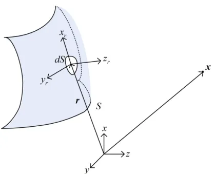
The light field is an abstract representation of the optical power flow associ-ated with the light rays. Let us define the infinitesimal power emanating from the differential surface dA1 (on an arbitrary surface W1) and reaching to the
Figure 2.1: The relation of solid angle, dΩ, to the differential area, dA2. ( c⃝2010
The Imaging Science Journal. Reprinted with permission. Published in [40]).
then associate a power density (for the power flow between W1 and W2 surfaces)
to the ray crossing the two surfaces at (x1, y1) and (x2, y2) and define it as
L(x1, y1, x2, y2) =
dP dA1dA2
. (2.1)
We call L(x1, y1, x2, y2) as the light field which can also be called ray power
density by taking into account physical quantities into consideration [40].
Instead of using the second surface and the differential area dA2 on it, it is
quite common to adopt a solid angle model in the literature [41, 42], and the density in that case is called the radiance. However, we prefer the definition given by Eq. 2.1 for our purposes. Incidentally, it is straightforward to establish the relation between the density given in Eq. 2.1 and the radiance by first noting that the differential solid angle is related to the differential area dA2 as
dΩ = dA2cos α2/D2 where α2 is the angle between the ray and the outward
normal to the W2 surface at (x2, y2) and D is the distance between (x1, y1) and
(x2, y2) (see Fig. 2.1). The radiance associated with the ray crossing the two
surfaces at (x1, y1) and (x2, y2) then becomes
˜
L(x1, y1, x2, y2) =
dP dA1cos α1dΩ
Figure 2.2: Representation of the ray power density in the discrete case. ( c⃝2010 The Imaging Science Journal. Reprinted with permission. Published in [40]) where dP is the radiant power emanating from dA1 and propagating along the
cone represented by the solid angle dΩ, dA1cos α1 is the projected differential
area on W1 along the direction of the ray and dΩ is the solid angle subtended by
dA2. Therefore, L and ˜L are closely related to each other with a normalization
as [40],
L(x1, y1, x2, y2) =
˜
L(x1, y1, x2, y2)
D2 cos α1cos α2 . (2.3)
Here note that the units of measurement of ˜L(x1, y1, x2, y2) and L(x1, y1, x2, y2)
are W m−2sr−1 and W m−4, respectively, where W (Watt) and sr (steradian) are the units of measurement of P and Ω, respectively.
Discretization of L(x1, y1, x2, y2) is necessary for digital processing. Instead
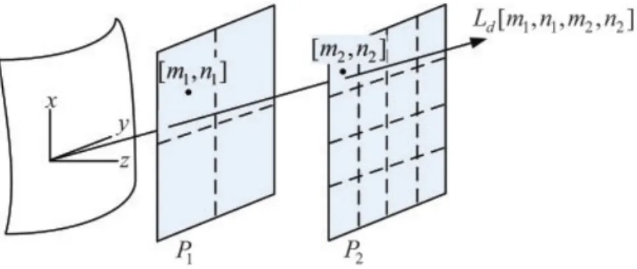
of arbitrary surfaces, we assume the simple two-parallel plane model [38, 43] where the P1 and P2 planes are usually defined as the camera and image planes
at z = z1 and z = z2, respectively. Let us assume that the index arrays [m1, n1]
and [m2, n2] represent the locations (m1M1, n1N1, z1) and (m2M2, n2N2, z2) on
the two parallel planes, respectively, where M1, N1, M2 and N2 are the sampling
intervals. Therefore [m1, n1] represents the centers of cameras (ideal pinhole
camera model), and [m2, n2] represents the sample points of the images that are
taken by the cameras. We define the discrete power density of the ray crossing the P1 and P2 planes, following the definition given by Eq. 2.1, as [40],
Ld[m1, n1, m2, n2] =
P [m1, n1, m2, n2]
S1S2
where S1 and S2 are the areas of the pixels on the P1 and P2 planes, respectively,
P [m1, n1, m2, n2] is the total power emanating from the pixel represented by
[m1, n1] and reaching to the pixel represented by [m2, n2]. (See Fig. 2.2)
There-fore, Ld represents the power flow between the two pixels [m1, n1] and [m2, n2]
on P1 and P2, respectively. The subscript d denotes that the field is discrete.
2.2
Integral Imaging
Integral imaging is a 3D image capture and display method. The image is cap-tured on a two-dimensional sensor array by a two-dimensional microlens array where the sensor array is placed behind the microlens array in a parallel fashion. Each microlens takes its own image of the 3D scene. The image that is formed behind each microlens is called as an elemental image. If the captured data is displayed properly, autostereoscopic images (allows 3D viewing without wearing eyeglasses) of 3D scenes are provided [5]. The parameterization of integral imag-ing is similar to the two-plane parameterization of the light field representation where the first plane P1 is the 2D microlens array plane and the second plane
P2 is the 2D sensor array plane (see Fig. 2.3). The display stage of an integral
imaging setup is constructed by placing the microlens array (used in the imaging stage) in front of the two-dimensional display device which displays the elemen-tal images captured by the two-dimensional sensor array. The integral imaging renders a pseudoscopic 3D reconstruction to the observer. There are several ways to convert the pseudoscopic images to orthoscopic ones [44].
The quality of the 3D image that a practical integral imaging setup provides depends on the physical properties of the lenslet and sensor arrays [45]. For example, it is possible to increase the viewing angle by placing the microlenses and sensors on curved surfaces [46]. The aperture size of the microlenses used for imaging is one of the main factors that determines the resolution, the depth
of field and the viewing angle of the 3D images provided by an integral imaging setup. The tradeoffs related to these quality factors are actually the consequences of the spatio-angular resolution tradeoff inherent to integral imaging and they are explained by the physical nature of the lenses and the scalar diffraction phenomena. Indeed, as will be shown in the following sections, this spatio-angular tradeoff makes the integral imaging play a bridging role in the aim of relating the ray optics to the scalar wave optics.
2.3
Relation of Light Field Representation to
Integral Imaging
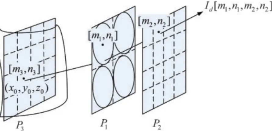
The counterpart of two parallel planes of light field representation in integral imaging is the microlens array plane P1 and the sensor array plane P2. However,
the P2 plane can be easily replaced by its image P3 which is a hypothetical plane
intersecting the 3D object volume (see Fig. 2.3). It is assumed that the captured elemental images are all in focus; by the way, this is necessary for a successful result in integral imaging. We will include both (P1, P2) and (P1, P3) plane pairs
in the discussion.
Let the light field between P3 and P1 planes be parameterized via the discrete
light field representation Ld[m3, n3, m1, n1]. Let the [m1, n1] array represent the
locations of the microlenses where the aperture of each microlens corresponds to a pixel on the P1 plane. Following the definition given by Eq. 2.4, one can find
the power density of the light emanating from (x0, y0, z0) on the object surface
and crossing the P3 plane at [m3, n3] and reaching the microlens at [m1, n1] as
ˆ
Id[m3, n3, m1, n1] =
P [m3, n3, m1, n1]
S1S3
, (2.5)
where S3is the area of a pixel on P3, S1is the area of the aperture of the microlens
and reaching the aperture of the microlens at [m1, n1] [40]. We used the notation
ˆ
I to represent the power flow between points on P3 and P1 planes; I is reserved
for power density between P1 and P2 planes; similar notation is adopted for L
and ˆL.
We place P3plane at z3 and adjust the locations of P1 and P2 planes such that
P2 and P3 planes become images of each other due to microlenses. Therefore,
according to the lens magnification equation
z1− z3 z2− z1 = ( S3 S2 )1 2 , (2.6)
where z1, z2 and z3 are again the z-coordinates of the P1, P2 and P3 planes,
respectively, and S2 is the area of the pixel [m2, n2] which is the image of the
pixel [m3, n3] (see Fig. 2.3).
Since the light power reaching the microlens [m1, n1] from an object point
(x0, y0, z0) via the pixel [m3, n3] on P3flows to the point [m2, n2] on P2 unchanged
(lossless lenses), where [m2, n2] is the image of [m3, n3], by using Eq. 2.5, we can
write that ˆ
Id[m3, n3, m1, n1]S1S3 = P [m3, n3, m1, n1]
= Id[m1, n1, m2, n2]S1S2 . (2.7)
Hence we can write that ˆ Id[m3, n3, m1, n1] = Id[m1, n1, m2, n2] ( S2 S3 ) , (2.8)
and this is consistent, as expected, with lens magnification between the P2 and
P3 planes [40]. Together with Eq. 2.8, the two equations
ˆ
Ld[m3, n3, m1, n1] = Iˆd[m3, n3, m1, n1] ,
Ld[m1, n1, m2, n2] = Id[m1, n1, m2, n2] (2.9)
establish the desired equivalence either between (P1, P3) plane pairs or (P1, P2)
Figure 2.3: Parameterization of the light power density in integral imaging. ( c⃝2010 The Imaging Science Journal. Reprinted with permission. Published in [40])
The integral imaging can be represented as a discrete light field either between
P3 and P1 or between P1 and P2 plane pairs, as given by Eq. 2.9, provided that
the depth of focus of the microlenses is large enough to focus any point on the 3D object into a pixel on P2 plane. Please note that this equivalence is valid under
the assumption that there is no cross-talk between the elemental images from different microlenses. In other words, we restrict the set of light frustum within a finite propagation angle behind each microlens such that overlaps are prevented [40]. This can simply be achieved by partitioning the sensor array plane to non-overlapping regions such that each partition corresponds to the elemental image of a particular microlens and the leakage from a microlens to the elemental image of any other microlens is prevented [47].
In order to relate the integral imaging to the light field representation in the continuous case, we need infinitely many infinitesimal microlenses on the infinite extent P1, and infinitely many infinitesimal sensors on the infinite extent P2
plane. Let us assume that the microlenses still possess the properties of an ideal lens even when their aperture sizes tend to zero. Even in this case, elimination of the cross-talk is practically impossible, since each elemental image size will also be infinitesimally small. Hence, the integral imaging cannot provide an equivalent representation to the continuous light field representation [40].
In all previous discussions, we assumed that microlenses provide a sufficient angular resolution for our purposes. Physically, a microlens having an infinitesi-mal aperture size behaves like a point light source and diffracts the incoming ray in an equally weighted manner to all angles. Therefore, our ability to assign an arbitrary propagation angle distribution is lost. This practical issue is a direct consequence of the uncertainty principle which states that we can not achieve ar-bitrary resolutions in both spatial and spectral (angular) domains of a signal [48]. Thus, the representation of the ray power densities with arbitrary resolutions in both spatial and angular domains is impossible via the light field representa-tion. In Sec. 2.4, we develop a rigorous mathematical relation regarding this spatio-angular resolution tradeoff in the light field representation.
2.4
The Spatio-Angular Resolution Tradeoff in
the Light Field Representation
As stated in Sec. 2.3, due to physical constraints we can not assign arbitrary values to the rays, which are defined by a point and a direction, since an in-finitesimal point emits the light in an equally weighted manner to all directions. Thus, an equality between the light field representation and the integral imaging is possible, if the microlenses have finite size apertures. Such an equality is devel-oped for the discrete case in Sec. 2.3. In this section, we investigate the integral imaging by using the scalar wave optics [45]. By this way, we are able to see the spatio-angular resolution tradeoff in the light field representation. Note that the link established between the light field representation and integral imaging in Sec. 2.3 leads us towards such an aim.
Firstly, let us write the effect of a thin lens (with focal length f ) on a wave field as [8],
uf(x, y) = u(x, y)pl(x, y) exp(jϕc) exp
{ −jπ λf(x 2 + y2) } , (2.10)
where u(x, y) is the wave field incident on the lens plane, pl(x, y) is the lens
aperture function which is defined as 1 inside the lens aperture and 0 outside of it; uf(x, y) is the wave field just after the lens. Note that exp(jϕc) is a constant
phase factor which is determined by the thickness of the lens. We will neglect this constant phase factor in the following discussions. Now let us assume that the lens plane is placed at z = 0. Then, the wave field at a distance z can be found as [8], u(x, y, z) = exp (j2π λ z ) jλz ∞ ∫ −∞ ∞ ∫ −∞ u0(ξ, η)pl(ξ, η) exp { −jπ λf(ξ 2 + η2) } exp { jπ λz [ (x− ξ)2 + (y− η)2]}dξdη , (2.11)
where u0(x, y) = u(x, y, 0). Note that here we employ the paraxial approximation
to ease the mathematical analysis. If we move the terms independent of ξ and η to out of the integral and rewrite the equation for the back focal plane at z = f , we end up with u(x, y, f ) = ϕ(x, y, f ) ∞ ∫ −∞ ∞ ∫ −∞ u0(ξ, η)pl(ξ, η) exp { −j2π λf (xξ + yη) } dξdη , (2.12) where ϕ(x, y, f ) = 1 jλf exp ( j2π λ f ) exp { jπ λf(x 2+ y2) } . (2.13)
The intensity of the field at (x, y) on the back focal is found as
I(x, y) =|u(x, y, f)|2 = Φ ∞ ∫ −∞ ∞ ∫ −∞ u0(ξ, η)pl(ξ, η) exp { −j2π λf (xξ + yη) } dξdη 2 , (2.14)
where
Φ = ϕ(x, y, f )ϕ∗(x, y, f ) = 1
λ2f2 (2.15)
is constant on the back focal plane. If we substitute fx = λfx and fy = λfy into
Eq. 2.14 as I(fxλf, fyλf ) = Φ ∞ ∫ −∞ ∞ ∫ −∞ u0(ξ, η)pl(ξ, η) exp{−j2π(fxξ + fyη)}dξdη 2 , (2.16) we see that the complex amplitude of the wave field at point (x, y, f ) is actu-ally determined by the Fourier component of the wave field u(x, y, 0) (which is incident on the lens plane) at frequencies (fx, fy) [8]. (See Eq. 1.13) The 2D
Fourier component at frequencies (fx, fy) is actually produced by the plane wave
exp{j2π(fxx + fyy + fzz)} where fx2 + fy2 + fz2 = λ12. Noting that the propa-gation direction of the plane wave exp{j2π(fxx + fyy + fzz)} is given by the
vector [fx, fy, fz]T, we can say that each 2D Fourier component on the z = 0
plane actually corresponds to a propagation direction. Therefore, in the follow-ing discussions we will use the frequency and angle interchangeably, for the sake of clarity.
Now, in order to extend the formulations to the integral imaging setup let us parameterize the power which is emanated from the microlens at the dis-crete point [m1, n1], on the microlens array plane, and propagates towards the
point (x, y) on the back focal plane as Lo(m1M1, n1N1, fx, fy) = I(fxλf, fyλf ).
Here, M1 and N1 are the distances between the consecutive microlenses along
the x and y axes, respectively. Please note that a similar expression to
Lo(m1M1, n1N1, fx, fy) is defined as the observable light field in [39]. We keep the
same definition and therefore use the subscript o to refer to an observable light field. The observability comes from the ability to assign an angular variation to the light emitted from a finite size aperture. By using the observable light field
integral imaging setup as Lo(m1M1, n1N1, fx, fy) = Φ ∞ ∫ −∞ ∞ ∫ −∞ u0(ξ, η)pl(ξ− m1M1, η− n1N1) exp{−j2π(fxξ + fyη)}dξdη 2 . (2.17) Thus, Lo(m1M1, n1N1, fx, fy) is actually the magnitude squared of the Fourier
transform of the windowed scalar wave field (apart from a constant) which is inci-dent on the microlens array plane. In other words, the power which is emanated from a lens on the microlens array plane and propagates towards a point on the back focal plane (can be viewed as the sensor array plane) is given as the magni-tude squared of the short time Fourier transform of the wave field incident on the microlens array plane, where the window function is the lens aperture function
pl(x, y). Note that the magnitude squared of short time Fourier transform is
called as the spectrogram. The spatio-angular resolution tradeoff in the observ-able light field is thus a direct consequence of the uncertainty principle inherent to spectrogram or STFT. In order to see that, let us rewrite Eq. 2.17 by using the Fourier transforms U0(fx, fy), Pl(fx, fy) of u0(x, y), pl(x, y), respectively, as
[49], Lo(m1M1, n1N1, fx, fy) = Φ ∞ ∫ −∞ ∞ ∫ −∞ U0(µ, ν)Pl(fx− µ, fy − ν) exp{j2π(m1M1µ + n1N1ν)}dµdν 2 . (2.18) The spatial resolution of the light field representation Lo(m1M1, n1N1, fx, fy) is
determined by the extent of the lens aperture function pl(x, y) as given by Eq.
2.17. On the other hand, the angular resolution is determined by the extent of the Fourier transform Pl(fx, fy) of the lens transfer function as given by Eq. 2.18.
Ac-cording to the uncertainty principle, both pl(x, y) and Pl(fx, fy) can not be made
and angle (frequency) of the light field representation Lo(m1M1, n1N1, fx, fy) can
not be obtained simultaneously. If we decrease the size of the aperture function, we achieve finer spatial resolution and as a tradeoff the angular (spectral) reso-lution is degraded, and vice versa. Thus, the spatio-angular resoreso-lution tradeoff in the light field representation Lo(m1M1, n1N1, fx, fy) is actually characterized
by the aperture function pl(x, y). Note that we developed the formulations in
this section by using the Fourier transform properties of the lenses. Although, we dealt with the intensity of the wave field at the back focal plane, the Fourier transform property of the lenses can be observed in any plane where the source is imaged [8].
The extent of the uncertainty related to the spatial and angular resolutions of the light field representation is given by the uncertainty principle. Before developing a mathematical expression about this uncertainty, let us give some definitions. The effective width ∆x of a 2D signal a(x, y) along the x-axis can be defined as [50], ∆x = ∞ ∫ −∞ ∞ ∫ −∞
(x− x0)2|a(x, y)|2dxdy
∞ ∫ −∞ ∞ ∫ −∞|a(x, y)| 2dxdy 1/2 , (2.19)
where x0 (the center of a(x, y) along the x-axis) is defined by
x0 = ∞ ∫ −∞ ∞ ∫ −∞
x|a(x, y)|2dxdy
∞ ∫ −∞ ∞ ∫ −∞|a(x, y)| 2dxdy . (2.20)
The effective width ∆y of a(x, y) along the y-axis and effective widths ∆fx, ∆fy
of the Fourier transform of a(x, y) along the fx and fy axes, respectively, are
defined similarly. For a 2D signal a(x, y) which has effective widths ∆x, ∆y in space and effective widths ∆fx, ∆fy in frequency, as defined by Eq. 2.19, one
form of the uncertainty principle states that [39, 50, 51] ∆x∆y∆fx∆fy ≥
1
By taking a(x, y) = pl(x, y) and denoting the effective widths of pl(x, y) along the
x and y axes as ∆x and ∆y, respectively, and the effective widths of Pl(fx, fy)
along the fx and fy axes as ∆fx and ∆fy, respectively, we can say that as a
consequence of the uncertainty principle given by Eq. 2.21, the effective areas of pl(x, y) and Pl(fx, fy) cannot be simultaneously made arbitrarily small. Here,
we assume that ∆x∆y and ∆fx∆fy give the effective areas occupied by pl(x, y)
and Pl(fx, fy), respectively [50]. We define the spatial and angular (spectral)
res-olutions of the (observable) light field representation Lo(m1M1, n1N1, fx, fy) as
1/(∆x∆y) and 1/(∆fx∆fy), respectively. Therefore, according to Eq. 2.21,
there is a restriction on the joint spatial and angular (spectral) resolution 1/(∆x∆y∆fx∆fy) of Lo(m1M1, n1N1, fx, fy) and indeed the joint resolution has
the upper bound 16π2 when the unit of frequencies are in cycles per unit length.
We call the light field representations which satisfy this joint resolution require-ment as physically realizable light field representations to refer to fields which are valid under the scalar wave optics. Here, it is once more worth noting that the 2D Fourier component of the light field Lo(m1M1, n1N1, fx, fy) at frequencies
(fx, fy) is produced by the plane wave exp{j2π(fxx + fyy + fzz)} whose
prop-agation direction is specified by the vector [fx, fy, fz]T. Therefore, we used the
frequency and angle interchangeably, for the sake of simplicity. The uncertainty principle derived by using the frequency variables can be actually applied to other scenarios where the light field is defined in a different form. For example, for the observable light field which is defined by using the slope variables u = x/z and v = y/z [39], the upper joint resolution bound 1/(∆x∆y∆u∆v) becomes 16π2/λ2 which can be simply found by a coordinate transformation between the
frequency and the slope variables, as noted in [39].
In this chapter, we constructed a mathematical relation between the ray optics (light field representation) and scalar wave optics. As a consequence of this relation, we provided an upper bound for the joint spatial and angular (spectral) resolutions of a physically realizable light field representation. In the subsequent


![Figure 4.3: The discrete Gaussian synthesis window function g d [n] = exp](https://thumb-eu.123doks.com/thumbv2/9libnet/5863646.120614/87.892.225.736.332.823/figure-discrete-gaussian-synthesis-window-function-g-exp.webp)
![Figure 4.4: The discrete analysis window function corresponding to the Gaussian synthesis window function g d [n] = exp](https://thumb-eu.123doks.com/thumbv2/9libnet/5863646.120614/88.892.222.736.309.815/figure-discrete-analysis-function-corresponding-gaussian-synthesis-function.webp)
![Figure 4.6: The real part of the discrete input signal, u d [n], on the circular arc with a measure of 30 degrees (imaginary part is zero)](https://thumb-eu.123doks.com/thumbv2/9libnet/5863646.120614/92.892.224.736.338.828/figure-discrete-input-signal-circular-measure-degrees-imaginary.webp)
