Behavioral/Cognitive
Functional Subdomains within Scene-Selective Cortex:
Parahippocampal Place Area, Retrosplenial Complex, and
Occipital Place Area
Tolga C
¸ukur,
1,2,3Alexander G. Huth,
5Shinji Nishimoto,
4and
X
Jack L. Gallant
5,6,71Department of Electrical and Electronics Engineering,2Ulusal Manyetik Rezonans Aras¸tırma Merkezi, Sabuncu Brain Research Center, and3Neuroscience Program, Bilkent University, Ankara 06800, Turkey,4Graduate School of Frontier Biosciences, Osaka University, Osaka 565-0871, Japan, and5Helen Wills Neuroscience Institute,6Program in Bioengineering, and7Department of Psychology, University of California, Berkeley, California 94720
Functional MRI studies suggest that at least three brain regions in human visual cortex—the parahippocampal place area (PPA),
retrosplenial complex (RSC), and occipital place area (OPA; often called the transverse occipital sulcus)—represent large-scale
informa-tion in natural scenes. Tuning of voxels within each region is often assumed to be funcinforma-tionally homogeneous. To test this assumpinforma-tion, we
recorded blood oxygenation level-dependent responses during passive viewing of complex natural movies. We then used a voxelwise
modeling framework to estimate voxelwise category tuning profiles within each scene-selective region. In all three regions, cluster
analysis of the voxelwise tuning profiles reveals two functional subdomains that differ primarily in their responses to animals, man-made
objects, social communication, and movement. Thus, the conventional functional definitions of the PPA, RSC, and OPA appear to be too
coarse. One attractive hypothesis is that this consistent functional subdivision of scene-selective regions is a reflection of an underlying
anatomical organization into two separate processing streams, one selectively biased toward static stimuli and one biased toward
dynamic stimuli.
Key words: category representation; fMRI; OPA; PPA; RSC; scene; subdomain; tuning profile; voxelwise model
Introduction
Visual scene perception is critical for our survival in the real
world. It is therefore reasonable to expect that the brain contains
neural circuitry specialized for processing the wealth of
informa-tion in natural scenes (
Field, 1987
;
Vinje and Gallant, 2000
;
Bar,
2004
;
Geisler, 2008
). At least three regions in the human brain—
the parahippocampal place area (PPA), the retrosplenial complex
(RSC), and the occipital place area (OPA)—produce larger blood
oxygenation level-dependent (BOLD) responses to scenes than to
isolated objects. These regions are therefore commonly
consid-ered to be involved in scene representation (
Grill-Spector and
Malach, 2004
;
Dilks et al., 2013
). The anatomical locations of
these regions are usually identified using functional localizers
(
Spiridon et al., 2006
). Each region of interest (ROI) is localized
by imposing a statistical threshold on the BOLD-response
con-Received Sept. 28, 2014; revised July 13, 2016; accepted July 28, 2016.
Author contributions: T.C¸., A.G.H., S.N., and J.L.G. designed research; T.C¸. performed research; T.C¸. and A.G.H. contributed unpublished reagents/analytic tools; T.C¸. analyzed data; T.C¸. and J.L.G. wrote the paper.
The work was supported in part by grants from the National Eye Institute (EY019684) and from the Center for Science of Information, an National Science Foundation Science and Technology Center, under Grant Agreement CCF-0939370. T.C¸.’s work was supported in part by a European Molecular Biology Organization Installation Grant (IG 3028), a Scientific and Technological Research Council of Turkey (TUBITAK) 2232 Fellowship (113C011), a Marie Curie Actions Career Integration Grant (PCIG13-GA-2013-618101), a TUBITAK 3501 Career Grant (114E546), and a Turkish Academy of Science Young Scientists Award Programme (TUBA-GEBIP) fellowship. We thank D. Stansbury, A. Vu, N. Bilenko, and J. Gao for their help in various aspects of this research.
The authors declare no competing financial interests.
Correspondence should be addressed to either of the following: Tolga C¸ukur, Department of Electrical and Elec-tronics Engineering, Bilkent University, Ankara TR-06800, Turkey. E-mail:[email protected]; or Jack L. Gal-lant, 3210 Tolman Hall #1650, University of California at Berkeley, Berkeley, CA 94720. E-mail:[email protected]
DOI:10.1523/JNEUROSCI.4033-14.2016
Copyright © 2016 the authors 0270-6474/16/3610257-17$15.00/0
Significance Statement
Visual scene perception is a critical ability to survive in the real world. It is therefore reasonable to assume that the human brain
contains neural circuitry selective for visual scenes. Here we show that responses in three scene-selective areas—identified in
previous studies— carry information about many object and action categories encountered in daily life. We identify two
subre-gions in each area: one that is selective for categories of man-made objects, and another that is selective for vehicles and
locomotion-related action categories that appear in dynamic scenes. This consistent functional subdivision may reflect an
ana-tomical organization into two processing streams, one biased toward static stimuli and one biased toward dynamic stimuli.
trast between scenes versus single objects. This localizer approach
implicitly assumes that all voxels within an ROI have similar
visual selectivity and that each ROI is functionally homogeneous
(
Friston et al., 2006
). However, recent reports suggest that
sub-regions within the PPA may differ in their visual responsiveness
(
Arcaro et al., 2009
), and that voxels within the PPA might have
heterogeneous spatial-frequency selectivity (
Rajimehr et al.,
2011
) and functional connectivity (
Baldassano et al., 2013
).
These findings suggest that the PPA, and perhaps other
scene-selective ROIs, might consist of several functional subdomains
that represent different visual information in natural scenes.
It is challenging to assess visual representations in
scene-selective areas because they are thought to respond to
higher-order correlations among natural image features that cannot be
easily decomposed (
Lescroart et al., 2015
). This difficulty has
fueled ongoing debates about what specific types of information
are represented in these areas (
Nasr et al., 2011
). Previous studies
suggested that scene-selective areas might represent low-level
in-formation related to spatial factors (
Epstein and Kanwisher,
1998
;
MacEvoy and Epstein, 2007
;
Park et al., 2007
,
2011
;
Kravitz
et al., 2011b
) and texture (
Cant and Goodale, 2011
), high-level
information related to scene categories (
Walther et al., 2009
;
Stansbury et al., 2013
), and/or contextual associations (
Bar et al.,
2008
). Some evidence also suggests that the PPA, RSC, and OPA
represent specific object categories (
Reddy and Kanwisher, 2007
;
Macevoy and Epstein, 2009
;
Mullally and Maguire, 2011
;
Troiani
et al., 2014
). A recent voxelwise modeling study from our
labo-ratory showed that some PPA voxels are selective for specific
categories of inanimate objects in natural scenes (
Huth et al.,
2012
). Furthermore, another voxelwise modeling study from our
laboratory showed that the fusiform face area (FFA), another
classical functional ROI that is also category-selective, consists of
several functional subdomains with diverse tuning properties
(
C¸ukur et al., 2013b
). Therefore, it is possible that scene-selective
areas might also comprise distinct functional subdomains with
different selectivity for object and action categories.
Here, we specifically assess the functional heterogeneity of
representations in the PPA, RSC, and OPA. We first recorded
BOLD signals evoked by a large set of natural movies. We then
used voxelwise modeling (
Huth et al., 2012
;
C¸ukur et al., 2013a
)
to determine how thousands of distinct object and action
catego-ries were represented in single voxels located within each of these
three ROIs. Finally, we performed cluster analysis on the
mea-sured category-tuning profiles to determine whether there are
functional subdomains with diverse tuning properties within
each ROI.
Materials and Methods
Subjects. Six healthy human subjects (S1–S6; mean age, 26.7⫾ 3.1 years;
five males; one female) with normal or corrected-to-normal vision par-ticipated in the study. The study consisted of five separate scan sessions: three sessions for the main experiment and two sessions for functional localizers. The protocols for these experiments were approved by the Committee for the Protection of Human Subjects at the University of California, Berkeley (UCB). Written informed consent was obtained from all subjects before scanning.
Main experiment. The main experiment was conducted in three
sepa-rate sessions. During each session, whole-brain BOLD responses were recorded while subjects passively viewed a distinct selection of color natural movies. Potential stimulus biases were minimized by selecting the movies from a diverse set of sources as described byNishimoto et al. (2011). High-definition movie frames were cropped to a square aspect ratio and down-sampled to 512⫻ 512 pixels (24 ⫻ 24°; the entire movie stimulus used as stimuli in this study is available athttp://crcns.org/
data-sets/vc/vim-2/about-vim-2). Subjects maintained steady fixation on a color dot (0.16⫻ 0.16°) superimposed onto the movies and located at the center of the visual field. The color of the dot changed at 3 Hz to ensure continuous visibility. Stimulus presentation was performed with an MRI-compatible projector (Avotec), a custom-built mirror system, and custom-designed presentation scripts.
Two separate datasets were acquired for training and testing voxelwise models. The training and test runs contained different natural movies, and the presentation order of these runs was interleaved during each scan session. A total of 12 training runs and 9 testing runs were acquired across the three sessions. A single training run lasted 10 min and was compiled by concatenating distinct 10 –20 s movie clips presented without repeti-tion. A single testing run was compiled by concatenating 10 separate 1 min blocks in random order. Each 1 min block was presented nine times across three sessions and evoked BOLD responses were averaged across these repeats. To minimize the effects of hemodynamic transients during movie onset, data collected during the initial 10 s of each run were dis-carded. These procedures resulted in a total of 3600 and 270 data samples for training and testing, respectively.
Note that these same data were analyzed in several recent studies from our laboratory (Huth et al., 2012; C¸ukuret al., 2013a,b).Huth et al. (2012)reported that category selectivity is organized in broad gradients distributed across the high-level visual cortex, and that some PPA voxels are selective for inanimate objects. However, that study did not system-atically examine the variability and spatial organization of tuning for nonscene categories within individual scene-selective ROIs. The work of
C¸ukur et al. (2013a)involved a study of selective attention with aims unrelated to those of the present study. In a separate study,C¸ukur et al. (2013b)discovered several functional subdomains within the FFA that showed differences in category tuning.
Functional localizers. Functional localizer data were acquired
indepen-dently from the main experiment. Localizers for category-selective brain areas consisted of six 4.5 min runs of 16 blocks. Each block lasted 16 s and contained 20 static images randomly selected from one of the following categories: objects, scenes, faces, body parts, animals, and spatially scrambled objects (Spiridon et al., 2006). The presentation order of the category blocks was randomly shuffled across runs. Within a block, each image was flashed for 300 ms, followed by a 500 ms blank period. To maintain vigilance, subjects were required to press a button when they detected two identical consecutive images. The localizer for retinotopi-cally organized early visual areas consisted of four 9 min runs containing clockwise rotating polar wedges, counter-clockwise rotating polar wedges, expanding rings, and contracting rings, respectively (Hansen et al., 2007). The localizer for the intraparietal sulcus consisted of one 10 min run of 30 blocks. Each block lasted 20 s and contained either a self-generated saccade task (among a pattern of targets) or a resting task (Connolly et al., 2000). The localizer for the human motion processing complex (MT⫹) consisted of four 90 s runs of 6 blocks. Each block lasted 15 s and contained either continuous or temporally scrambled natural movies (Tootell et al., 1995).
MRI parameters. Data collection was performed at UCB using a 3 T
Siemens Tim Trio MRI scanner (Siemens Medical Solutions) and a 32-channel receiver array.T2ⴱ-weighted functional data were collected using
a gradient-echo echo-planar imaging sequence with the following pa-rameters: TR⫽ 2 s; TE ⫽ 31 ms; a water-excitation pulse with flip angle of 70°; voxel size, 2.24⫻ 2.24 ⫻ 3.5 mm3; field-of-view, 224⫻ 224 mm2;
and 32 axial slices for whole-brain coverage. Anatomical data were col-lected using a T1-weighted magnetization-prepared rapid-acquisition gradient-echo sequence with the following parameters: TR⫽ 2.30 s, TE⫽ 3.45 ms, flip angle ⫽ 10°, voxel size ⫽ 1 ⫻ 1 ⫻ 1 mm2,
field-of-view⫽ 256 ⫻ 256 ⫻ 192 mm3.
Data preprocessing. Functional brain volumes acquired in individual
scan sessions were first motion-corrected and then aligned to the first session of the main experiment using Oxford Centre for Functional MRI of the Brain’s Linear Image Registration Tool (Jenkinson et al., 2002). For each run, the low-frequency drifts in BOLD responses of individual vox-els were removed using a median filter over a 120 s temporal window. The resulting time courses were normalized to have zero mean and unity SD. After temporal detrending, no temporal or spatial smoothing was
applied to the functional data from the main experiment. Functional localizer data were also motion-corrected and aligned to the first session of the main experiment. Following standard procedures, the localizer data were smoothed with a Gaussian kernel of full-width at half-maximum equal to 4 mm (Spiridon et al., 2006).
Definition of functional ROIs. Category-selective ROIs were
function-ally defined in individual subjects using standard procedures (Spiridon et al., 2006). All scene-selective ROIs were defined from voxels with positive scene-versus-object contrast (t test, p⬍ 10⫺4, uncorrected). The PPA was defined as the contiguous cluster of voxels in the parahippocampal gyrus, the RSC was defined as the contiguous cluster of voxels in the retrosplenial sulcus, and the OPA was defined as the contiguous cluster of voxels in the temporal-occipital sulcus with positive contrast. Additional category-selective regions, including the FFA, extrastriate body area, and lateral occipital complex, were defined using face-versus-object, body part-versus-object, and object-versus-scrambled-object contrasts.
Retinotopically organized early visual areas (V1–V4, V3a/b, and V7) were defined using standard retinotopic mapping techniques (Engel et al., 1997;Hansen et al., 2007). Last, the intraparietal sulcus area was defined as the contiguous cluster of voxels in the intraparietal sulcus that yielded positive saccade-versus-rest contrast (t test, p⬍ 10⫺4, uncor-rected). Area MT⫹ was defined as the contiguous cluster of voxels in lateral-occipital lobe that yielded positive continuous-versus-scrambled-movie contrast (t test, p⬍ 10⫺4, uncorrected).
Voxelwise encoding models. Separate voxelwise encoding models
were fit to data from the main experiment to measure tuning for object and action categories, for spatial structure of visual scenes, and for elementary visual features. Each encoding model comprised a basis set of visual features (e.g., hundreds of distinct object categories) hypothesized to be represented in cortical voxels. The first step in building a voxelwise model is to quantify the time course of individual features across the movie stimulus. This was achieved by projecting the stimulus separately onto each feature in the basis set. Taking stimulus projections onto the model features as explanatory variables, encoding models were then fit to best predict measured BOLD re-sponses. These quantitative models represent weighted linear combi-nations of features that best describe the relationship between natural
movies and evoked BOLD responses. Therefore, the model weights for each voxel represent its selectivity for individual features in the basis set. The following sections describe the model bases and the regression procedures used to fit the models.
Category model. A primary goal of the study reported here is to assess
category tuning within single voxels comprising scene-selective ROIs. To accomplish this, we used a voxelwise category model that was previously shown to accurately predict BOLD responses in high-level visual cortex (Huth et al., 2012;C¸ukur et al., 2013a). The basis set for this category model contained 1705 distinct object and action categories present in the natural movie stimulus. Using terms from the WordNet lexicon (Miller, 1995), the salient categories were manually labeled as present or absent. WordNet contains a semantic taxonomy that was used to infer the pres-ence of more general categories. For example, a scene labeled with “baby” must contain a “human,” a “living organism,” and so on. Scene labels were assigned for every second of the movies, and aggregated across the stimulus to find the time courses for all model features (i.e., categories) as shown inFigure 1. Each time course was then temporally downsampled to 0.5 Hz to match the fMRI sampling rate. To reduce spurious correla-tions between global motion-energy and visual categories, a nuisance regressor was included that characterized the time course of total motion energy in the movie stimulus. Total motion energy was calculated as the summed output of all spatiotemporal Gabor filters used in the motion-energy model.
Gist model. One common view of scene-selective ROIs is that they
represent information about the spatial structure of visual scenes. To measure selectivity for spatial texture and layout in single voxels, we fit a separate gist model. The gist model has been shown to provide a good account of spatial factors important for scene recognition, such as natu-ralness, expansion, and openness (Oliva and Torralba, 2001). Gist alone can be used to accurately distinguish scenes that belong to several differ-ent high-level categories. The features of the gist model were extracted by first spatially downsampling the movie stimulus to 256⫻ 256 pixels. A total of 512 model features were then calculated across eight orientations per scale and four spatial scales, where each scale was divided into 4⫻ 4 blocks. Finally, the time courses for all features were temporally down-sampled to 0.5 Hz to match the fMRI sampling rate.
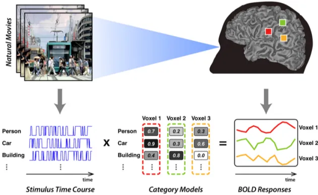
Figure 1. Voxelwise category models. A voxelwise modeling framework was used to measure category selectivity in single voxels from individual subjects. The WordNet lexicon was used to label salient object and action categories in each 1 s segment of the movies (Miller, 1995). This labeling procedure produced for each category a separate binary variable that indicates its presence/absence throughout the stimulus. The binary variables for 1705 distinct categories were taken as the stimulus features. Regularized linear regression was used to find a weighted sum of stimulus features that best describe the measured BOLD responses. The resulting model weights characterize the selectivity of single voxels to 1705 distinct object and action categories.
Motion-energy model. Many voxels throughout the visual system are
selective for elementary visual features, such as spatial location or spatio-temporal frequency. To measure selectivity for elementary features in single voxels, a motion-energy model was fit that was previously shown to accurately predict BOLD responses to natural movies in retinotopi-cally organized early visual areas (Nishimoto et al., 2011). This motion-energy model contained 2139 spatiotemporal Gabor filters. Each filter was a three-dimensional spatiotemporal sinusoid multiplied by a spa-tiotemporal Gaussian envelope. Filters were computed at six spatial frequencies (0, 1.5, 3, 6, 12, and 24 cycles/image), three temporal fre-quencies (0, 2, and 4 Hz), and eight directions (0, 45, 90, 135, 180, 225, 270, and 315°). Filters were positioned on a square grid that spanned 24⫻ 24°. Filters at each spatial frequency were placed on the grid such that adjacent filters were separated by a distance of 4 SDs of the spatial Gaussian envelope.
Model fitting. All voxelwise models were fit using regularized linear
regression with an l2-penalty on model weights to prevent overfitting.
The temporal sampling rates of the stimulus and BOLD responses were matched by down-sampling the stimulus time course twofold. Hemody-namic response functions were modeled separately for each model fea-ture using separate linear finite-impulse-response (FIR) filters. FIR filter delays were restricted to 4 – 8 s (equivalently 2– 4 samples), and FIR co-efficients were fit simultaneously with model weights to obtain high-quality fits.
A 10-fold cross-validation procedure was used to optimize model weights to predict BOLD responses in the training data (Fig. 1). In each fold, 10% of the training data were randomly held out, and the models were fit to the remaining data. Model performance was assessed on the held-out data by calculating prediction scores, i.e., the correlation coef-ficient (Pearson’s r) between the actual and predicted BOLD responses. The optimal regularization parameter for each voxel was determined by maximizing its prediction score. Finally, the optimal parameters were used to refit the models to all training data in a single step.
Model performance was assessed on independent test data using a jackknifing procedure. BOLD response predictions on the test data were randomly resampled 10,000 times without replacement (at a rate of 80%). Model performance was measured as the average prediction score across jackknife iterations. Model fitting was performed using custom software written in Matlab (MathWorks). When necessary, significance levels were corrected for multiple comparisons using false-discovery-rate control (Benjamini and Yekutieli, 2001).
Variance partitioning analysis. Objects and actions in natural movies
can be correlated with lower-level visual features. It is therefore possible that the category models estimated here might be biased by selectivity for low-level features in scene-selective ROIs. To check for this potential confound, we performed a variance partitioning analysis. This analysis corrects the response variance explained by the category model to ac-count for variance that can be attributed to low-level features captured by the gist or motion-energy models. To do this, we separately measured the variance explained when all three models (category, gist, and motion energy) are fit simultaneously, the variance explained when two models are fit simultaneously, and the variance explained by regressors of indi-vidual models. The proportion of variance for each model was calculated with respect to the variance explained by the simultaneous fit of all three models. Leveraging simple set-theoretic relations among the measure-ments, we extracted the proportion of unique variance explained by each model, and the proportion of shared variance explained commonly by multiple models.
Cluster analysis. The core issue that we address in this report concerns
whether category selectivity is heterogeneous across voxels located within scene-selective ROIs. To investigate this issue, we performed separate cluster analyses on voxelwise tuning profiles measured within the PPA, RSC, and OPA. The analyses were first run at the group level by pooling tuning profiles in each ROI across subjects. This group analysis yields common cluster labeling and facilitates comparisons among subjects. To ensure that the group clusters were consistent at a single subject level, cluster analyses were also repeated in individual subjects. The cluster solutions were compared by calculating the correlation coefficient be-tween the obtained cluster centers.
We examined the group structure among ROI voxels using a sensitive spectral-clustering algorithm (Ng et al., 2001). The dissimilarity between pairs of tuning profiles was characterized by a normalized Euclidean-distance measure. To determine the number of clusters in the data, we used an unsupervised stability-based validation method (Ben-Hur et al., 2002;Handl et al., 2005). This validation method repeats the clustering analyses for a given number of clusters on random subsamples of the data. The stability for a given number of clusters is measured as the similarity between the cluster solutions on different subsamples. By re-peating this procedure many times, the empirical probability distribu-tion of clustering stability is obtained. If the number of clusters is appropriate for the data, then the cluster solutions should be stable. In contrast, if a suboptimal number is chosen, then the cluster solutions should be unstable.
Here we estimated the probability distribution of clustering stability by a random subsampling procedure repeated 5000 times. To enhance sensitivity, this procedure was performed after pooling voxels within each area across subjects. During each repeat, 80% of voxels were ran-domly selected without replacement twice, and the cluster solutions of this pair of subsamples were compared. The similarity of the solutions was quantified using the Jaccard Index (Jaccard, 1908). The cumulative distribution of clustering stability was estimated using normalized histo-grams (for a bin width of 0.005) across 5000 repeats. In this analysis, distributions of stable cluster solutions will be concentrated around unity similarity values, whereas distributions of unstable solutions will be more variable. For this reason, we determined the optimal number of clusters by comparing the value of the cumulative distribution functions at a high stability threshold for different numbers of clusters (Ben-Hur et al., 2002;
C¸ukur et al., 2013b). A stability threshold of 0.9 was used here based on previously suggested values (Ben-Hur et al., 2002), but similar results were obtained for threshold values in the 0.80 – 0.95 range.
Functional importance of heterogeneous selectivity. Here we assessed
heterogeneous selectivity in scene-selective ROIs in two steps: we first fit encoding models to measure category selectivity in individual voxels; we then clustered the model weights to identify subdomains within each ROI. We performed two complementary analyses to evaluate both the functional importance of intervoxel differences in selectivity and inter-cluster differences in selectivity. First we asked whether individual voxels in each ROI show significant heterogeneity that would justify a cluster analysis. We reasoned that if model weights are significantly different across voxels, then a model fit to an individual voxel (self-prediction) should explain more of that voxel’s responses than is explained by models fit to other voxels within the ROI (cross-prediction). We thus compared self-prediction and cross-prediction in terms of the proportion of vari-ance explained in held-out test data.
Next we asked whether the voxel clusters within each ROI show func-tionally important differences in selectivity. If selectivity is significantly different across clusters, then a target voxel’s responses should be better explained by models fit to other voxels in the same cluster (within-cluster prediction) than it is by models fit to voxels in a different cluster (cluster prediction). Therefore we compared within-(cluster and cross-cluster prediction in terms of proportion of explained variance. This analysis was repeated by obtaining separate predicted responses using category, gist, and motion-energy models. In both analyses of heteroge-neity, the proportion of variance for each model was calculated with respect to the variance explained by the simultaneous fit of all three models. Significant differences were assessed with bootstrap tests.
Visualization of cluster centers. To interpret differences between the
cluster centers, we visualized the mean tuning profile of each cluster within its optimal model space. For the category model, a graphical tree was constructed to visualize category responses to distinct objects and actions. The vertices of the graph corresponded to 1705 distinct catego-ries. The connecting edges of the graph represented the hierarchical re-lationships between these categories as given by WordNet. The size and color of vertices represented the magnitude and sign of the category responses, respectively. For the motion-energy model, line plots were used to visualize the responses to distinct spatiotemporal frequencies.
Visualization on cortical surfaces. To understand the spatial
category selectivity onto flattened cortical surfaces. The surfaces were reconstructed in each individual subject from T1-weighted brain scans.
These anatomical data were processed in Caret for gray–white matter segmentation (Van Essen et al., 2001). Surfaces were constructed from the segmentations separately for each hemisphere. The cortical surfaces were then flattened after applying five relaxation cuts placed so as to minimize spatial distortion. To project voxelwise category models onto the generated flat maps, functional data were aligned to the anatomical data using in-house Matlab scripts (MathWorks). These scripts used affine transformations to manually coregister three-dimensional func-tional and anatomical datasets (Hansen et al., 2007).
Spatial segregation of voxel clusters. The cluster analysis procedure
de-scribed above was applied to voxelwise tuning profiles without including any information about the spatial location of the voxels. Thus, that anal-ysis alone does not provide any information about whether clusters iden-tified within scene-selective ROIs are spatially segregated in the cortex. If clusters are segregated spatially, then the three-dimensional anatomical distances among voxels within each cluster should be smaller than the distances among voxels between different clusters. In contrast, if clusters are intermingled, within-cluster and between-cluster distances should be similar. Therefore, to determine whether functionally distinct clusters are also clustered anatomically, we first measured the three-dimensional anatomical distance between every pair of voxels within each individual brain, and we then aggregated these distances within and between clus-ters separately. We used bootstrap tests to compare these distances to null distributions of within-cluster and between-cluster distances obtained by randomly shuffling the anatomical locations voxels in each individual ROI and in each individual brain.
Results
Representation of nonscene categories in the PPA, RSC,
and OPA
There is substantial evidence that the three scene-selective areas
examined here—the PPA, RSC, and OPA—represent
informa-tion about natural visual scenes (
Grill-Spector and Malach, 2004
;
Spiridon et al., 2006
;
Nasr et al., 2011
). However, these areas also
appear to represent information about nonscene categories
(
Huth et al., 2012
;
Stansbury et al., 2013
), though this is poorly
understood. Because natural scenes contain many distinct objects
and actions, elucidating the representations of objects and
ac-tions in scenes is a challenging problem. To investigate this issue,
we assessed selectivity for hundreds of object and action
catego-ries in the PPA, in the RSC, and in the OPA. We recorded BOLD
responses from six subjects who viewed 2 h of natural movies,
and we fit category models to each individual voxel in every
sub-ject. This enabled us to estimate voxelwise selectivity for 1705
separate object and action categories (
Fig. 1
). We find that the
category model yields significant prediction scores in all ROIs:
0.38
⫾ 0.08 in the PPA (correlation; mean ⫾ SD across subjects),
0.38
⫾ 0.09 in the RSC, and 0.40 ⫾ 0.06 in the OPA. All these
values are statistically significant ( p
⬍ 10
⫺4, bootstrap test). As a
control, we fit separate gist models that reflect voxelwise
selectiv-ity for the spatial texture and layout of visual scenes. The gist
model also yields significant prediction scores: 0.12
⫾ 0.03 in the
PPA, 0.11
⫾ 0.08 in the RSC, and 0.11 ⫾ 0.03 in the OPA (p ⬍
10
⫺4). However, the category model performs significantly
bet-ter than the gist model in all three ROIs ( p
⬍ 10
⫺4). These results
indicate that voxel responses in scene-selective areas carry
signif-icant information about object and action categories in natural
scenes.
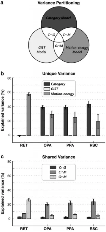
Figure 2. Selectivity for object and action categories. a, Three separate models were esti-mated for each voxel: a category model that describes selectivity for object and action catego-ries; a gist model that describes selectivity for spatial structures of scenes; and a motion-energy model that describes selectivity for low-level visual features. Models were validated by predict-ing BOLD responses in a separate dataset reserved for this purpose. A variance partitionpredict-ing analysis was used to estimate the proportion of response variance predicted uniquely by each model and jointly by multiple models (see diagram). b, The proportion of variance explained uniquely by category, gist, and motion-energy models in each ROI (mean⫾ SEM across sub-jects). In early retinotopic visual areas (RET), the category model does not explain variance beyond what can be attributed to selectivity for spatial structure or low-level visual features. In contrast, the category model explains a significant portion of variance in scene-selective ROIs ( p⬍ 10⫺4, bootstrap test). This result suggests that selectivity for nonscene categories in the PPA, RSC, and OPA cannot be fully explained by selectivity for spatial structure captured by the gist model or selectivity for low-level visual features captured by the motion-energy model. c, The proportion of variance explained commonly by category/gist (C艚G), category/motion-energy (C艚M), and gist/motion-energy (G艚M) models in each ROI (mean ⫾ SEM
4
across subjects). A relatively small portion of variance is explained jointly by category and motion-energy models (p⬍ 10⫺4). Therefore, to reduce spurious correlations, a nuisance motion-energy regressor was included in the category models during subsequent analyses.
While early visual areas are commonly
thought to represent low-level stimulus
features (
Grill-Spector and Malach, 2004
;
Kay et al., 2008
), recent studies suggest
that downstream scene-selective areas
might represent both low-level features
(
Rajimehr et al., 2011
) and global spatial
structure (
Walther et al., 2009
,
2011
;
Kravitz et al., 2011b
). Because objects and
actions in natural movies are partly
corre-lated with low-level features, the category
models estimated in scene-selective ROIs
might be biased. Thus we sought to
deter-mine whether the category model still
ex-plains a significant portion of the response
variance in the PPA, RSC, and OPA, after
accounting for variance that can be
attrib-uted to low-level features or scene
struc-ture. We used a variance partitioning
analysis to address this issue (
Fig. 2
a; see
Materials and Methods). The variance
partitioning analysis included three
sepa-rate models: the category and gist models
discussed above and a separate
motion-energy model that characterizes voxel
se-lectivity for low-level structural features,
including spatial position, spatiotemporal
frequency, and orientation. We calculated
the proportion of shared variance
ex-plained by multiple models and the
pro-portion of variance explained uniquely by
each model.
We performed the variance
partition-ing analysis for each of our subjects
indi-vidually, focusing on retinotopically
organized early visual areas (V1–V3) and
the PPA, RSC, and OPA (
Fig. 2
b). If the
category model explains a portion of the
response variance that cannot be
attrib-uted to the motion-energy or gist models,
then addition of the category model
re-gressors
should
improve
the
total
explained variance. We find that the
per-centage of explained variance that can be
attributed uniquely to the category model
is 39.4
⫾ 7.3% (mean ⫾ SD across
sub-jects) in the PPA, 43.8
⫾ 11.0% in the
RSC, and 39.2
⫾ 6.7% in the OPA (p ⬍
10
⫺4, bootstrap test), but it is
insignifi-cant in retinotopic areas ( p
⬎ 0.3). This
result suggests that scene-selective areas
represent significant information about
object and action categories in natural
scenes. Importantly, the variance
parti-tioning procedure ensures that this information cannot be
attrib-uted to selectivity for low-level features as reflected in the gist or
motion-energy models. At the same time a relatively small
por-tion of variance is explained commonly by category and mopor-tion-
motion-energy models ( p
⬍ 10
⫺4;
Fig. 2
c). Therefore, to reduce spurious
correlations in subsequent analyses presented in this paper, a
nuisance motion-energy regressor was included in the category
models (see Materials and Methods).
Functional heterogeneity in the PPA, RSC, and OPA
Several recent studies report that subregions within the PPA vary
in their visual responsiveness and spatial-frequency tuning (
Ar-caro et al., 2009
;
Rajimehr et al., 2011
;
Baldassano et al., 2013
).
These findings suggest that the PPA, and perhaps other
scene-selective ROIs, might contain multiple subdivisions with
differ-ent category selectivity. To test this heterogeneity hypothesis, we
first sought to determine whether individual voxels in the PPA,
RSC, and OPA differ in their tuning for object and action
catego-Figure 3. The optimal number of clusters for each scene-selective ROI. An unsupervised stability-based validation technique was used to determine the optimal number of clusters in three scene-selective ROIs. a, Cluster analysis for the PPA. Left, The cumulative distribution function of clustering stability, FJ( j), shown as a function of number of clusters (k) ranging from 2 to 7.Right, Change in value of FJacross consecutive k at a stability threshold of J⫽ 0.9 (Ben-Hur et al., 2002). The optimal k was
identified by detecting a sudden transition from narrow to widespread distributions. This transition was identified by a large increase in the value of FJwhen gradually increasing the number of clusters. The optimum number of clusters in the PPA is two
(data are aggregated across subjects and hemispheres). b, Cluster analysis for the RSC. Format same as in a. The optimum number of clusters in the RSC is two. c, Cluster analysis for the OPA. Format same as in a. The optimum number of clusters in the OPA is two.
ries. We reasoned that if model weights are significantly different
across voxels within an ROI, then the category model fit to an
individual voxel (i.e., self-prediction) should explain more of that
voxel’s response than can be explained using category models fit
to other voxels (i.e., cross-prediction). Comparison of the
self-prediction and cross-self-prediction performance of category models
in all voxels within each ROI shows that self-prediction
im-proves explained variance by 24.1
⫾ 9.5% in the PPA (mean ⫾
SD across subjects), by 28.5
⫾ 11.0% in the RSC, and by
25.0
⫾ 15.4% in the OPA (p ⬍ 10
⫺4, bootstrap test). These
results confirm that voxels within the PPA, RSC, and OPA are
functionally heterogeneous.
We next tested whether the heterogeneously tuned voxels in
scene-selective ROIs form distinct functional clusters. To do this,
we first applied spectral clustering to the voxelwise category
model weights obtained within each area. We performed a
stability-based validation procedure to determine the optimal
number of clusters in the PPA, RSC, and OPA separately, and we
measured cluster stability by repeating the cluster analysis 5000
times on subsets of voxels selected randomly in each random
draw (see Materials and Methods). We find that in all three ROIs,
the optimal number of clusters based on the category model is
two (
Fig. 3
; for voxel numbers across clusters, see
Table 1
). To
determine whether these clusters are consistent across subjects,
we measured the intersubject correlation of cluster centers, where
the cluster center was taken as the average model weight within a
cluster. We find that individual-subject clusters are highly
con-sistent across subjects (r
⫽ 0.84 ⫾ 0.04 in the PPA, 0.81 ⫾ 0.03 in
the RSC, and 0.72
⫾ 0.04 in the OPA; mean ⫾ SD across subjects,
p
⬍ 10
⫺4, bootstrap test), and that they are consistent with the
group clusters (0.92
⫾ 0.03 in the PPA, 0.91 ⫾ 0.02 in the RSC,
and 0.87
⫾ 0.04 in the OPA, p ⬍ 10
⫺4). For comparison, we also
performed the same cluster analysis procedure separately using the
gist model and the motion-energy model. In all three ROIs, the
op-timal number of clusters based on the gist and motion-energy
mod-els is one. Together, these results confirm that voxmod-els within the PPA,
RSC, and OPA are functionally clustered according to their category
selectivity, but they are not clustered for lower-level features.
We next examined whether the differential category selectivity
between these two voxel clusters are functionally important. We
reasoned that if the intercluster differences are important, a target
voxel’s responses should be better explained by models fit to
other voxels in the same cluster (within-cluster prediction) than
by models fit to voxels in a different cluster (cross-cluster
predic-tion). Therefore, we simply compared the within-cluster and
cross-cluster prediction performance in the PPA, RSC, and OPA.
Separate response predictions were obtained using category, gist,
and motion-energy models (
Fig. 4
). We find that within-cluster
performances based on category models are significantly higher
than cross-cluster performances in all three ROIs ( p
⬍ 0.001,
bootstrap test). For category models, percentage improvement in
explained variance is 6.3
⫾ 3.6% (mean ⫾ SEM across subjects)
in the PPA, 6.0
⫾ 3.2% in the RSC, and 9.6 ⫾ 3.6% in the OPA.
These results strongly support the hypothesis that there are two
functional subdomains with distinct category tuning in the PPA,
RSC, and OPA.
To examine the differences in category tuning between these
subdomains, we first visualized the cluster center weights for
1705 categories in each scene-selective ROI (
Fig. 5
for group
cen-ters; see
Figs. 12
–
14
for individual-subject centers).
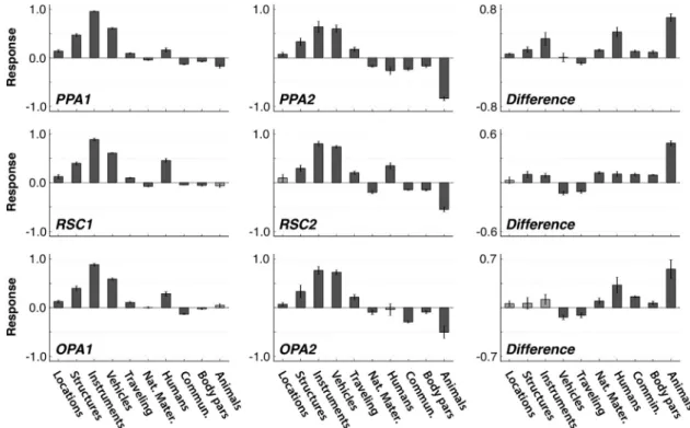
Figure 6
sum-marizes the responses of each cluster to several important object
and action categories, along with response differences between
the two clusters. BOLD responses of both the first and second
cluster in each ROI (here denoted as PPA1, RSC1, and OPA1 for
cluster 1, and PPA2, RSC2, and OPA2 for cluster 2) increase when
structures, man-made instruments, vehicles, and movement are
present ( p
⬍ 0.001, bootstrap test). Responses of these same
clusters are reduced by scenes presenting social communication,
such as people talking or gesturing ( p
⬍ 0.001). Furthermore,
both clusters yield greater responses for man-made instruments
and vehicles than for buildings and geological formations ( p
⬍
0.001). However, in every ROI the two functional clusters differ
in their relative responses to these categories and to other
ecolog-ically relevant categories. Specifecolog-ically, the first cluster (PPA1,
RSC1, and OPA1) produces relatively greater responses than the
second cluster when natural materials, body parts, humans,
ani-mals, and social communication are present in the movies ( p
⬍
0.05). In contrast, the first cluster produces relatively reduced
responses when the movies show movement, such as a moving
car or train, or a walking person ( p
⬍ 0.001). Furthermore,
re-sponses in the RSC1 and OPA1 are reduced when vehicles are
present ( p
⬍ 0.001). These results suggest that the first
sub-domain in scene-selective areas has stronger tuning for animate
objects and man-made instruments, while the second subdomain
is relatively more tuned for vehicles and action categories that
appear in dynamic visual scenes.
Table 1. Distribution of voxels across clusters identified in scene-selective ROIs
PPA1 PPA2 RSC1 RSC2 OPA1 OPA2
Total 277 243 185 228 223 184 S1 11 88 16 54 4 49 S2 36 11 13 19 7 6 S3 39 34 52 66 62 46 S4 59 28 13 22 68 30 S5 91 73 19 49 38 42 S6 41 9 72 18 44 11
The first row shows the total number of voxels within each cluster, pooled across subjects. Subsequent rows show the number of voxels within each cluster in individual subjects (S1–S6).
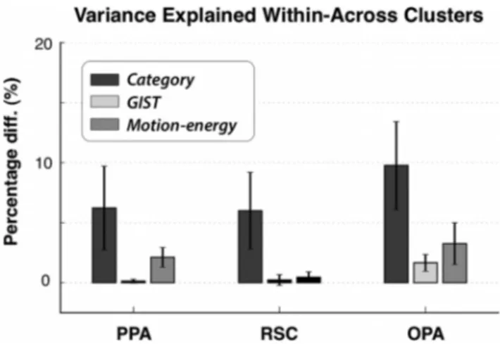
Figure 4. Functional segregation of subdomains. If subdomains identified within an ROI are functionally distinct, then the variance of a voxel’s response explained by other voxels in the same subdomain (within-subdomain prediction) should be greater than the variance explained by voxels in different subdomains (cross-subdomain prediction). We therefore compared within-prediction and cross-prediction performances based on responses predicted by the cat-egory, gist, and motion-energy models. Bar plots show the percentage difference in explained variance in the PPA, RSC, and OPA (mean⫾SEMacrosssubjects).Greaterpercentagesindicate better within-prediction than cross-prediction performance. Insignificant differences are shown in blank outlines ( p⬎ 0.05). In all ROIs, the within-prediction performance of the category model is greater than the cross-prediction performance ( p⬍ 0.001, bootstrap test). This result suggests that there are functional subdomains with distinct category tuning in the PPA, RSC, and OPA.
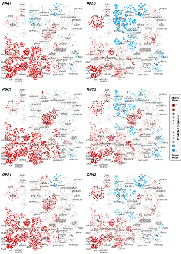
Figure 5. Category tuning of the voxel clusters. Category tuning of the two functional subdomains identified in each scene-selective ROI. For each cluster, category tuning was taken as the mean tuning profile of all voxels within the ROI (data are aggregated across subjects and hemispheres). Tuning for 1705 categories are shown here using graphs that consist of separate trees for object (main tree, circular vertices) and action (smaller trees, square vertices) categories. To orient the reader, a subset of the categories has been labeled. The size of each vertex indicates the magnitude while its color indicates the sign (red,⫹; blue, ⫺) of the category response relative to the mean overall response. Left, Responses of PPA1, RSC1, and OPA1 are (Figure legend continues.)
Several recent studies have reported variability in visual
selec-tivity across the anterior–posterior axis of the PPA that also
ex-tends into neighboring patches of the cortex (
Arcaro et al., 2009
;
Rajimehr et al., 2011
;
Baldassano et al., 2013
). It is therefore
possible that category tuning follows a similar organization
within and nearby the three scene-selective areas examined here.
Alternatively, voxel clusters may show a patchy, noncontiguous
spatial distribution (
Grill-Spector et al., 2006
). To examine this
issue, we measured the category tuning profiles of all voxels
within a 40 mm radius of the geometric center of each
scene-selective ROI in each hemisphere. Separate principal component
(PC) analyses on category tuning profiles of voxels located within
each cluster reveal that the two clusters are clearly distinguished
by the first PC in each of the three ROIs (see below, PC analyses of
category models). To visualize these patterns, we mapped the first
PC projections of 1705-dimensional tuning profiles onto the
cor-tical surface. In
Figure 7
, voxels that belong to PPA1, RSC1, and
OPA1 have positive projections onto the first PC, while voxels in
PPA2, RSC2, and OPA2 have negative projections. Inspection of
these projections on cortical flatmaps suggests that voxels in the
first cluster tend to be located approximately in posterior-lateral
regions, and voxels in the second cluster tend to be located more
anteriomedially. Supporting this observation, a statistical
analy-sis indicates that there is significant spatial segregation between
the two clusters ( p
⬍ 0.01, bootstrap test; see Materials and
Methods). On the other hand, this segregation is not complete
and some degree of intermixing between the clusters appears to
occur within each ROI. Together, these results imply that
cate-gory representation across the PPA, RSC, and OPA are likely
organized by both monotonic gradients and distributed peaks of
selectivity.
PC analyses of category models
Evidence from recent studies suggests that the human brain
em-beds visual categories into a relatively low-dimensional semantic
space mapped systematically across the cortical surface (
Haxby et
al., 2011
;
Huth et al., 2012
). To obtain a data-driven description
of the semantic information represented in scene-selective areas,
we performed PC analyses across voxelwise category models. We
assessed the consistency of representations across subjects by
evaluating the cross-subject correlations between the PCs
esti-mated for individual subjects (
Huth et al., 2012
). To avoid
stimulus-sampling bias, we measured correlations between PCs
that were estimated separately from responses to the first and
second halves of the movies. We find that the first three
individual-subject PCs are highly correlated across subjects (r
⫽
0.61
⫾ 0.02 in the PPA, 0.54 ⫾ 0.01 in the RSC, and 0.57 ⫾ 0.01
in the OPA; mean
⫾ SD across subjects, p ⬍ 10
⫺4, bootstrap
test). These individual-subject PCs are also highly correlated with
the group PCs in all three areas (0.71
⫾ 0.03 in the PPA, 0.62 ⫾
0.01 in the RSC, and 0.64
⫾ 0.02 in the OPA, p ⬍ 10
⫺4).
Our cluster analyses indicate that voxels in each of the three
ROIs form two clusters that differ in their category tuning. To
examine the semantic dimensions that capture these tuning
dif-ferences, we projected the voxelwise tuning profiles onto the first
4
(Figure legend continued.) strongly increased by the presence of man-made instruments, devices, vehicles, structures, roads, and locations (e.g., city, grassland), and they are weakly increased by the presence of humans. Right, Responses of PPA2, RSC2, and OPA2 are strongly increased by the presence of vehicles, roads, and traveling, and they are strongly reduced by animals, plants, natural materials, body parts, and communication.
Figure 6. Predicted differences in category responses across clusters. The voxelwise category models fit to all voxels within each subdomain were used to estimate predicted responses to geographic locations, structures (e.g., building), instruments, vehicles, movement, natural materials, humans, social communication, body parts, and animals. The response level for each of these superordinate categories was taken as the average response across all of its subordinate categories included in the category model. Bar plots show the response level (mean⫾ SEM across subjects) for the two subdomains in each ROI as well as their difference (right column). Significant responses are shown in dark gray (p⬍ 0.05, bootstrap test) and insignificant responses are shown in light gray. Relative to the second subdomain, the first subdomain is observed to respond less to traveling, and relatively more to most of the remaining categories including those related to humans, communication, and structures.
Figure 7. Cortical flatmaps of category selectivity within and outside scene-selective ROIs. To examine the spatial distribution of category selectivity, category tuning profiles were measured for voxels within and around the PPA, RSC, and OPA separately. The tuning profiles in the vicinity of each ROI were then projected onto the first group PC (calculated only from voxels within the given ROI). Here the projections obtained for the PPA, RSC, and OPA are shown on separate cortical flatmaps for two representative subjects S2 and S6. Brain areas identified using functional localizers are labeled and their extent is delineated with white lines. Voxels with positive projections onto the PC (i.e., category tuning more similar to PPA1, RSC1, and OPA1) appear in red, and voxels with negative projections (i.e., category tuning more similar to PPA2, RSC2 and OPA2 appear in blue. The two voxel clusters in each ROI show spatial segregation on the cortical surface.
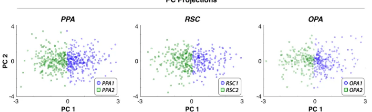
Figure 8. Projections of voxelwise tuning profiles onto PCs. To independently assess the functional heterogeneity in scene-selective ROIs, voxelwise tuning profiles were projected onto the first two group PCs obtained from voxels within each ROI (data aggregated across subjects and hemispheres). Each voxel in the first cluster (PPA1, RSC1, and OPA1) is denoted with a blue circle, and each voxel in the second cluster (PPA2, RSC2, and OPA2) is denoted with a green square. Voxels in separate clusters are spatially segregated in the PC space. Projections onto the first PC clearly separate voxels in the first and second clusters, implying that category representation in scene-selective ROIs is organized according to at least one semantic dimension.
two group PCs of category models in each area. Across subjects,
the first and second PCs explain 48.4
⫾ 10.8% and 15.1 ⫾ 2.6% of
category responses in the PPA, 48.1
⫾ 8.9% and 15.7 ⫾ 4.3% in
the RSC, and 58.9
⫾ 9.1% and 14.2 ⫾ 5.7% in the OPA. This
result indicates that voxels in separate clusters project to
segre-gated regions in the semantic space defined by the selected PCs
(
Fig. 8
). Inspection of
Figure 8
reveals that the first PC clearly
captures the differences in category tuning between the two
clus-ters in the PPA, RSC, and OPA. As shown in
Figure 9
, this first PC
appears to contrast categories related to civilization (e.g.,
instru-ments, vehicles, roads, indoor spaces, and humans) with
catego-ries related to social interaction (e.g., communication) and
outdoor activities (e.g., outdoor events, movement, and natural
materials). While a more precise interpretation of PCs across a
1705-dimensional feature space is naturally difficult, our results
suggest that category representation is organized consistently
across subjects according to at least one semantic dimension.
Hemispheric symmetry of category representations
Several previous studies suggest that brain function in
category-selective areas in the high-level visual cortex are lateralized across
hemispheres (
Rossion et al., 2000
;
Stevens et al., 2012
). We
there-fore asked whether the voxel clusters identified in the PPA, RSC,
or OPA are lateralized. To address this issue, we first counted the
number of voxels included in the definition of scene-selective
areas in the left and the right hemispheres separately. We find no
consistent hemispheric lateralization in ROI definitions across
subjects for the PPA ( p
⬎ 0.15, bootstrap test). However, 73.7 ⫾
11.4% of all RSC voxels and 66.4
⫾ 26.9% of all OPA voxels
(mean
⫾ SD across subjects) are located in the right hemisphere
( p
⬍ 0.05). We next examined the distribution of voxels across
the two hemispheres for individual clusters (subjects S1 and S2
had no OPA voxels in the left hemisphere and so were omitted
from this analysis). For each cluster, we computed the ratio of the
voxels in a given hemisphere to the total number of voxels across
both hemispheres. We find that there is no significant
lateraliza-tion for either of the two clusters in the PPA, RSC, or OPA ( p
⬎
0.30, bootstrap test). This result indicates that subdomains in
scene-selective areas are relatively balanced across cerebral
hemispheres.
Control analyses for potential confounds caused by bias in
the movie stimulus
We report here that the mean category tuning profiles of the voxel
clusters are highly consistent across individual subjects in the
PPA, RSC, and OPA. However, we were concerned that these
results might be an artifact of statistical bias in the natural movies
used as stimuli in the main experiment. After all, voxelwise
tun-ing profiles were measured ustun-ing responses elicited by the same
stimulus in all subjects. Any natural stimulus of finite duration
will inevitably reflect some degree of stimulus sampling bias and,
if this bias is significant, then it might increase the apparent
sim-ilarity of model weights calculated across subjects. To rule out
this potential bias, we fit separate models to responses recorded
during the first and second halves of the movie. The clips used in
the first and second halves of the movie were completely
unre-lated, so if the results are consistent across the two halves then it
would suggest that statistical bias in the movies is not an
impor-tant concern. We ran cluster analyses individually on each set of
models, and we compared the resulting cluster centers. We find
that the split-half cluster centers are strongly correlated across
subjects (r
⫽ 0.79 ⫾ 0.04 in the PPA, 0.75 ⫾ 0.01 in the RSC, and
0.60
⫾ 0.07 in the OPA, mean ⫾ SD, p ⬍ 10
⫺4, bootstrap test).
This result indicates that the consistency of clusters across
sub-jects is unlikely to be due to stimulus sampling bias.
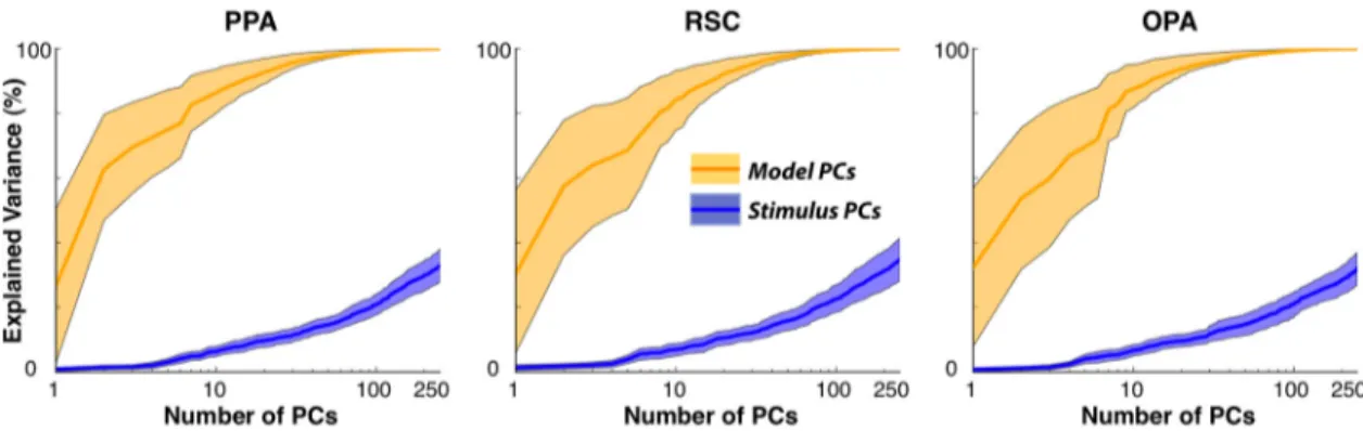
Another potential confound stems from the correlations
among different categories in the finite movie stimulus used in
this study. Multiple distinct categories of objects and actions may
co-occur in natural movies. If these category correlations are
large, then the corresponding category regressors used in our
voxelwise models will be highly correlated, which might bias the
fit model weights. To assess the effect of category correlations on
model fits, we measured the amount of variance in the voxelwise
category model weights that can be attributed to the stimulus
time course. To account for temporally lagged correlations, we
concatenated multiple delayed time courses for all 1705
catego-Figure 9. Group PCs of tuning profiles in scene-selective ROIs. PC weights for the PPA, RSC, and OPA. Tuning diagrams are formatted as inFigure 5. Inspection of the tuning diagrams of the first PC reveals the semantic dimension that distinguishes the two subdomains in each scene-selective ROI. The first PC approximately contrasts categories related to human civilization and man-made artifacts (e.g., instruments, vehicles, roads, indoor spaces, and humans) with categories related to social interaction (e.g., communication) and outdoor activities (e.g., outdoor events, movement, and natural materials). Thus the first subdomain tuned for objects commonly appearing in static scenes has positive projections onto this PC, while the second subdomain tuned for object and actions in dynamic scenes has negative projections.ries with lags ranging between
⫺5 and 5 s.
We then calculated PCs of the resulting
stimulus matrix, and separately calculated
the PCs of the category model weights. If
stimulus correlations strongly bias the
model fits, then the stimulus PCs should
explain a comparable portion of the
vari-ance in the model weights to that
ex-plained by the model PCs. We find that
model PCs explain a significantly larger
portion of the variance compared with the
stimulus PCs (
Fig. 10
; p
⬍ 10
⫺4,
boot-strap test). In each ROI, we compared the
combined explanatory power of all model
PCs (total of 10 PCs) that individually
ex-plain
⬎1% of the variance in model
weights with all stimulus PCs (total of 20
PCs) that each explain
⬎1% of variance in
the stimulus matrix. We find that the
vari-ance in model weights explained by model
PCs is 87.0
⫾ 3.3% in the PPA (mean ⫾
SD across subjects), 83.9
⫾ 3.2% in the
RSC, and 87.6
⫾ 3.0% in the OPA. In
con-trast, the variance in model weights
ex-plained by stimulus PCs was substantially
smaller ( p
⬍ 10
⫺4, bootstrap test), merely
8.7
⫾ 0.9% in the PPA, 9.9 ⫾ 0.8% in the
RSC, and 9.1
⫾ 1.2% in the OPA. This
result indicates that the estimated
voxel-wise category model weights are not
bi-ased by category correlations in the movie
stimulus.
One final potential confound concerns
the correlation between low-level
struc-tural and high-level categorical features in
natural scenes. If scene-selective areas
represent low-level visual features (such
as spatiotemporal frequency or
orienta-tion) that differ systematically across
cat-egories, then the category model weights
might be biased. Of particular concern for
this study is the possibility that the
heter-ogeneity of category tuning across an area
could reflect heterogeneity of tuning for
Figure 10. Temporal stimulus correlations between categories in natural movies. Regressors for multiple distinct categories of objects and actions may be correlated in the natural movie stimulus. To assess the effect of category correlations on our model fits, we compared the PCs of model weights with the PCs of the stimulus time course in terms of the amount of variance they can explain in voxelwise category models. Plots show the mean and 68th-percentile bands of the explained variance across the population of voxels in each ROI. Regardless of the number of PCs used, model PCs account for a significantly larger proportion of variance in the model weights compared with stimulus PCs (p⬍ 10⫺4, bootstrap test). This result indicates that the estimated voxelwise category model weights are not biased by category correlations in the movie stimulus.
Figure 11. Motion-energy tuning of the voxel clusters. Differences in category tuning between the voxel clusters could poten-tially be confounded by differences in tuning for low-level structural features. To examine this issue, the mean motion-energy tuning of the clusters identified inFigure 5were calculated for the PPA, RSC, and OPA separately. Spatial-frequency and velocity tuning profiles of the first (PPA1, RSC1, OPA1) and second (PPA2, RSC2, OPA2) voxel clusters are denoted with blue and green lines, respectively. Error bars indicate SEM across voxels in each cluster. There are no significant differences in spatial frequency or velocity tuning of the two clusters in any of the three ROIs (p⬎0.05,bootstraptest).Thisresultsuggeststhatdifferencesincategorytuning between the two subdomains identified in the PPA, RSC, and OPA cannot be attributed to heterogeneity of motion-energy tuning.