Modified Korteweg–de Vries surfaces
Süleyman Teka兲
Department of Mathematics, Faculty of Science, Bilkent University, 06800 Ankara, Turkey
共Received 14 September 2006; accepted 13 November 2006; published online 23 January 2007兲
In this work, we consider 2-surfaces inR3arising from the modified Korteweg–de Vries共mKdV兲 equation. We give a method for constructing the position vector of the mKdV surface explicitly for a given solution of the mKdV equation. mKdV surfaces contain Willmore-like and Weingarten surfaces. We show that some mKdV surfaces can be obtained from a variational principle where the Lagrange function is a polynomial of the Gaussian and mean curvatures. © 2007 American Institute of
Physics. 关DOI:10.1063/1.2409523兴
I. INTRODUCTION
In this work we study the 2-surfaces in R3 arising from the deformations of the modified
Korteweg–de Vries共mKdV兲 equation and its Lax pair. Deformation technique was developed by several authors. Here we mainly follow Refs.1–12.
Let u共x,t兲 satisfy the mKdV equation
ut= u3x+
3 2u
2u
x. 共1兲
Substituting the traveling wave ansatz ut−␣ux= 0 in Eq.共1兲, where␣is an arbitrary real constant, we get
u2x=␣u − u3
2 . 共2兲
Here and in what follows, subscripts x, t, and denote the derivatives of the objects with respect to x, t, and, respectively. The subscript nx stands for n times x derivative, where n is a positive integer, e.g., u2xindicates the second derivative of u with respect to x. We use Einstein’s
summa-tion convensumma-tion on repeated indices over their range. Equasumma-tion共2兲can be obtained from a Lax pair
U and V, where U = i 2
冉
− u − u −冊
, 共3兲 V = − i 2冉
1 2u 2−共␣+␣ + 2兲 共␣+兲u − iu x 共␣+兲u + iux − 1 2u2+共␣+␣ + 2兲冊
, 共4兲and is the spectral parameter. The Lax equations are given as
a兲Electronic mail: [email protected]
48, 013505-1
⌽x= U⌽, ⌽t= V⌽, 共5兲 where the integrability of these equations are guaranteed by the mKdV equation or the zero curvature condition
Ut− Vx+关U,V兴 = 0. 共6兲
A connection of the mKdV equation to surfaces inR3 can be achieved by defining su共2兲 valued
2⫻2 matrices A and B satisfying
At− Bx+关A,V兴 + 关U,B兴 = 0. 共7兲
Let F be an su共2兲 valued position vector of the surface S corresponding to the mKdV equation such that
yj= Fj共x,t;兲, j = 1,2,3, F = i
兺
k=1 3Fkk, 共8兲
wherek’s are the Pauli sigma matrices
1=
冉
0 1 1 0冊
, 2=冉
0 − i i 0冊
, 3=冉
1 0 0 − 1冊
. 共9兲The connection formula共connecting integrable systems to 2-surfaces in R3兲 is given by
Fx=⌽−1A⌽, Ft=⌽−1B⌽. 共10兲 Then at each point on S, there exists a frame 兵Fx, Ft,⌽−1C⌽其 forming a basis of R3, where C =关A,B兴/储关A,B兴储and关A,B兴 denotes the usual commutator 关A,B兴=AB−BA. The inner product 具,典 of su共2兲 valued vectors X and Y are given by 具X,Y典=−1
2tr共XY兲. Hence储X储=
冑
兩具X,X典兩. The firstand second fundamental forms of S are
共dsI兲2⬅ gijdxidxj=具A,A典dx2+ 2具A,B典dxdt + 具B,B典dt2,
共11兲 共dsII兲2⬅ hijdxidxj=具Ax+关A,U兴,C典dx2+ 2具At+关A,V兴,C典dxdt + 具Bt+关B,V兴,C典dt2, where i , j = 1 , 2, x1= x, and x2= t. Here gij and hij are coefficients of the first and second funda-mental forms, respectively. The Gauss and the mean curvatures of S are, respectively, given by
K = det共g−1h兲 and H=1
2tr共g−1h兲, where g and h denote the matrices 共gij兲 and 共hij兲, and g−1stands for the inverse of the matrix g.
In order to calculate the fundamental forms in Eq.共11兲and the curvatures K and H, one needs the deformation matrices A and B. Given U and V, finding A and B from Eq.共7兲is a difficult task in general. However, there are some deformations which provide A and B directly. They are given as follows:
• Spectral parameter invariance of the equation:
A =U , B = V , F =⌽−1 ⌽ , 共12兲
whereis an arbitrary function of.
• Symmetries of the共integrable兲 differential equations:
A =␦U, B =␦V, F =⌽−1␦⌽, 共13兲
where␦ represents the classical Lie symmetries and共if integrable兲 the generalized symme-tries of the nonlinear partial differential equations共PDEs兲.
A = Mx+关M,U兴, B = Mt+关M,V兴, F = ⌽−1M⌽, 共14兲 where M is any traceless 2⫻2 matrix.
There are some surfaces which may be obtained from a variational principle. For this purpose, we consider a functionalF which is defined by
F ⬅
冕
SE共H,K兲dA + p
冕
VdV, 共15兲
whereE is some function of the curvatures H and K, p is a constant, and V is the volume enclosed by the surface S. For open surfaces, we let p = 0. The first variation of the functionalF gives the following Euler-Lagrange equation for the Lagrange functionE:13–16
共ⵜ2+ 4H2− 2K兲E
H+ 2共ⵜ · ⵜ¯ + 2KH兲
E
K− 4HE + 2p = 0, 共16兲
whereⵜ2andⵜ·ⵜ¯ are defined as
ⵜ2= 1
冑
˜g xi冉
冑
˜gg ij xj冊
, ⵜ · ⵜ¯ = 1冑
˜g xi冉
冑
˜Khg ij xj冊
, 共17兲and g˜ = det共gij兲, where gijand hijare the inverse components of the first and second fundamental forms, x1= x, x2= t. The following are examples of surfaces derived from a variational principle:
共i兲 Minimal surfaces:E=1, p=0;
共ii兲 constant mean curvature surfaces:E=1;
共iii兲 linear Weingarten surfaces:E=aH+b, where a and b are some constants; 共iv兲 Willmore surfaces:E=H2;17,18 and
共v兲 surfaces solving the shape equation of lipid membrane: E=共H−c兲2, where c is a
constant.13–16,19–21
The surfaces obtained from the solutions of the equation
ⵜ2H + aH3+ bHK = 0 共18兲
are called Willmore-like surfaces, whereⵜ2is the Laplace-Beltrami operator defined on the surface
and a , b are arbitrary constants. Unless a = 2 and b = −2, these surfaces do not arise from a varia-tional problem. The case a = −b = 2 corresponds to the Willmore surfaces. For compact 2-surfaces, the constant p may be different than zero, but for noncompact surfaces we assume it to be zero. For the latter, we require asymptotic conditions, where K goes to a constant and H goes to zero. This requires that the mKdV equation have solutions decaying rapidly to zero as兩x兩→ ±⬁. Soliton solutions of the mKdV equation satisfy this requirement. In this work, using solitonic solutions of the mKdV equation, we find the corresponding 2-surfaces and then solve the Euler-Lagrange equation关Eq. 共16兲兴 for polynomial Lagrange functions of H and K, i.e.,
E = aNHN+ ¯ + b10KH + b11KH2+ ¯ + e1K + . . . . 共19兲
For each N, we find the constants al, bnk, and em in terms of others and the parameters of the surface.
From a solution of the mKdV equation, we first find the fundamental forms in Eq.共11兲and the curvatures K and H of the corresponding 2-surface S. To find the position vector y共x,t兲 of S, we use Eq.共10兲. To solve this equation, we need the matrix⌽ satisfying the Lax equation 关Eq.共5兲兴 for a given function u共x,t兲. Hence, in general, our method for constructing the position vector y of integrable surfaces consists of the following steps:
共ii兲 Find a solution of the Lax equation关Eq.共5兲兴 for a given u共x,t兲.
共iii兲 Find the corresponding deformation matrices A, B, and find F from Eq.共10兲.
In this work more specifically, starting with one soliton solution of the mKdV equation and following the steps above, we solve the Lax equations and find the corresponding SU共2兲 valued function⌽共x,t兲. Then using the spectral deformations and combination of the gauge and spectral deformations, we find the parametric representations共position vectors兲 of the mKdV surfaces and plot some of them for some special values of constants. We show that there are some Weingarten and Willmore-like mKdV surfaces obtained from spectral deformations. Surfaces arising from a combination of the gauge and spectral deformations do not contain Willmore-like surfaces. We study also the mKdV surfaces corresponding to the symmetry deformations. We determine all geometric quantities in terms of the function u共x,t兲 and the symmetry 共x,t兲. For the simplest symmetry = ux, the surface turns out to be the surface of the sphere with radius 兩共␣兲/共2兲兩, where is the spectral parameter and␣ and are constants.
II. mKdV SURFACES FROM SPECTRAL DEFORMATIONS
In this section, we find surfaces arising from the spectral deformation of Lax pair for the mKdV equation. We start with the following proposition.
Proposition 1: Let u satisfy (which describes a traveling mKdV wave) Eq. (2). The corre-sponding su共2兲 valued Lax pair U and V of the mKdV equation are given by Eqs. (3) and (4), respectively. Then, su共2兲 valued matrices A and B are
A = i 2
冉
0 0 −冊
, 共20兲 B = − i 2冉
−共␣+ 2兲 u u ␣+ 2冊
, 共21兲where A =U, B =V, is a constant, and is the spectral parameter. The surface S, gener-ated by U, V, A and B, has the following first and second fundamental forms共j,k=1,2兲:
共dsI兲2= gjkdxjdxk= 2 4 共关dx + 共␣+ 2兲dt兴 2+ u2dt2兲, 共22兲 共dsII兲2= hjkdxjdxk= u 2 共dx + 共␣+兲dt兲 2+u 4 共u 2− 2␣兲dt2, 共23兲 with the corresponding Gaussian and mean curvatures
K = 2 2共u2− 2␣兲, H = 1 2u共3u 2+ 2共2−␣兲兲, 共24兲 where x1= x , x2= t.
By using U, V, A, and B and the method given in Sec. I, Proposition 1 provides the first and second fundamental forms, and the Gaussian and mean curvatures of the surface corresponding to spectral deformation. The following proposition gives a class of surfaces which are Willmore-like.
Proposition 2: Let ux 2
=␣u2− u4/ 4. Then the surface S, defined in Proposition 1, is a
Willmore-like surface, i.e., the Gaussian and mean curvatures satisfy Eq.(18), where a =4
9, b = 1, ␣=
2, 共25兲
It is important to search for mKdV surfaces arising from a variational principle.13–16For this purpose, we do not need a parametrization of the surface. The fundamental forms and the Gauss and mean curvatures are enough to look for such mKdV surfaces. The following proposition gives a class of mKdV surfaces that solves the Euler-Lagrange equation关Eq.共16兲兴.
Proposition 3: Let ux2=␣u2− u4/ 4. Then there are mKdV surfaces defined in Proposition 1 satisfying the generalized shape equation [Eq.(16)] whenE is a polynomial function of H and K.
Here are several examples:
Example 1: Let deg 共E兲=N, then
共i兲 for N = 3: E = a1H3+ a2H2+ a3H + a4+ a5K + a6KH, ␣=2, a1= − p4 724, a2= a3= a4= 0, a6= p4 324,
where⫽0, and , p, and a5are arbitrary constants;
共ii兲 for N = 4: E = a1H4+ a2H3+ a3H2+ a4H + a5+ a6K + a7KH + a8K2+ a9KH2, ␣=2, a2= − p 4 724, a3= − 82 152共27a1− 8a8兲, a4= 0, a5= 4 54共81a1+ 16a8兲, a7= p4 324, a9= − 1 120共189a1+ 64a8兲, where⫽0,⫽0, and p, a1, a6, and a8are arbitrary constants;
共iii兲 for N = 5: E = a1H5+ a2H4+ a3H3+ a4H2+ a5H + a6+ a7K + a8KH + a9K2+ a10KH2+ a11K2H + a12KH3, ␣=2, a3= − 1 50422共 6关4212a 1+ 256a11兴 + 7p6兲, a4= − 82 152共27a2− 8a9兲, a5= 64 74共135a1− 88a11兲, a6= 4 54共81a2+ 16a9兲, a8= 1 3222共 6关− 324a 1+ 512a11兴 + p6兲, a10= − 1 120共189a2+ 64a9兲, a12= − 1 756共1053a1+ 512a11兲, where⫽0,⫽0, and p, a1, a2, a7, a9, and a11 are arbitrary constants;
共iv兲 for N = 6:
E = a1H6+ a2H5+ a3H4+ a4H3+ a5H2+ a6H + a7+ a8K + a9KH + a10K2+ a11KH2
␣=2, a4= − 1 50422共 6关4212a 2+ 256a12兴 + 7p6兲, a5= − 4
9004共− 359 397a1+ 191 488a14− 203 472a16兲 − 82 152共27a3− 8a10兲, a6= 64 74共135a2− 88a12兲, a7= 6
256共29 889a1− 9856a14+ 11 664a16兲 + 4 54共81a3+ 16a10兲, a9= 1 3224共 6关− 324a 2+ 512a12兴 + p6兲, a11= − 2
18002共59 778a1− 13 312a14+ 23 328a16兲 −
1 120共189a3+ 64a10兲, a13= − 1 756共1053a2+ 512a12兲, a15= − 1
2880共5103a1+ 2048a14+ 3888a16兲,
where⫽0,⫽0, and p, a1, a2, a3, a8, a10, a12, a14, and a16 are arbitrary constants.
For general N, from the above examples, the polynomial function E takes the form • for odd N: E =
兺
l=0 M alH2l+1+兺
n=1 M冉
兺
k=0 共M−n兲 bknH2k+1冊
Kn+ eK, where N = 2M + 1 , M = 1 , 2 , 3. . .; • for even N: E =兺
l=0 M alH2l+兺
n=1 共M−1兲冉
兺
k=0 共M−1−n兲 bknH2k+2冊
Kn+兺
m=1 M emKm, where N = 2M, M = 2 , 3 , 4 , . . .. In both cases al, bkn, and emare constants.A. The parametrized form of the three parameter family of mKdV surfaces
In the previous section, we found possible mKdV surfaces satisfying certain equations. In this section, we find the position vector
y =共y1共x,t兲,y2共x,t兲,y3共x,t兲兲 共26兲
of the mKdV surfaces for a given solution of the mKdV equation and the corresponding Lax pair. To determine y, we use the following steps:
共i兲 Find a solution u of the mKdV equation with a given symmetry: Here we consider Eq.共2兲, which is obtained from the mKdV equation by using the traveling wave solutions ut =␣ux, where␣= −1 / c, c⫽0 are arbitrary constants.
共ii兲 Find the matrix ⌽ of the Lax equation 关Eq. 共5兲兴 for given U and V: In our case, the corresponding su共2兲 valued U and V of the mKdV equation are given by Eqs.共3兲and共4兲. Consider the 2⫻2 matrix ⌽
⌽ =
冉
⌽11 ⌽12⌽21 ⌽22
冊
. 共27兲
By using this and Eq.共3兲 for U, we can write⌽x= U⌽ in matrix form as
冉
共⌽11兲x 共⌽12兲x 共⌽21兲x 共⌽22兲x冊
=冉
1 2i⌽11− 1 2iu⌽21 1 2i⌽12− 1 2iu⌽22 −12i⌽21− 1 2iu⌽11 − 1 2i⌽22− 1 2iu⌽12冊
. 共28兲 Combining共⌽11兲x= 1 2i⌽11− 1 2iu⌽21 and共⌽21兲x= − 1 2i⌽21− 1 2iu⌽11, we get 共⌽21兲xx− ux u共⌽21兲x+冋
1 4u共u共 2+ u2兲 − 2iu x兲册
⌽21= 0. 共29兲Similarly, a second order equation can be written for⌽22 by using the first order equa-tions of⌽12 and ⌽22. By solving the second order equation 关Eq. 共29兲兴 of ⌽21 and the equation for⌽22, we determine the explicit x dependence of⌽21,⌽22and also⌽11,⌽12.
The components of⌽t= V⌽ read 共⌽11兲t= − i 2
冋
u2 2 −␣−␣ − 2册
⌽ 11− i 2关共␣+兲u − iux兴⌽21, 共30兲 共⌽21兲t= i 2冋
u2 2 −␣−␣ − 2册
⌽ 21− i 2关共␣+兲u + iux兴⌽11, 共31兲 and 共⌽12兲t= − i 2冋
u2 2 −␣−␣ − 2册
⌽ 12− i 2关共␣+兲u − iux兴⌽22, 共32兲 共⌽22兲t= i 2冋
u2 2 −␣−␣ − 2册
⌽ 22− i 2关共␣+兲u + iux兴⌽12. 共33兲 By solving these equations, we determine the explicit t dependence of⌽11,⌽21,⌽12, and⌽22. This way we completely determine the solution ⌽ of the Lax equations.
共iii兲 We use Eq.共10兲to find F. For our case, A and B are given by Eqs.共20兲and共21兲, which are obtained by the spectral deformation of U and V, respectively. Integrating Eq.共10兲, we get
F.
Now by using a given solution of the mKdV equation, we find the position vector of the mKdV surface. Let u = k1sech,= k1共k12t + 4x兲/8, be one soliton solution of the mKdV equation,
where␣= k12/ 4. By substituting u into the second order equation关Eq.共29兲兴 and using the notation
⌽21= iA1共t兲共tanh+ 1兲i/2k1共tanh− 1兲−i/2k1sech+ B1共t兲共k1tanh+ 2i兲
⫻共tanh− 1兲i/2k1共tanh+ 1兲−i/2k1
, 共34兲
⌽22= iA2共t兲共tanh+ 1兲i/2k1共tanh− 1兲−i/2k1sech+ B2共t兲共k1tanh+ 2i兲
⫻共tanh− 1兲i/2k1共tanh+ 1兲−i/2k1
, 共35兲
⌽11= − i k1
A1共t兲共2 + ik1tanh兲共tanh+ 1兲i/2k1共tanh− 1兲−i/2k1+ ik1B1共t兲
⫻共tanh− 1兲i/2k1共tanh+ 1兲−i/2k1sech, 共36兲
⌽12= − i k1
A2共t兲共2 + ik1tanh兲共tanh+ 1兲i/2k1共tanh− 1兲−i/2k1+ ik
1B2共t兲
⫻共tanh− 1兲i/2k1共tanh+ 1兲−i/2k1
sech. 共37兲
Hence one part共⌽x= U⌽兲 of the Lax equations has been solved. By using these solutions in Eqs. 共30兲–共33兲obtained from⌽t= V⌽, we find
A1共t兲 = A1ei共k1 2+42兲t/8 and B1共t兲 = B1e−i共k1 2+42兲t/8 , 共38兲 A2共t兲 = A2ei共k1 2 +42兲t/8 and B2共t兲 = B2e−i共k1 2 +42兲t/8 , 共39兲
where A1, A2, B1, and B2are arbitrary constants. We solved the Lax equations for a given U, V and
a solution u of the mKdV equation关Eq. 共2兲兴. The components of ⌽ are ⌽11= − i k1 A1ei共k1 2 +42兲t/8 共2 + ik1tanh兲共tanh+ 1兲 i/2k1共tanh − 1兲−i/2k1 + ik1B1e−i共k1 2+42兲t/8
共tanh− 1兲i/2k1共tanh+ 1兲−i/2k1
sech, 共40兲 ⌽12= − i k1 A2ei共k1 2+42兲t/8
共2 + ik1tanh兲共tanh+ 1兲i/2k1共tanh− 1兲−i/2k1
+ ik1B2e−i共k1
2
+42兲t/8
共tanh− 1兲i/2k1共tanh+ 1兲−i/2k1sech. 共41兲
⌽21= iA1ei共k1
2+42兲t/8
共tanh+ 1兲i/2k1共tanh− 1兲−i/2k1sech+ B 1e−i共k1
2+42兲t/8
共k1tanh+ 2i兲
⫻共tanh− 1兲i/2k1共tanh+ 1兲−i/2k1, 共42兲
⌽22= iA2ei共k1
2
+42兲t/8
共tanh+ 1兲i/2k1共tanh− 1兲−i/2k1sech+ B 2e−i共k1
2
+42兲t/8
共k1tanh+ 2i兲
⫻共tanh− 1兲i/2k1共tanh+ 1兲−i/2k1. 共43兲
Here we find that det共⌽兲=关共k1
2+ 42兲/k
1兴共A1B2− A2B1兲⫽0.
Inserting A, B, and ⌽ in Eq.共10兲, and solving the resultant equation and letting A1= A2, B1
=共A1e/k1兲/k1, and B2= −B1, we obtain a three parameter 共,k1,兲 family of surfaces
param-etrized by
y1= − 1
4k1共e2+ 1兲R1共E共e
2+ 1兲 + 32k
y2= − 4R1cos G sech, 共45兲 y3= 4R1sin G sech, 共46兲 where R1= − k1 2共k1 2+ 42兲, 共47兲 G = t
冉
2+1 4k1 2关1 + 兴冊
+ x, 共48兲 E =共t关8 + k12兴 + 4x兲共k12+ 42兲, 共49兲 =k1 3 8冉
t + 4x k12冊
. 共50兲This surface has the following first and second fundamental forms: 共dsI兲2= 1 4 2
冋
冉
dx +冋
1 4k1 2+ 2册
dt冊
2 + k12sech2dt2册
, 共dsII兲2= 1 2k1sech冋
dx +冉
1 4k1 2+冊
dt册
2 +1 8k1 3sech关2 sech2− 1兴dt2, 共51兲and the Gaussian and mean curvatures, respectively, are
K = k1 2 2共2 sech 2− 1兲, 共52兲 H = 1 4k1sech 共6k12sech2+共42− k12兲兲. 共53兲 Proposition 4: The surface which is parametrized by Eqs. (44)–(46) is a cubic Weingarten surface, i.e.,
42H2共2关2K + k12兴兲 − 94K2− 122共k12+ 22兲K − 共k12+ 22兲2= 0. 共54兲
When k1= 2 in Eqs.(52)and(53), it reduces to a quadratic Weingarten surface, i.e.,
82H2− 92K − 362= 0. 共55兲
B. The analyses of the three parameter family of mKdV surfaces
In general, y2and y3are asymptotically decaying functions, and y1approaches ±⬁ astends
to ±⬁. For some small intervals of x and t, we plot some of the three parameter family of surfaces for some special values of the parameters k1,, andin Figs. 1–4.
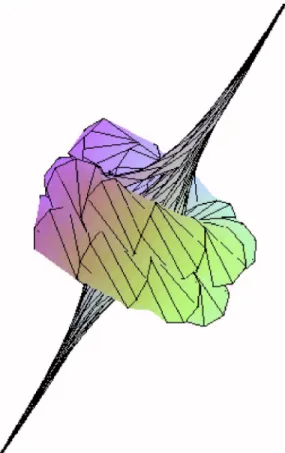
Example 2: By taking k1= 2 ,=1, and= −8 in Eqs.共44兲–共46兲, we get the surface 共Fig.1兲.
y1= − E1− 8/共e2+ 1兲, y2= − 4 cos G sech, y3= − 4 sin G sech, 共56兲
where E1= 4共x+3t兲,G=x+3t, and = x + t. As tends to ±⬁, y1 approaches ±⬁, and y2 and y3 approach zero. This can also be seen in Fig. 1. For small values of x and t, the surface has a twisted shape.
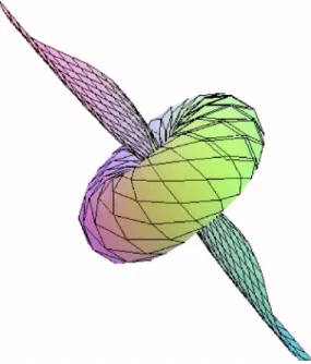
Example 3: By taking k1= 2,=0, and= −4 in Eqs.共44兲–共46兲, we get the surface共Fig.2兲.
The components of the position vector of the surface are
y1= − E1− 8/共e2+ 1兲, y2= − 4 cos G sech, y3= − 4 sin G sech, 共57兲
where E1= 2共x+3t兲, G=t, and= x + t. Astends to ±⬁, y1approaches ±⬁, and y2and y3tend to zero. This can also be seen in Fig.2. Asymptotically, this surface and the surface given in Example 2 are the same. However, for small values of x and t, they are different.
FIG. 1. 共x,t兲苸关−3,3兴⫻关−3,3兴.
Example 4: By taking k1= 3,=1/10, and= −452/ 75 in Eqs.共44兲–共46兲, we get the surface
共Fig.3兲. The components of the position vector of the surface are
y1= − E1− 8/共e2+ 1兲, y2= − 4 cos G sech, y3= − 4 sin G sech, 共58兲
where E1= −共5537t+2260x兲/750, G=17共497t+20x兲/200, and =共12x+27t兲/8. Asymptotically,
this surface is similar to the previous two surfaces. For small values of x and t, the surface looks like a shell.
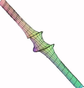
Example 5: By taking k1= 1,=−1/10, and= −52/ 25 in Eqs.共44兲–共46兲, we get the surface
共Fig.4兲. The components of the position vector of the surface are
y1= − E1− 8/共e2+ 1兲, y2= − 4 cos G sech, y3= − 4 sin G sech, 共59兲
where E1= −13共20x+t兲/250, G=共47t−20x兲/200, and=共4x+t兲/8. Asymptotically, this surface is similar to the previous three surfaces.
III. mKdV SURFACES FROM SPECTRAL-GAUGE DEFORMATIONS
In this section, we find surfaces arising from a combination of the spectral and gauge defor-mations of the Lax pair for the mKdV equation.
Proposition 5: Let u satisfy (which describes a traveling mKdV wave) Eq. (2). The corre-sponding su(2) valued Lax pair U and V of the mKdV equation are given by Eqs. (3) and (4), respectively. The su(2) valued matrices A and B are
A = i
冉
共
12−u
兲
−− −
共
21−u兲
冊
, 共60兲B = i
冉
1 2共␣+ 2兲 −共␣+兲u − 1 2u +共
1 2u2−␣−␣ − 2兲
−12u +共
12u2−␣−␣ − 2兲
− 12共␣+ 2兲 +共␣+兲u冊
, 共61兲where A =U+关2, U兴, B=V+关2, V兴, is the spectral parameter,and are constants, and2is the Pauli sigma matrix. The surface S , generated by U, V, A, and B, has the following first and second fundamental forms共j,k=1,2兲:
共dsI兲2= gjkdxjdxk, 共62兲 共dsII兲2= hjkdxjdxk, 共63兲 where g11=1 4 2+共关u2+2兴 −u兲, 共64兲 g12=1 4共␣+ 2兲 2+1 4共关2共 + 2␣兲u 2+ 4共3+␣ + 2␣兲兴 − 4共␣+兲u兲, 共65兲 g22= 1 4共u 2+共2 +␣兲2兲2+
冉
冋
1 4u 4+␣共␣− 1 +兲u2+共共1 + 兲␣+2兲2册
−1 2u 3−共␣2+共2 − 1兲␣+2兲u冊
, 共66兲 h11= 1 2u −共u 2+2兲, 共67兲 FIG. 4. 共x,t兲苸关−20,20兴⫻关−20,20兴.h12= 1 2共␣+兲u −
冉
共 2+␣ +␣兲 +1 2共 + 2␣兲u 2冊
, 共68兲 h22=1 4共u 3+ 2关␣2+共2 − 1兲␣+2兴u兲 −冉
1 4u 4+␣共␣− 1 +兲u2+共共1 + 兲␣+2兲2冊
, 共69兲and the corresponding Gaussian and mean curvatures are
K = 2u共u 2− 2␣兲 共2u关u2− 2␣兴 − 3u2− 2共2−␣兲兲 +2u, 共70兲 H = 共3u 2+ 2共2−␣兲兲 − 4u共u2− 2␣兲 2共2u关u2− 2␣兴 − 3u2− 2共2−␣兲兲 + 22u, 共71兲 where x1= x and x2= t.
A. The parametrized form of the four parameter family of mKdV surfaces
We apply the same technique that we used in Sec. II to find the position vector of the corresponding surface. Let u = k1sech,= k1共k12t + 4x兲/8, be the one soliton solution of the mKdV
equation, where␣= k12/ 4. The Lax pair U and V are given by Eqs.共3兲and共4兲, respectively, which is the same as in the spectral deformation case. So we can use the solution of the Lax equation 关Eq. 共5兲兴 that we found in the spectral deformation case. By solving Eq. 共10兲, we obtain the position vector, where the components of ⌽ are given by Eqs.共40兲–共43兲and A, B are given by Eqs.共60兲and共61兲, respectively. Here we choose A1= A2, B1=共A1e/k1兲/k1, and B2= −B1to write F in the form F = i共1y1+2y2+3y3兲. Hence we obtain a four parameter 共,k1,,兲 family of
surfaces parametrized by y1= R2 e2− 1 共e2+ 1兲sech+ R3E˜ + R4 1 e2+ 1, y2=
冋
1 2R4sech+ R5 共e4+ 1兲共e2+ 1兲2− R6sech2
册
cos G + R7共e2− 1兲 共e2+ 1兲sin G, 共72兲 y3=
冋
− 1 2R4sech− R5 共e4+ 1兲共e2+ 1兲2+ R6sech2
册
sin G + R7共e2− 1兲 共e2+ 1兲cos G, where R2= 2k1 2 k12+ 42, R3= 8, 共73兲 R4= 4k12 k12+ 42, R5= 共k12− 42兲 k12+ 42 , 共74兲 R6= 共42+ 3k 1 2兲 2共k12+ 42兲 , R7= 4k1 2 k12+ 42 , 共75兲
G = t
冉
2+1 4k1 2关1 + 兴冊
+ x, 共76兲 E ˜ = 共t关8 + k12兴 + 4x兲, 共77兲 =k1 3 8冉
t + 4x k12冊
. 共78兲Thus the position vector y =共y1共x,t兲,y2共x,t兲,y3共x,t兲兲 of the surface is given by Eq. 共72兲. This
surface has the following first and second fundamental forms共j,k=1,2兲:
共dsI兲2= gjkdxjdxk, 共79兲 共dsII兲2= hjkdxjdxk, 共80兲 where g11= 1 4 2+共关k 1 2 sech2+2兴 −k1sech兲, g12= 1 4共␣+ 2兲 2+1 4共关2k1 2共 + 2␣兲sech2+共43+ 4␣ + 42␣兲兴 − 4共␣+兲k 1sech兲, g22= 1 4共k1 2 sech2+共2 +␣兲2兲2+
冉
冋
1 4k1 4 sech4+␣k12共␣− 1 +兲sech2+共共1 + 兲␣+2兲2册
−1 2k1 3 sech3−k1共␣2+共2 − 1兲␣+2兲sech冊
, h11= 1 2k1sech−共k1 2 sech2+2兲, h12= 1 2共␣+兲k1sech−冉
共 2+␣ +␣兲 +1 2k1 2共 + 2␣兲sech2冊
, h22= 1 4共k1 3 sech3+ 2k12关␣2+共2 − 1兲␣+2兴sech2兲 −冉
1 4k1 4sech4+␣k 1 2共␣− 1 +兲sech2+共共1 + 兲␣+2兲2冊
,and the corresponding Gaussian and mean curvatures are
K = 2k1sech共k1 2 sech2− 2␣兲 共2k1sech关k21sech2− 2␣兴 − 3k 1 2sech2− 2共2−␣兲兲 +2k 1sech , H = 共3k1 2sech2+ 2共2−␣兲兲 − 4k 1sech共k12sech2− 2␣兲
2共2k1sech关k12sech2− 2␣兴 − 3k12sech2− 2共2−␣兲兲 + 22k1sech
, where x1= x , x2= t, and␣=1
4k1 2.
B. The analyses of the four parameter family of surfaces
Asymptotically, y1 approaches ±⬁, y2 approaches R5cos G ± R7sin G, and y3 approaches
−R5sin G ± R7cos G astends to ±⬁. For some small intervals of x and t, we plot some of the
four parameter family of surfaces for some special values of the parameters k1,,, andin Figs. 5–7.
Example 6: By taking k1= 2,=0,= −4, and = 1 in Eq.共72兲, we get the surface共Fig.5兲.
The components of the position vector are
y1= 2 sech共e2− 1兲/共e2+ 1兲 − E2− 8/共e2+ 1兲, 共81兲
y2=关− 4 sech+共e4+ 1兲/共e2+ 1兲2−共3/2兲sech2兴cos G, 共82兲 y3=关4 sech−共e4+ 1兲/共e2+ 1兲2+共3/2兲sech2兴sin G, 共83兲
where E2= −2共x+t兲,G=t and= x + t. Astends to ±⬁, y1 approaches ±⬁, y2 approaches cos t,
and y3approaches −sin t.
Example 7: By taking k1= 2 , =1,= 1 / 10, and= 1 in Eq.共72兲, we get the surface共Fig.6兲.
The components of the position vector are
y1= sech共e2− 1兲/共e2+ 1兲 + E2+ 1/共10共e2+ 1兲兲, 共84兲 y2=关共1/20兲sech− sech2兴cos G + sin G共e2− 1兲/共e2+ 1兲, 共85兲 y3=关− 共1/20兲sech+ sech2兴sin G + cos G共e2− 1兲/共e2+ 1兲, 共86兲
where E2=共x+3t兲/20, G=共x+3t兲, and = x + t. Astends to ±⬁, y1 tends to ±⬁, y2 approaches
sin共x+3t兲, and y3 approaches cos共x+3t兲.
Example 8: By taking k1= 1,=−1/10,= −52/ 25, and= −1 in Eq.共72兲, we get the surface 共Fig.7兲. The components of the position vector are
y1= −共25/13兲sech共e2− 1兲/共e2+ 1兲 − E2− 8/共e2+ 1兲, 共87兲
y2=关− 4 sech−共12/13兲共e4+ 1兲/共e2+ 1兲2+共19/13兲sech2兴cos G
+共5/13兲sin G共e2− 1兲/共e2+ 1兲, 共88兲
y3=关4 sech+共12/13兲共e4+ 1兲/共e2+ 1兲2−共19/13兲sech2兴sin G + 共5/13兲cos G共e2− 1兲/共e2+ 1兲,
共89兲 where E2= 13共20x+t兲/250, G=共47t−20x兲/200, and=共4x+t兲/8. As tends to ±⬁, y1 tends to ±⬁, y2approaches cos t, and y3 approaches −sin t.
IV. CONCLUSION
In this work, we considered mKdV 2-surfaces by using two deformations, spectral deforma-tion and a combinadeforma-tion of gauge and spectral deformadeforma-tions of mKdV equadeforma-tion and its Lax pair. We found the first and second fundamental forms, and the Gaussian and mean curvatures of the
FIG. 6. 共x,t兲苸关−6,6兴⫻关−6,6兴.
corresponding surfaces. By solving the Lax equation for a given solution of the mKdV equation and the corresponding Lax pair, we also found position vectors of these surfaces.
The surfaces arising from the spectral deformation are Weingarten and Willmore-like surfaces. We also obtained some mKdV surfaces from the variational principle for the Lagrange function, that is, a polynomial of the Gaussian and mean curvatures of the surfaces corresponding to the spectral deformations of the Lax pair of the mKdV equation. For some special values of param-eters, we plotted these three parameter family of surfaces in Examples 2—5.
In the case of the gauge-spectral parameter deformations, we obtained a four parameter family of mKdV surfaces. For some special values of the parameters in the position vectors关Eq.共72兲兴 of these surfaces, we plotted them in Examples 6—8.
ACKNOWLEDGMENTS
I would like to thank Metin Gürses for his continuous help in this work. I would also like to thank B. Özgür Sarıoğlu for his critical reading of the manuscript. This work is partially supported by the Scientific and Technological Research Council of Turkey.
1A. Sym, Lett. Nuovo Cimento Soc. Ital. Fis. 33, 394共1982兲.
2A. Sym, in Geometrical Aspects of the Einstein Equations and Integrable Systems, Lecture Notes in Physics Vol. 239,
edited by R. Martini共Springer, Berlin, 1985兲, p. 154.
3A. S. Fokas and I. M. Gelfand, Commun. Math. Phys. 177, 203共1996兲.
4A. S. Fokas, I. M. Gelfand, F. Finkel, and Q. M. Liu, Selecta Math., New Ser. 6, 347共2000兲. 5Ö. Ceyhan, A. S. Fokas, and M. Gürses, J. Math. Phys. 41, 2251共2000兲.
6M. Gürses, J. Nonlinear Math. Phys. 9, 59共2002兲.
7M. Gürses and S. Tek, Report No. nlin.SI/0511049共unpublished兲. 8B. G. Konopelchenko, Phys. Lett. A 183, 153共1993兲.
9B. G. Konopelchenko and I. A. Taimanov, Report No. dg-ga/9506011共unpublished兲. 10J. Cieslinski, P. Goldstein, and A. Sym, Phys. Lett. A 205, 37共1995兲.
11J. Cieslinski, J. Math. Phys. 38, 4255共1997兲.
12M. P. Do Carmo, Differential Geometry of Curves and Surfaces共Prentice-Hall, Englewood Cliffs, NJ, 1976兲. 13Z. C. Tu and Z. C. Ou-Yang, J. Phys. A 37, 11407共2004兲.
14Z. C. Tu and Z. C. Ou-Yang, Phys. Rev. E 68, 061915共2003兲.
15Z. C. Ou-Yang, J. Liu, and Y. Xie, Geometric Methods in the Elastic Theory of Membranes in Liquid Crystal Phases
共World Scientific, Singapore, 1999兲.
16Z. C. Tu and Z. C. Ou-Yang, Proceeding of the Seventh International Conference on Geometry, Integrability and
Quantization, Varna, Bulgaria, 2005, edited by I. M. Mladenov and M. de León, SOFTEX, Sofia, 2005, p. 237, Report No. math-ph/0506055.
17T. J. Willmore, Total Curvature in Riemannian Geometry共Wiley, New York, 1982兲.
18T. J. Willmore, Annals of Global Analysis and Geometry共Springer, New York, 2000兲, Vol. 18, pp. 255–264. 19Z. C. Ou-Yang and W. Helfrich, Phys. Rev. Lett. 59, 2486共1987兲.
20Z. C. Ou-Yang and W. Helfrich, Phys. Rev. A 39, 5280共1989兲. 21I. M. Mladenov, Eur. Phys. J. B 29, 327共2002兲.