A hypergraph-partitioning based remapping model for image-space parallel volume rendering

(1)

,іВ ' il S i H i

'i ?<:

Г

28S

^ с ж

(2)

A H Y P E R G R A P H -P A R T IT IO N IN G

BASED R E M A P P IN G M O D EL FOR

IM A G E -SP A C E PARALLEL

V O L U M E R E N D E R IN G

A THESIS

SUBMITTED TO THE DEPARTMENT OF COMPUTER ENGINEERING

AND THE INSTITUTE OF ENGINEERING AND SCIENCE OF BILKENT UNIVERSITY

IN PARTIAL FULFILLMENT OF THE REQUIREMENTS FOR THE DEGREE OF

MASTER OF SCIENCE

l)y

B e r k a iit B a i i a C a m b a z o g lu F o l)r u a iy ,

2000

(3)

T З Ь '

•съа

,ζίοοο

(4)

I certify that I have read tliis thesis and that in my opinion it is fully adequate, in scope and in quality, as a thesis for the degree of Master of Science.

As.soc. Prof. Cev(/et Aykanat (Advisor)

I certify that I have read this thesis and that in my opinion it is fully adequate, in scope and in (luality, as a thesis for the degree of Master of Science.

I certify that I have read this thesis and that in my opinion it is fully adeciuate, in scope and in (|uality, as a thesis lor the degree of Master of Scicnice.

roI'LAtilla Giii soy

Approved for the Institute of Engineering and Science:

Prof. Melmiet Da;

Director of Institute of Engine^'ing and Science

(5)

A B S T R A C T

A IIYPERG RAPII-PAR'rrnON IN G BASED REMAPPING MODEL FOR IMAGE-SPACE PARALLEL VOLUME RENDERING

Berkaiit Bcirla Cambazoglu M.S. in Computer Engineering Supervisor: Assoc. Prof. Cevclet Aykanat

February, 2000

Ray-casting is a popular direct volume rendering teclinique, used to explore the content of .'ID data. Although tliis teclmique is capable of producing high quality visualizcvtions, its slowness prevents the interactive use. The major method to overcome this speed limitation is parallelization. In this work, we investigate the image-space parallelization of ray-casting for distributed mem ory architectures, d'lie most important issues in image-space parallelization are load balancing and minimization of the data redistribution overhead introduced at successive visualization instances. Load balancing in volume rendering re- ((uires the estimation of screen work load correctly. For this purj^ose, we tested three diiferent load assignment schemes. .Since the data u.sed in this work is made up of unstructured tetrahedral grids, clusters of data were used instead of individual cells, for eiliciency ])urposes. Two diiferent cluster-proces.sor di.s- tribution schemes are emi)lo3'cd to see the effects of initial data distribution. The major contribution of the thesis comes at the hypergraph pcirtitioning model proposed as a.solution to the renurpping problem. For this purpose, ex isting hy))ergraph partitioning tool PaToII is modified and u.sed as a one-phase remapiiing tool. The model is tested on a Pcirsytec CC system and satisfactory results are obtained. Compared to the two-phase jagged partitioning model, our work incurs less preprocessing overhead. At comparable load imba.la.nce values, our hyiiergraiih partitioning model requires 25% less total volume of communication than jagged partitioning on the average.

K e y w o rd s: image-space parallelization, ra.y-casting, unstructured grids, work load assignment, hypergraph partitioning, load balancing, remapping.

(6)

ÖZET

GÖRÜNTÜ-UZAYI PARALEL HACİM GÖRÜNTÜLEME İÇİN IlİPERÇİZGE BÖLÜMLEMEYE DAYALI YENİDEN EŞLEME MODELİ

Berkant Barla Cambazoğlu Bilgisayar Mühendisliği, Yüksek Lisans Tez Yöneticisi: Doç Dr. Cevdet Aykanat

Şubat, 2000

Işın izleme, üç boyutlu verilerin incelenmesinde kullanılan, popüler bir doğ rudan hacim görüntüleme tekniğidir. Bu teknik yüksek kalitede görüntüler üretebilecek kapasitede olmasına rağmen yavaşlığı birebir etkileşimli kulla nımını engellemektedir. Bu hız sınırlamasını cişmanın en önemli yolu pa ralelleştirmedir. Bu çalışmada, ışın izlemenin dağıtık bellekli mimarilerdeki görüntü-Lizayı paralelleştirmesi araştırılmıştır. Görüntü-uzayı paralelleştirme deki en önemli konular yük dengeleme ve takip eden görüntüleme örneklerinde ortaya çıkan veri yeniden dağıtım yükünün en aza indirilmesidir. Hacim gö rüntülemedeki yük dengeleme, ekran iş yükünün doğru olarak talıminini gerek tirmektedir. Bu amaçla, üç değişik yük tahsis etme planı denenmiştir. Bu çalışmada kullanılan veriler düzensiz tetrahedral ızgaralardan oluştuğu için, verimlilik amacıyla bireysel veri hücreleri yerine veri grupları kullanılmıştır, ilk veri (lağılımınnı etkilerini görmek için iki farklı veri grubu-işlemci dağılım pla.nı kullanılmıştır. Çalışmanın en önemli katkısı yeniden eşleme problemi ne bir çözüm olarak önerilen hiperçizge bölümleme modelidir. Bu amaçla, var olan hiperçizge ])arçalama aracı PaToH değiştirilerek tek Scifhalı yeniden eşleme aracı olarak kullanılmıştır. Model Parsytec CC sisteminde denenmiş ve tatmin edici sonuçlar elde edilmiştir. Önerilen yöntem iki sal'hah kesikli bölümleme modeline göre, daha az ön hazırlık yükü yaratmaktadır. Kıyaslanabilir yük dengesizliklerinde, önerilen hiperçizge modeli kesikli bölümleme modelinden ortalama %25 daha az toplam iletişim hacmi gerektirmektedir.

A n a h ta r K elim eler: görüntü-uzayı paralelleştirme, ışın izleme, düzensiz ız garalar, iş yükü tahsisi, hiperçizge bölümleme, yük dengeleme, yeniden eşleme.

(7)

ACKNOWLEDGMENTS

I thank to my advisor Assoc. Prof. Cevdet Aykanat for his ideas, suggestions and help on this thesis. I also tliank Asst. Prof. Uğur Güdükbciy and Asst. Prof. Atilla Giirsoy for reading thesis. I express my endless thanks to my family and my friend Ayça Ozger for their support and patience.

(8)

List of Figures

J.l Grid types in 2D... 2

1.2 llendering pij)elincs for distributed memory architectures... 5

2.1 Ray casting. 10

2.2 Ray-casting for rnid-point sampling. . . 12

2..'1 l);rta. structures for tetrahedrivl unstructured data. 12

2.1 A Ccise wliere face soi tiiig fails... 1.3

2.5 Ray bufTers contain the ray-segments generated for each [)ixel. . 14

2.0 Intersection test.

2.7 l·bκam|)le transfer functions. 17

3.1 l)a.ta.-pi'ocessor assignments in OS and IS parallelization...21

3.2 (Jell clusterizati 23

3.3 Atlditioiial data structures used after clusterization. 26

3.4 ScrecMi subdivision teclmic|ues... 27

3.5 Effect of projection area on grid granularity... 28

3.6 Work load assignment schemes... 31

(12)

4.1 Multilevel liyi^ergrai)!) bisection... 37

5.1 Representing the interaction between OS and IS by an hypergraph. 41

5.2 The partitioning cost calculated by two-phase method may be

incorrect. 43

5.3 Special vertices are introduced into the hypergraph in one-plmse model... 44

5.4 Cluster distribution schemes... 46

5.5 K.endiired image of CC data set... 49

5.6 Example region-processor assignment in jagged partitioning. . . 50

5.7 Example region-processor assignment in hypergraph partitioning. 51

7.1 Load iinba.lances i a IIP and JP... 66

7.2 ]^-e|)i-oces.sing overhead incurred in HP and JP. 67

7.J A compcirison of conmiunication volumes in HP and JP... 68

(13)

List of Tables

1.1 Grid classification. 2

1.2 Pa.i‘alldizatioii of DVR. algortiliins. 6

3.1 Possible weighting schemes for the clusterization graph... 24

7.1 Some features of the data sets used... 58

7.2 Al)l)r(wiatioiis used in tables... 59

7.3 [{esults ol)tained l)y assigning different cluster counts per |)ro-cessor... 60

7.4 Effects of all possible weighting schemes used in the clusteriza tion graph... 60

7.5 lifleets of diffei’ent work load calcuhition schemes... 61

7.6 Iml)alance values cuid communication ermounts ol)served. 62

7.7 Dissection of view dependent preprocessing time. 63

7.8 Si)eedup cuid efficienc}^ values for different data sets and proces sor numbers... 64

A .l Adaptive granularity calcuhition. 78

(14)

List of Symbols and Abbreviations

DVR ISP OSP IIP JP II h f ejj ebf KL PM a, /i/, 7 R. Gi B, O, A. % ■^('ir ./■ Area{f) N Ttr lir l\c Gc Gy Th tit T_vs trs T

: Direct, Volume Rendering. Image-Space Parallelization. 0 1) ject-Sj)ace ParalIcl ization. Il.ypergra.pli Partitioning Jagged Partitioning front-facing,

back-facing,

external front-fadng. <;x t<M' n a.l 1) ack - fa(;i n g.

Kernighan-Lin liypergrapli partitioning heuristic. Fiduccia-Mattheyses hypergrapli partitioning heuristic. Scaling coefRcients in intersection test.

Red color component of ¿tli resampling point. Gi'(;en color component of ¿th resamj)ling point. Blue color component of ¿th resampling point. Opacity component of ¿th resampling point. Transfer function for component ;c, where x G Set of .//■faces.

Set, of eJJ faces. A tetrahedral face.

l''unction which returns the area of lace ,/. Number of nodes in the data.

Total time spent on node transformation. Average time s]>ent to transform a single node, dotal time spent on scan conversion of Cj//’ faces. Avei age scan convcnsion cost for a. |)ixel.

Number of intersections made by a ra.y shot from pixel {x ,y )· Total time spent on intersection test.

Average time spent on intersection test for an intersection. Total time spent on resami)ling.

Average resampling time of a point, dotal time s])ent on rendering.

(15)

G V £ Vi Cij 'Wi U)K!

c

Ci

s

Si ■>'i K P P' Pi n n ' V V M Vi n-i Pi IT IT' e li'v) lfr{v) Bp,{n) M{S.) <h Si

Craph used in clusterization. Set of vertices in G-

Set of e<lges in G- itli vertex in set V.

Edge connecting vertices Vi and vj. Weight of the vertex v¡ in set V.

W<'ight of the edge between vertices u,· and vj. Set of data dusters.

•¿th cluster in set C.

Set of screen parts, ith screen part in set S.

¿th screen cell.

Number of processors used. Set of processors used.

Set of processors to which a cluster will migrate. ¿th processor in set P.

Remapping hy])ergraph in two-phase model. Remapping hy|)(Mgraph in one-phase nuxlel. Sc;t of vei'tices in 'H.

Set of vertices in 'H'. Set of nets in "W.

¿th vertex in a hj'pergraph. ¿th net in a. hypergra.])h.

¿th special vertex, representing Pi in 7i'.

Set of screen parts returned by hypergraph partitioning in two-phase model. Set of screen parts returned by hypergraph partitioning in one-phase model. Overall load imbalance value for a partition.

Set of exteriud nets which has a pin on a vertex in set V'. Gain obtained by moving vertex v.

?-th level Gain obtained by moving vertex v. Binding number ol net n.

Mapping función vvliich maps <5,· to Pj.

Degree of ¿th vertex in a hypergraph. Size of ¿th net in a hypergraph.

(16)

\i , \ ( n ) Pins{iii,) Ntts{'Vi) B X

y

z

Xi Vi Load{Ci) L()ad{vi) C ost[e,)

: Connectivity set of a net iii. Connectivity of a net iii. Cost of the partition II.

Operator which returns the set of vertices on wliicli ni has a pin. Operator which returns the set of nets which has a pin attached on vi Bipartite grapli used in the second phase of two-plnise model.

Set of i)rocessors in B. Set of screen parts in B. Set of edges in B.

vertex representing zth processor, in set X . vertex representing zth screen part, in set 3^.

Function tliat returns the rendering load of the cluster C,·. Fimction that returns the rendering load of the screen cell vi. Function that returns the migration cost of the cluster C{,

(17)

Chapter 1 Introduction

The huge im])rovements in computing capa))iliLies of luuxlware, and develop ments on the visiuilization software allowed researchers, students and people from many different work areas to study the interiors of 3-dimensional data on their desktops. 'IcKhiy, volume visualizaiion stands as a. scicmce disci|)line, which is commonly used as a. tool to aid the research b}' letting the scientists to get a. visual grasp of the problem under investiga.tion. d’he main method for scientific volume visualization [36] is volume rendering. Tt finds applica tion in various areas such as hydrodynamics, molecular biology, sysmology and nu'ti'orology.

1.1 Terminology and Classification

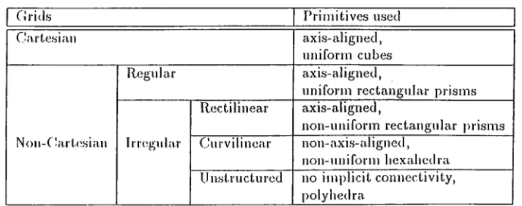
Volume rendering can be simply defined as the process of mapping a set of scalar, tensor or vector values defined in 3D to a 2D image screen. In order to iei)reseut these volumetric data sets, clifTerent kinds of grids are used. Grids, according to their structural properties, can be classified as in Table 1.1.

Irregular grids are the most interesting type of grids with the cvbility to rep resent dis|)a.rate field data effectively. In rectilinear grids, non-unilbrm, axis- aligned rectangular prisms arc used as volumetric primitives (voxels). Curvilin ear grids have the same topological structure with rectilinecir grids, but they are

(18)

c u AFTER í. INTRODUCTION

Table 1.1. Grid classification.

G rids Primitives used

CJ artesian ax is-aligned,

uniform cubes

Non-C!art(^sian

Regular axis-aligned,

uniform rectangular prisms

irregular

Rectilinear axis-aligned,

non-uniform rectangular prisms Curvilinear non-axis-aligned,

non-uniform hexahedra Unstructured no implicit connectivity,

polyhedra

warped from computational space to physical space. With the increase in the number of tools and methods for generating high qucility adaptive meshes, un structured grids are also gaining more popularity. Unstructured grids contain polyhedra with no implicit connectivity infornuition. Volumetric primitives {cells) such as tetrahedra, hexaliedra, and prisms can be used in these grids. However, because any volume can be decomposed into tetrahedra, and they are easy to work with, in most cases tetrahedral cells are used to form unstructured grids. IHgure 1.1 shows 21) ecjuivalcnts of these grid types.

Carlcsian Regular Rcclilinear

Figure 1.1. Grid types in 2D.

d"wo basic categories can be considered for volume rendering algorithms [7]: Surface-based algorithms, whicli compute different levels of surfaces within a given volume, and direct volume rendering (DVR) algorithms, which display the integral densities along imaginary rays passed between the viewers eyes and the volume data. Surface based metliods are sometimes referred as indirect methods, since they try to extract an intermediate representation for the data set. Their mciin idea is to construct some level surfaces using the sample points with close density values, and represent them with a set of contiguous polygons, which will later be rendered in the standard graphics pipeline.

(19)

CIIAPTEli I. INTRODUCTION

Dc.s|)ile l,lic fact that surrac(;-I)ivsed algorithms arc fairly well suited for areas such as medical imaging, which requires specific tissue boundaries to be dis|)la.ycd, there are many other areas in which they cannot be utilized due to the problems associated with the computation of surface levels. In most data, sets, using artificial surfaces may result in highly non-linear discontinuities in the data and introduces artifacts in the rendered image. In other words, a sui'lace may not always rei)res(Mit the actual data structure correctly. To overcome this problem, direct volume rendering technicpies, which treat the volume data as a. whole, are emplo3^ed. DVR is a powerful tool for visualizing data, sets with complex structures defined on 3D grids.

The main DVR methods are ray-casting and data projection, which are sometimes referred as image-space a.nd object-space methods, respectively. Cell projection [12] and splatting [45] are the two examples of object-space methods. In cell piojection based DVR algoritlirns, the projection primitives (tricvngle, tetrahedra, or cube) must be sorted with respect to the viewing point, due to the usage ol tin; com|)osition lormula. based on color and opacity a.ccumulation at sam|)liug points. However, because of the ambiguities in the visibility or dering [12] of projection primitives, the visualization process may yield a poor final rendering. Similar problems, which affect the image qualitjq arise in other object-spacc! methods, too. For example, in splatting algorithms, efl'ect extends of the rc'sa.mpling points should be approximated correctly.

Ra.,y-ca.sting [18, II], without anj' luisitation, can be said to be a very good candidate to produce high-quality, realistic images. This method works by shooting rays from the image ])lane into the volume data, and combining the color and opacity values calculated at resampling points throughout the data. Because ea.ch ray’s contribution to a pixel color is independent of all other ra.ys, ray-casting algorithms cannot utilize the object-space coherency well. As a. result, their elegancy comes at a cost.

The computational cost of DVR algorithms is affected by the huge amount of information to I)e processed in the data sets, and it prevents their wide- spread use. Although many optimization techniques cue known, speeds of DVR algorithms are still far from interactive response times. The CPU speeds at which the current |)rocessors operate is not the only limitation before direct

(20)

CIÎAPTEH L INTRODUCTION

volumes r(3Ji(leiTng. Limited amoımt of ph^^siccil meınoıy in workstiitioiis can filso be a lx)Ul(3neck. Since some portions of the datci may not fit into main memory, it may be necessciry to access the data fi*om virtual mejriory resulting in a much slower data ciccess I’ate.

Parcdlelization of the existing DVR algorithms [46] is the main technique to ov(3rcome tlie sjxied limitations mentioned above. Considerable speedups can be gained through parallelization without trading the image quality for render ing speed. Shared memory or distributed memory architectures can be used for parallelization. In shared memory parallel machines, ecich processor has access to a global memory via some interconnect or bus. The globed memory can b(3 a singl(3 module, or can l)e divided equally among processors. Processors communicate by using the bus, through read and write operations performed over memory locations in the global memory. Although it presents ease of ])rogramming and flexildlity, shared memory architectures does not scale well, due to the bottlenecks occurred during memory access.

In distributed memory ¿irchitectures, each processor is given its own mem ory, which is not directly accessible by other processors. If a processor needs data contained in the mejiioiy ol a remote processor, it sends ¿1 message ¿isking for the data and reti'ieves it Irom that processor through an interconnection network. As a result, the data access is not always uniform, ¿ind issues such as data distribution, coimnunication bcindwidth and network toi)ology gain im|)ortance.

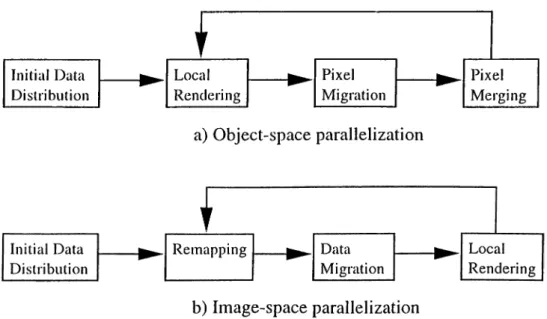
Parall(4ization process can be carried out in 3D object domaiji or 2D screen domain, r(3sulting in object-space parallelization (OSP) and image space paral lelization (ISP), respectively. In OSP, each processor is assigned a sub-volume of the data, and produces the partial color information for the final image by rendering its volumetric primitives. Ltvter, these partied results ¿ire merged ¿it ¿ippropriate processors by a pixel merging step. Communication is needed to send the sub-results to their destination processors, where they will be com bined to determine the iimil pixel colors. Hence, OSP is known ¿is a pixel-flow nudJiod.

(21)

an A PTim i

. i n t i i o d

i

k j t i o n

f

Initial Data Local Pixel Pixel Distribution Rendering Migration Merging

a) Object-space parallelization

b) Image-space parallelization

Figure 1.2. Rendering pipelines for distributed memory arcliitectures.

each processor is assigned a sub-region over the screen and is res])onsible for rendering that particular region. However, since a processor may not possess all the primitives necessary lor rendering its region, required sub-volumes £i.re retrieved Irom |)iocessors owning them, before the rendering process starts. I'^igure 1.2 dis|)lays the general rendering pipelines for OSP and ISP on dis tributed uKiinory arcliitectures.

1.2 Previous Work

With the increase in their availability and decrease in their prices, massively |)arallel computers a.ie becoming more popular. In the last decade, many at tempts were done to parallelize the existing DVR. a.lgorithms. However, most of these work dealt with the structured kind of data. Work on unstructured data took less attention. 'Γ¿d)le 1.2 displays the references to latest work on paral lelization of DVR methods. The classification in that table is done according to the type of the architecture and the parallelization method used.

Although lots of research is carried out on volume visualization, it is still very diificult to establish the standards to compare the quality of the works done on volume rendering. Unfortunately, this becomes more apparent in

(22)

c n AFTER. 1. INTRODUCTION la b le 1.2. Panil]elizcition of DVR algortihins. OS Parallelization IS Pcirallelization Shared Memory

[

44

]

[

35

]

Distributed Memory 32

]

[

37

]

[

4

] [

29

]

Special Ilardwa 47

[

48

]

l)ara.llclization of DVR. methods, ddiere are rna.ny criteria such as data set size, execution speed, image quality, load balance, speedup, sccdability tliat can be used to cornpai'e work with the previous, similar works. This makes their COn 1 pari sou h aixler.

Considering the classification made in Section 1.1, our work can said to be the ))arallelization of ra.y-casting technique for distributed memory architec tures. In our work, image-space decomposition was chosen for parallelization and th(i data used is of ty|)e tetrahedral unstructured grids.

There is little research done in this iirea. Hence, we compared our work with a similar algorithm, which irses jagged ])c\.rtitioning to divide the screen. Ja.gged partitioning is one of the best screen space subdivision algorithms. However, since it is mainly concentrated on the load balance between partitions, it lacks the i)ower to minimize the communication between partitions. At same load ba.lance, and preproce.ssing overheads we observed that the communication cost during the remapping phase, incurred by ja.gged partitioning can be up to 30% higher than the cost observed in our work.

1.3 Proposed Work

The lay-casting code we used is a slightly modified implementation of Koya- mada’s ray-casting algorithm [26]. This algorithm is a rather efficient algo- I’ithm, which makes use of both object-spcice coherency and inicige-space co herency. Our main modification to this algorithm is the use of a higher level of volumetric data abstraction.

(23)

CHAPTER 1. INTRODUCTION

1 1 1 some cases, instead of working on individual tctraliedral cells we deal witli connected clusters of tetrahedral cells. Although introducing clusters may result in data reiilication during parallelization, this effect may be negligible if the number of clusters used is ke|)t high enough. Clusterization [9] simplifies the liousekeeping work, and decreases the number iterations in some loops. Its main use comes at the computation of the screen work load, i.e., the distribution of the cell liMidering costs over their ])rojection areas on the screen. In addition, this clusterization process is necessary to obtain the condensed hypergrai)h which will be used during the remapping step.

Tire fundamental problem in image-space based DVR metliods is that if a visualization parameter such as the viewpoint location or the viewing di rection changes, the image on the screen should be wholly recom])uted. For image-space parallelization, this creates a j:)roblem known cis the remapping problem. During successive visualizations, the rendering costs of volumetric primitives distributed over screen pixels can largely change, resulting in severe load imbalances among the procès,sors. 'Phis necessitates the rnigraXion of some volume data, to other processors in order to ba.la.nce the load distrilnition. The aim of remapping step is both to obtain a good load balance by shifting data from heavily loa.ded processors to lightly loaded processors, and to minimize the communication overhead incurred by this data migration.

Our main contribution is at the ])roposed remapping model. In this work, remapping problem is formulated as a. hypergraph partitioning problem, so that the interaction between the object and image domains is represented by an hypergraph. A net in this h3q)ergraph stands for a cell cluster in the volume data, and its weight shows the migration cost of the cluster. Cells of the h3'pei'gra.|)h represent the pixels over the screen. Each pixel’s rendering cost is assigned to its re])resentative cell.

'Pile tool used for hyi)ergra.ph partitioning is PaToII. In order to obtain a one-phase rema.pi)ing model, some modifications were done on the hypergraph model and PaToII, giving them the ability to treat some cells differently than the others. Some special cells are placed in the hypergraph to represent the ])rocessors used during execution. A special vertex is connected to a net by a pin, if net’s cluster resided in the local memory of the proces.sor. Details of

(24)

this oiie-pliase model can l)c found in Chapter 5.

Tlie iini)lementation of our parallel rciy-casting algorithm is composed of four consecutive phases: View independent preprocessing, view dependent pre- ])rocessing, cluster migration and I’endering. View independent preprocessing is performed just once at the beginning of each run. It includes some steps such as cell clusterization, initial data distribution, and disconnected cluster elim ination. In view dependent ])reprocessing, some transformations are applied on the data, and also clusters are mapped to new processors through hyper graph partitioning. In cluster migration step, communication is performed to send clusters to their new locations. An important fact is that the overhead incurred by these last two steps should be minimal, since they are executed at the beginning of every visualizcition instance. The final step is the rendering of the clusters locall}^ by the processors. Because processors have all the clusters needed over their assigned screen regions, no global pixel merging is necessary.

с п л т т 1.

intiioduction s

The organization ol the thesis is as follows: In Chapter 2, ray-casting ¿md our imphnueiitation of Koyamada’s algorithm were ex|)lained. Chapter 3 dis cusses image-space parallelization issues. Cluipter 4 is an introduction to hypergra])h partitioning. Our remapping model and parallel ray-Ccisting imple mentation were presented in Cliapter 5 and Chapter (i, respectively. Chapter 7 gives some experimental results, and Chapter 8 concludes the thesis.

(25)

Chapter 2 Ray-Casting

Ray-casting is an image-space rendering method, in which some rays are shot from the observers eye (vietopoinl) into the volume data through tlie pixels over the image screen, and fiiud pixel colors are calculated using the color contributions of the sa.mple points over the ray. Sometimes, in the literature, tlu! t('rm ray-casting is used to rcifer to ray-tracing, although they are not the same. In ray-casting, oidy the shadow rays are considered, ignoring reflection rays cUkI transmission rays which are important in ray-tra.cing. Tims, ray casting can lje said to be a simple form of traditional ray-tracing.

The next section describes the basic ray-casting algorithm. In the section following it, Koyamada’s ray-casting algorithm which works on unstructured grids is explained. This algorithm forms the basis for our ray-casting code. r<'inally, some optimizations done in ray-casting and the peiformance of our rendering algorithm is discussed.

2.1 Basic

R a y -

Casting Algorithm

Before the ray-casting algorithm has started, it is assumed that the scalar values on grid vertices and the vic.'wing orientation were already determined I)y the user. The viewing orientation is specified by the following three parameters: view-rcjcrence poini, view-direclion vector, and view-up vector, 'rogether with

(26)

CllAPTKli 2. RAY-CASTING 10

these thro;e parameters, image screen resolution parameter is used to transform the grid vertices, which are originally in world space coordínale (W SC) system, into normalized projeclion coordínale (NPC) system, which will be used in ray casting. Also, some transfer functions, which will map the scalar values at resampling points into an RGB color tuple and an opacity value, were assigned previously.

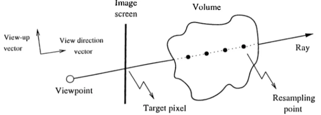
In ray-casting we perform an image-order traversal over the screen pixels, and try to assign a final color value to each pixel. To find a pixel’s color, first, a ray is shot from the viewpoint into the volume data passing through that pixel (Figure 2.1). This ray is followed within the volume, and some sample valiK.'s are calculated at the resampling points along the ray at some regular intervals. If the resampling point is not exactly on a grid vertex, its Vcilue is approximated by interpolating the scalar values at some close grid vertices. Different sampling methods and interpolation techniques are discussed in the following .sections, in more detail.

Image _Volume

Figure 2.1. Ray casting.

At each resampling point, tlie transfer functions are a]:>plied to the sample values found, and color and opacity contributions of resampling points are Ccdculated. Then, using a weigliting formula, these color and opacity values are accumulated into the final color value of the pixel, from which the ra.y was shot. The weighting formula is such that, the points closer to the pixel contribute more than the points far from the screen.

Tins sam[)ling step repeats until the ray reaches the end of the volume or the accumulated opacity reaches unity. At the end, the accumulated color tuple is multiplied by the partial opacity and the final color is stored for that

(27)

CIIAPTFJI 2. RAY-CASTING

pixel. The algoritlini continues by moving onto the next pixel, cincl performing ¿ill the steps ¿ibove for this newly selected pixel.

2.2 Data Structures for Unstructured Grids

(ii'ids rcprcsentiiig voliinicl.ric data can be conslructed from differenl primitives sucli as rectangvdar prisms, hexahedron, tetraliedron, polyhedron or a. mixture of these. As we did in this work, mostly tetrahedral primitives are used in unstnictured grids. We refer to tetrahedral volume elements as cells here. All types of polyhedra can he converted into a set of tetrahedral cells through a process called tetrahcdralization. A points value inside a. tetrahedral cell can be interpolated directly, and the data distribution is linear in any direction inside the cell. Also, for this type of cells explicit connectivity structure is easier to be establislied.

A cell is made up ol lour planar, triangular faces and four corner points, called its vcrliccs. liacli vertex o( a cell is actually a. sample point with WSC values cuid an associated scalar value. The cell faces a.re classified as either internal or external. A common lace shared by two different cells is an internal face. If a. face is not shared by a iieighbor cell, it is an external face. We call a cell with no exteriurl faces as an internal cell. Otherwise, the cell has a.t least one external face, and it is called an external cell.

(Jell laces can cilso be classified according to the angle between their normal vectors and the view direction vector. If tluxse vectors are perpendicular to each other, then the lace is parallel to the ray casted. In case the angle is less than 90", we call the face a front-facing (Jf) face. Otherwise, it is a back-facing (bf) face. An external .//face is named as an e//face. Similarly, an external. / / face is named as an ebf face. Finally, we use the sets iFfj and iFejj to denote the sets of .//and effa ce s, respectively (Figure 2.2).

Our tetrali('draJ c(dl data structure mainly contains two arrays: Nodes array, and Cells array. Size of the Nodes array is ecjual to the number of sampling points in the data. Each item of this array represents a single sampling point

(28)

CHAPTER 2. RAY-CASTING 12

l''igure 2.2. Ray-casting for unstructured grids with mid-point sampling.

and stores that points WSC, NPC values as well as the scalar va.lue iit that point. The scalar and coordinate values are stored as flocit numbers.

The second major array, namely the Cells array, is used to establish the connectivity l)(;tw('cn tin; cells, d'he number of items in this array equals to the tetiahedral cell count in the data.. In an arra.y item, for each face, the following information is stored: Nodes array indices of the four vertices forming the cell. Cells ariciy indices of the four neighl)or cells, and a number ra.nging fi’orn 0 to 3 to distinguish the shared faces of the neighbor cells. For non-shared faces of external cells a sentinel value of -1 is used. The data structures used can be seen in Figure 2.3. struct Node { struct Point WSC; struct Point NPC; float scalar; } struct Point { float x; float y; float z; } struct Cell { iiit vert ices [4]; int neigliborCells[4]; int neiglıbor^aces[4];

}

(29)

2.3 Koyamada’s Algorithm

Koyamada’s algorillun is a ray-casting algorithm that works on unstructured grids and is a ratlier efficient algorithm. It both tries to use the image-space coherency existing on the screen and the object-space coherency within the data. Image-s))ace coherency is ex])loited during the scan conversion of effinces, in order to determine the first ray-cell intersections. Object-space coherency is utilized by means of the connectivity information between the cells. Moreover, the residts obtained from ray-face intersection is used for interpolation of scalar values making the interpolation operation very fast. Finally, due to the linear sampling method used, the resampling operations are very efficient.

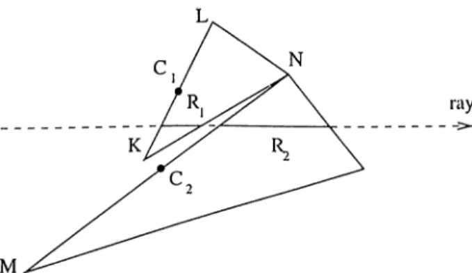
Initial step taken in tlie algorithm is to scan convert the ejj faces and find the first ra.y-volume intersections. Because the volume or the sub-volumes used during parallelization may be non-convex, more than one riiy-segment may be generated for the same ])ixel. Due to the nature of the color composition for mula., this ray-segments should be merged in a. sorted order. In the original algorithm, cj] fa.c<\s are sorted with respect to the 5: coordinate of their cen troids, and scan converted in that order.

However, this is an ai)proximate ordering and may be wrong in some cases as shown in Figure 2.4. In that figure, although Ri should be traversed before /¿2, II2 is proce.s.sed and composited first; since the centroid of K L , C*!, is sorted before the centroid of M¡V, C^· Our im])lcmentation overcomes this problem, which may lower the image quality, by means of a ra.y bufl’er data structure. This data structure keeps a linked list for each pixel, and the list elements

(30)

an A PTica 2.

ray

-

casting 14

contain composition infonnation (i.e. accnmnlated color and opacity) about the ra.y-segmcnts fired from that pixel (Figure 2.5). After all ray-segments

nrc; (’« ilrn la t(u l aiicl inwca tcjcl in to Uu^ir i'<\s[)(3c(.iv<i li.s(.H in Horl.iHl ordc.'r, a.m

mcrg(;d by a pixel merging ste]) in correct order.

Figure 2.5. Ray l;>uiFers contain the ray-segments generated for each pixel.

The ray segments are traversed until tliey exit at some point from an ebf face of the volume. When a ray enters a cell from a face it exits tl>e cell tlirough one ol that cells remaining three faces. This particulax exit face, and the exit point coordinates are iound by the intersection test. An exit point from a cell constitutes the entry j)oint to another cell, therefore just one intersection is performed per cell.

'I'he following snbsections discu.ss the two important steps of the algorithm, that is, the intersection test, and the resampling steps, which are performed in an interleaved manner.

2.3.1 Intersection Test

In Figure 2.6, we consider the intersection test of a ray with the A B C face of a cell. Since x and y coordiruites for the exit point Q are already known

— /2.,. and Qy = Ry)^ the problem is to find the coordinate value. This is done by expressing A(^ as the summation of the two vectors whose directions are same with AD and

(31)

Figure 2.6. Intersection test.

ller(i, fv and fi are tlie cociricients used for scaling. The e(|iiation al)ove can be rewritten in a inoie useiul matrix form as follows:

(2.2)

' B x - /1 , Cx- /u . 0 ■ a Rx _-Ax

B y - A y C y - A y 0 X = Ry - Ay

Bz - Az Cz - Az 0 _ _{. 7 .} . Qz - Az _

In Fquation 2.2, (/Ij,.,/ ! „ , /L )i (^i·, Gy, and {C x,C y,C z) represent the coordinate values of /1, D c\.nd C points, respectively. By solving the ecpiations in the first and second lines of Equation 2.2, unknown a and /3 coefTicients in h'quation 2.1 can be calcidated. If one of the cv > 0, /? > 0, and 1 — a — /3 < 0 conditions does not hold, then the ray does not intersect the face an another face is tested in the same marmei'. The 2 coordinate of the exit point Q can be calculated by sul)stituting the values found, into the Equation 2.3.

(32)

2.3.2 Resampling

Next step in tlie algorithm is to find the scalar value at the exit point. That value is ap])roximated by the inter])ola.tion of the scalar values at some sampling points. Koyamada’s algorithm employs 2D inverse distance interpolation to calculate the scalar Qs at point Q.In our example, the scalar values Л,, /?j, and at facci coriuM's /1, В and C are interpolated for tins purpose. Tlie cv and fi coefficients found during the intersection test is used in the following i n t e r p о 1 a t i о n fo r 1 rnd a:

Q a = c x D s + ¡ З С з + (1 — q; — (2.4)

Using (P,,Pa) and (Q^^Qs) tuples, new scalars are calculated within the cell, by ID inverse distance inter])ola.tion, along the ra.y segment bounded by the P entry, and the Q exit points. The number of resampling points depends on the method used. li(|uidistance sampling, adaptive sampling, and mid-point sampling are the most common resainpling methods.

In ec|uidista.nce sampling, the distance between successive resampling points is constant and scalars ai'e calculated by ID inverse distance interpolation using entry and exit points. Ada]:)tive sampling takes the cell size variation into consideration and determines a different resampling distance for each cell. In mid-point scimpling resampling is done at the middle of the ray-segment. The method used in this work is mid-point sampling. It is both fast, since the resa.m|)ling is done just once for each cell, and is unaffected by the cell size variation in the volume. The scalar at the resampling point is calculated by the following simple formula, where M rojpresents tlie resampling point:

Ps + Q s

(2.5)

The scalar values obtained, are ma])ped into color and opacity values by transfer functions [24] A,·, where i € { r , g, b, o] , RGB color tuple determines the a])pearance of an ol)ject, and opacity is a property of the material which determines how much of the light is cdlowed through the object. By setting the transfer functions properly, some important features in the data and changes in the scalar values can be highlighted. Figure 2.7 shows two example transfer

(33)

CilAPTlCll 2. UAY-CASTING 17

Opacity Opacity

Scalar

Figure 2.7. Example transfer functions.

functions. In the first graph, a sinootli pcissage was supplied between opacities of close scalar Vcilues. In the second graph, some features at specific scalar value ranges were obscured by mapping those scalars to low opacit}^ values.

The last stc|), after the colors and opacities for particular resampling points are found is to composite them using the color and opacity composition for mulas:

- 0 , + A , ( A / , ) ( l - a · ) (2.(5)

Ri+i = (RiOi + X r{M ,)K {A 'Q {i - Oi))/Oi+i (2.7)

if'i+i = (GiOi + Xg{A'R)Xo{Ms){l — Oi))/Oi^i (2-8)

= {B ,0 , + A t(M ,)A ,(M ,)(l - 0 .) ) /0 .+ i (2.9)

1 1 1 Uie ec|iiations above, {Ri,Cn, Bi,Oi) and (/?,^.i, 0 ,+ i) values represent tlie color and opacity values composited before and after the resam- [iling |)oint M is reached, respectivel}c Also, the initial color and opacity values sliould 1)6 set as Oo = 0, Bo — 0, Go = 0, and Bo = 0.

Finally, for each pixel the composited ray segments are collected in the ray buffers. If the ray shot from a pixel does not enter and exit the volume more than once, tlien there is just one ray segment in the buffer and its color is used to paint the ])ixel. Otherwise, the colors of the ray segments need compositing as it is done in the resampling points. In case no ray is fired from a pixel, a predetermined background color value is assigned to that pixel.

(34)

сил PTEll 2. RA Y-CASTING

J8

2.4 Optimizations and Performance

One оГ the optimizcvUoiis of Koyamada’s algoritlmi is on the scalar value calcu lation at tlie resampling points. Instead of making expensive 3D interpolations using the vertices of the tetrahedra, it performs a 2D inverse distance inter polation followed by a ID inverse distance interpolation, which is much faster. Moreover, it makes use of the vector scaling coeilicients found in the intersec tion test, dining tlie data interpoUition, cind decreases the processing amount for this stej). Our approcich of using mid-point sampling decreases the number of resampling points taken ¿ind ¿dso prevents resampling some parts of the data unnecessarily.

Conventional techniques perform three intersection tests per cell. However, Koyamada’s approach performs two tests per cell, on the ¿werage. This is beCfUise the exit point from a cell is used as the entry point to another cell. Ibnice obj(ict-space coherency is utilized.

In DVR methods, composition of the color and opacity can be done in back- to-front or front-to-back order. In object-space methods, which uses back-to- front order com|)osition, scientists have the chance to view the image forming on the screen in an animation-like manner. That is, intermediate steps of final image appearance am be watched. On the other hand, front-to-back order composition can make use of the early ray termination, liarly rciy termination is an optimization technique, which stops the resampling o[)ercition when the accumulated opacity along a my reaches unity.

d1i('i*e are some other optimization techniques such as |)ixel color interpo lation over the image screen, but most of these techniques degrade the image quality. Since one of our aims is to produce high quality images, we preferred not to employ such optimization techniques in this work.

Performance of this algorithm is ¿iffected by four factors, tluit is, the times spent on node transformation, sccin conversion, intersection test, and resam pling. Node transformation is necessary to bring the volume from WSC to NPC. If N is the toted number of nodes in the data, ¿ind the time to transform

(35)

C']ÎA PTKR 2. RA Y-CASTINC! 19

a single |)oint, is Itr, it can be fommlated as:

Tir — N Itr (2.10)

Note that, 7),. is iiule])endent of the visualization instance. SccUi conversion cost on the other hand, is proportional to the sum of the areas of the e//faces, and can be affected by the viewing parameters. If Area is a function which returns the triangnlcU· area of a given face, and the average time spent on the scan conversion of a pixel, then 'l\c can be expressed as:

^ A rea{J)l, (2.11)

'Two other imi)ortant costs are tlie times spent on intersection tests (Tn), and resampling operations (T,.j). Assuming W , / / , I^y, tu, Irs variables repre sent screen width, screen height, intersection count for a ra,y shot from (.r,?/) coordinate, average intersection time, and average resa.rn])ling time, respec tively; 'I'u and I'rs can be calculated as follows:

a.-=lV !/= // r . = E E c . i , . x = 0 y=0 ( 2 .1 2 ) x = w y = I I = t , y: h , t „ o;=0 y=0 (2.1,1)

Note that, since we use mid-point sampling, the number of resampling l)oints is ecpial to the nnnd:)er of intersection tests made. Therefore, can be used as the number of resamplings made along a ray. Considering our experiments about the weights of these lour factors in the total execution time, the first two factors can simply be ignored. As a result, the computation time for the algorithm can be expressed by the following formida.:

x = W y = H

T = Tu + Tr, = E E + trs) x = 0 y=0

(36)

Chapter 3 Image-Space Parallelization

Parallelization ol' ra.y-ccvsting can be clone in object-space or in image-space. The focus of this work is on imagospace parallelization. Load balance and remapping of data primitives to new processors gain importance in imagci-space parallelization. Tlierelorc, it is important to handle this problems accurately and efficiently.

Ne.xt section gives a brief com[)a.rison of OS and fS paralkdization. The sec tion following it introduces our approach of using clusters instead of individual data primitive». Last two sections describe the load balance and remapping problems in IS parallelization.

3.1 OS versus IS Parallelization

In OS parallelization, decomposition is done in the object-space and some por tions of the volume data are assigned to processors. The proccissors are respon sible from rendering their own sub-volume. To obtain a load balance among the processors, the sub-volnmcs are determined such that tlieir computational costs are nearly equal. The number of sub-volumes assigned to a processor can be more than one. Previously, some techniques such as octree [16, 17], k-D tree [2, 61, 33, 37], and graph partitioning [9, 32] were employed to find the appro])i'iate data-processor assignments.

(37)

CUAPTFAl 3. IMAaK-SPACE PARALLELIZATION 21

a) OS Parallclizalion b) IS Parallclizalion

Figure 3.1. Datci-processor assignments in OS and IS parcillelization.

OS parallelization, since decomposition is done in the object-space, has the ability to establish a load bahince among the processors. Changing viewing parcuiieters do not disturb the existing load balance much. On the other hand, the need for compositing the ray-segments produced by the processors dur ing their local rendering phase appears to be the major disadvantage of this method. I^specia.lly in unstructured grids, the number of ray-so^gments pro duced can be quite high in number, and may cause excessive communication costs.

The other option for parallelization is IS parallelization. In this method, instead of creating chunks of data and assigning them, each processor is given a screen region and works only on the data whose projection fall onto that screen region. A processor is given all the primitives needed to render its region belorehand, ¿ind no global pixel merging operation is necessary. To divide the screen into sub-regions, techniques such as qitad trees^ pariilioning^ recursive subdivision luid been used in the literature.

Load imbalance and communication costs during the data migration are the two important problems in IS parallelization, that will be discussed in more detail in the following sections. In DVR methods using unstructured data, the cell size variation is the basic recison for load imbalance, and remapping models can be used to ensure <an acceptcible load Imlance as well as minimizing the communication costs. Figure 3.1 displays dcita-processor ¿issignments in

(38)

CHAPTER 3. IMACE-SPACE PARALLELIZATION 22

OSP and ISP, in a simplistic nuumer.

Compared to the OS parallelization, IS parallelization produces faster code execution. It is shown in [13] that the communication required by IS par allelization is usually higher than the one in OS parcillelization. This makes remapping more important for IS parallelization.

3.2 Clusterization

To obtain a good load balance in IS i)cirallelizatioii, it is necessary to know the work load distribution over the screen i)ixels. In other words, should be known at ecich pixel prior to rendering. If individual tetrcihedral cells ¿ire used during screen work locid ccilculations, the ¿imount of preprocessing over- hecid incurred ¿it e¿ıch visiuilization inst¿ınce ¡^¿ikes the model impr¿ıctical to use. Hence, in this work, a clustcriz¿ıtion step w¿ıs employed to decre¿ıse this |)rcprocessing overhe¿ıd.

In this ¿ıp])ro¿ıch, e¿ıch cluster contfiined ¿i number of cells. The b¿ısic ¿lim w¿ıs to create clusters with eqiuil cell rendering costs ¿ind with minim¿ıl suriace ¿irea. Minimizing surlVice ¿irea le¿ıds to si)here-like cell clusters which in turn minimizes the inter¿ıction of the clusters with the screen. Therefore, both less scan-conversion is performed during work lo¿ıd c¿ılcul¿ıtion and a more contr¿ıcted hy])ergraph can be obtained ¿ind used during renuipping.

Since volumetric d¿ıt¿ı is mostly produced by engineering simuhitions on p¿ır- ¿illel com])utei's, we ,sim])ly as,sumed that each processor acquired some chuuk of the volume delta previously. Instead oI using a global clustering scheme, we employed a local clustering scheme. Every processor worked on its initially assigned data in parallel to produce the cell clusters. This eliminated the cost that will be incurred b}^ global clustering.

(39)

CliA PTI'm .1 IMAdE-SPACE PA RALLEIAZATION 23

3.2.1 Graph Partitioning

Graph partitioning is the method and state of the art METIS graph partition ing tool is the tool we used to form the cell clusters. Graph partitioning is a technique for assigning some tasks to partitions so as to balance the load of partitions and minimize the interaction between partitions. It arises in a variety of computing problems, such as VLSI design, telephone network design, and s[)a.r,se gaussian elimination.

In our clusterization model, clusters correspond to partitions and cells corre spond to tasks. We consider an undirected graph Q = {V ,£ ,W v ,W e ) without loops and multiple edges. Here, vertex set V is the set of tetrahedral cells, and edge set £ is tlie set of faces connecting these cells. A cell V{ is said to be connected to another cell Vj by an edge e,j, if they share a common face. Vertex weights, Wy, represent the cell rendering costs, and edge weights, H^:, corres|)onds to the amount of interaction between the cells.

Graph partitioning a set V ineans dividing it into P disjoint, non-empty subsets whose unions form V:

C = Cl U G i U C3 U . . . U Cp (3.1)

'This partitioning is done considering a partitioning constraint and an op timality condition. Firstly, the sums ol the weights kFc, of nodes u,· in each C,· should be approximately equal. This means that the rendering costs of the clusters are nearly equal. Secondly, the sum of the weights Ws' of edges

Telraheclral cells Graph representation

(40)

CHA PTER 3. IMAGE-SPACE PA RA LLELIZATION 24

tfii connecting the nodes in ditreient pcirtitions Ci and Cj sliould be minimized. This means that tlie total amount of interaction between clusters is mijiimized. Figure 3.2 shows this clusterization process.

The total number of clusters in the whole system can be chosen from the numbers between the number of processors, /v , and the number of cells in the data, |V|. Choosing the total cluster numl)er near |V| ma.y degrade the performance causing a huge hj'pergraph, and using a number near K may degrade the quality of the load bahmce in rendering phase. Hence, we prefer to determine this number empirically. Chapter 7 discusses some results found on this problem.

3.2.2 Weighting Scheme

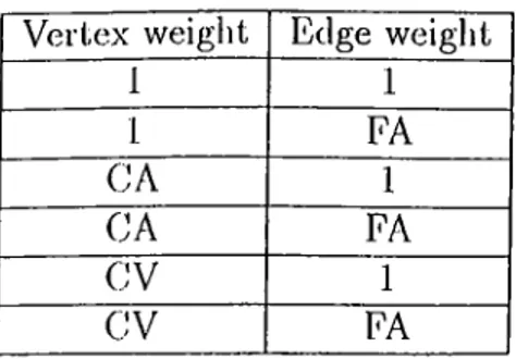
There are six possible weighting scheme combinations that can be used to determine the vertex and edge weights of the clusterization graph. These six [)ossibilities are shown in 'Table 3.1. 'The symbols CV, CA, FA denote the cell volume, c(ill area, and lace area., respectively. Unit cost scheme is represented by I.

For the edge weights it is more intuitive to u.se the FA scheme, since the total face area of a cluster better rei)i'esents that clusters interaction with the other clusters a.nd the screen. A cluster with large face areas has a higher chance to be hit by a ra.y. Using FA as edge weight produces spherical clusters which does not change their rendering loads by an important amount at different

Table 3.1. Possible weighting schemes for the clusterization graph.

Vertex weight Edge weight

1 1 1 FA CA 1 CA FA CV 1 CV FA

(41)

CHAPTER 3. IMACE-SPACE PA RA LLELIZATION 25

visualizations.

Also, we sot all vertex weights to 1 in the clusterization graph. This scheme pi’odnce.s clusters with equal cell size, and hence coinmnnication cost. The variation in the nniiiber of cells in clusters may be huge in CV and CA weighting schemes. Iixi)erimental results in Chapter 7 verifies our selection.

3.2.3 Additional Data Structures

Clustering the volume data requires the use of additional data structures. Each cluster is given a global identifier and a global ChsterMap array is crecited in every i)rocessor. This array is used to obtciin the cluster-processor mapping cind also to reach the data contciined within a cluster. Each element in this array niciintains pointer to the clusters local data, and a processor id showing tlie ])rocessor in which the cluster resides.

Processors keep only the data contained in their assigned clusters. Since each cluster stands as an entity that can be rendered independently, the data in the clusters are treated as local data. The Clusler data structure contains two arrays, namely local Nodes cind Cells arrays. Local indexing is utilized within these arrays.

Furthermore, the Cell data structure introduced in Cliapter 2 is modified such that now it includes information about the cluster identities, showing the neighl)or cluster for each face of a cell. Since a ray can leave a cluster from an tbficicc and enter into another cluster, it is necessary to know this new clusters identifier as a connectivity information. For internal faces the identifier of the cluster in which the face is located is assigned as the neighbor cluster identifier. These new and modified data structures are shown in Figure 3.3.

3.3 Load Balancing

Load balancing is one of the primary concerns in parallel applications. Without proper arrangement, an idle processor may drag the performance of the system

(42)

cu

A PTER S. IMAGE-SPACE PA RA LIEUZATION 26

(lowiiwaid. Iii ])arallel volunu; rciideriiig, (.lie readeiing load sliared among tlie processors should be balanced.

In structured grids, load babuicing is a relatively simple task. However, the lack of a simple indexing scheme in unstructured grids makes visualization cal culations on such grids very complex. Furthermore, unstructured grids contain data cells which are highly irregular in both size and shape. In a distributed comiMiting environment, irregularities in cell size and shajie make balanced load distribution very dilTicult.

3.3.1 Screen Subdivision

Since the aim in this work is image-space parallelization, the screen pixels and hence the load spread over them is tried to be equally shared among the pro cessors. Previous work on screen space subdivision methods includes the use of quad-trees, recursive bisection and jagged partitioning. All these methods a.ie common in that they try to divide the screen into rectangular pieces and distiibutc these sciiicn regions to processors. Ilowev(!r, since the division lines separating the regions are alwa.ys para.llel to the coordinate axis these subdi vision tcchiii(|U('s are not fh^xible enough and may not always produce |)crfect load balancing. Figure 3.4 displays these techniques on a screen with discre(,e load assignment.

The most flexible screen subdivision technique would be the one which makes the partition boundaries as flexible as possible, that is, sub-screen boundaries would be able to change to any shape. Unfortunately, this is not

struct Map { int procJd; Cluster *Clusters; } struct Cluster { Cell *Cells; Node *Nodes; int CellCount; int NodeCount; } struct Cell { int vertices[4]; int neighborCeIIs[4]; int neighboiFaces[4]; int neighborClusters[4]; }

(43)

CIIAPTFAt 3. IMAGE-SPACE PARALLEUZATION 27

a) Screen load distribution

■ ■ ■ ■ ■ ■ ■ ■ ■ ■ ■ ■ ■ ■ ■ ■ b) Quad-tree subdivision ■ ■ _■ ■ ■ . " ■ .... ■ ■ ■ ■ ■ ■ ■ ■ ■

c) Jagged subdivison d) Recursive subdivision

Figure 3.4. Screen .subdivision techniques.

practical for two reasons: First, excessive amount of processing is needed to determine and manipulate the non-regular sub-screen boundaries, and second, the data, structures to rei)resent the boundaries would be too complex a.nd might require too much storage.

In this work, the screen is subdivided by an n by n cartesian grid forming sub-regions, and this sub-regions are assigned to j)rocessors for rendering. hVoin now on, we will refer to these screen sub-regions as screen cells. VVe repres('iit the .set of screen cells by S. An individual screen cell in this set is represented by vi.

Since the projection area of the volume occupying the screen changes with respect to the visualization parameters, our approach requires the estimation of the grid granularity. In onr work, the number of i>ixels in screen cells is

(44)

CIIA PTER 3. IMAGE-SPACE PARA LLELIZATION 28

a) Coarse-grain grid b) Fine-grain grid

l''igLire 3.5. liffect of projection area on grid granularity.

determined adaptively. This is done by keeping the number of occupied (having a locid) screen cells constant at every visualization instance. This also prevents the variation in view dependent preprocessing time. Figure 3.5 shows the grid gi-anularities for two different projection area size. Note that, the number of occupied regions is nearly the same in both cases in the figure.

Adjusting the grid granularity such that each screen cell will contain just one pixel results in the most flexible screen cell boundaries mentioned above. However, increasing view dependent preprocessing overhead makes this ap proach iid’easible to use. On the contrary, it the number of screen celts is kept low, the solution space of the load l)alancing problem is reduced and satisfac tory load balance values cannot be obtained. We used an engineering formula, which is explained in Chapter A, to determine the appropriate granularity of the grid in an adaptive manner.

3.3.2 Work Load Calculation

In image-space parallelization, screen subdivision is not enough by itself to ob tain a good load bcilance. Also, the work load distributed over the pixels should be calculated correctly. The total work of rendering a cluster is approximated

A hypergraph-partitioning based remapping model for image-space parallel volume rendering

28S

A H Y P E R G R A P H -P A R T IT IO N IN G

BASED R E M A P P IN G M O D EL FOR

IM A G E -SP A C E PARALLEL

V O L U M E R E N D E R IN G

2000

•съа

A B S T R A C T

ÖZET

ACKNOWLEDGMENTS

Contents

List of Figures

List of Tables

List of Symbols and Abbreviations

c

s

y

z

Chapter 1

Introduction

1.1

Terminology and Classification

an A PTim i

i

f

1.2

Previous Work

[

]

[

]

]

[

]

[

] [

]

[

]

1.3

Proposed Work

с п л т т 1.

Chapter 2

Ray-Casting

2.1

Basic

R a y -

Casting Algorithm

2.2

Data Structures for Unstructured Grids

2.3

Koyamada’s Algorithm

an A PTica 2.

-

2.3.1

Intersection Test

2.3.2

Resampling

сил PTEll 2. RA Y-CASTING

2.4

Optimizations and Performance

Chapter 3

Image-Space Parallelization

3.1

OS versus IS Parallelization

3.2

Clusterization

3.2.1

Graph Partitioning

3.2.2

Weighting Scheme

3.2.3 Additional Data Structures

3.3

Load Balancing

cu

3.3.1

Screen Subdivision

3.3.2

Work Load Calculation