6
Cumulative Vehicle Routing Problems
(1)
İmdat Kara
1, Bahar Yetiş Kara
2and M. Kadri Yetiş
3 1Başkent University, Department of Industrial Engineering,
2Bilkent University, Department of Industrial Engineering,
3Havelsan A.Ş.7
thkm on Eskişehir Road,
Ankara,
Turkey
1. Introduction
The problems of finding optimal routes for vehicles from one or several depots to a set of locations/customers are known as Vehicle Routing Problems (VRPs) and have many practical applications, especially in transportation and distribution logistics. An extensive literature exists on these problems and their variations (e.g. Bodin(1990), Laporte(1992), Laporte & Osman(1995), Ball et al.(1995), Toth & Vigo (2002a)).
The Capacitated Vehicle Routing Problem (CVRP) is defined on a graph G = (V, A) where V={0,1,2, …, n} is the set of nodes (vertices), 0 is the depot (origin, home city), and the remaining nodes are customers. The set A = {(i, j): i, j ∈ V, i ≠ j} is an arc (or edge) set. Each
customer i ∈ V \ {0} is associated with a positive integer demand qi and each arc (i, j) is
associated a travel cost cij (which may be symmetric, asymmetric, deterministic, random,
etc.). There are m vehicles with identical capacity Q. The CVRP consists of determining a set of m vehicle routes satisfying the following conditions:
• Each route starts and ends at the depot,
• Each customer is visited by exactly one route,
• The total demand of each route does not exceed the vehicle capacity Q,
• The total “cost” of all routes is minimized.
The CVRP has been studied extensively in the literature (for recent publications, see e.g. Achutan et al. (1996), Toth & Vigo (2002b), Ralphs et al. (2003), Baldacci et al. (2004), Kara et al. (2004), Letchford & Salazar-Gonzalez (2006), Yaman (2006)). CVRP was first defined by Dantzig and Ramser in 1959. In that study, the authors used distance as a surrogate for the
cost function. Since then, the cost of traveling from node i to node j, i.e., cij, has usually been
taken as the distance between those nodes.
The real cost of a vehicle traveling between two nodes depends on many variables: the load of the vehicle, fuel consumption per mile (kilometer), fuel price, time spent or distance traveled up to a given node, depreciation of the tires and the vehicle, maintenance, driver wages, time spent in visiting all customers, total distance traveled, etc. (Baldacci et al. (2004), Toth & Vigo (2002a), Desrochers et al. (1990)). Most of the attributes are actually distance or
1A preliminary version of this paper has appeared in the proceedings of the First
International Conference on Combinatorial Optimization and Applications, COCOCA 2007, Xi’an, China, (Kara et al., 2007).
time based and can be approximated by the distance. However, some variables cannot be represented by the distance between nodes. Examples of such variables are vehicle load, fuel consumption per mile (kilometer), fuel price, time spent up to a given node. Most of these types of variables may be represented as a function of the flow on the corresponding arc (load or weight of the vehicle, number of items on the vehicle, the order in the tour of starting and/or ending node of the arc and etc.). Thus, for some cases, in addition to the distance traveled, we need to include flow on the related arc as another indicator of the cost. In this study, we propose a cost function which is defined as a product of the distance traveled and the flow on that arc. To the best of our knowledge, the vehicle routing literature has not previously included such a definition of cost, which is the main motivation of this research.
In the VRP, vehicles collect and/or deliver the items and/or goods from/to each customer on the route. Thus, the flows on the arcs change throughout the tour. They show an increasing step function in the case of collection and a decreasing step function in the case of delivery. So, flows cumulate or diminish along the tour. For this reason, we call a CVRP with flow based cost function as the Cumulative Vehicle Routing Problem, abbreviated as CumVRP.
The main contribution of this paper may be summarized as:
• Define a new cost function for vehicle routing problems as a multiple of length of the
arc traveled and the flow on this arc. Name this problem as Cumulative Vehicle Routing Problem (CumVRP).
• Present polynomial size integer programming formulations for CumVRP for collection
and delivery cases.
• Show the relationship between the proposed CumVRP with the m-Traveling
Repairman and related problems .
• Illustrate the use of CumVRP in the real life situations such as energy minimizing VRP
and school-bus routing problems.
We provide problem identification and integer programming formulations of the CumVRP for both collection and delivery cases in Section 2. In Section 3, we show that the proposed problem is a generalization of the m-Traveling Repairmen Problem, and so is relevant to minimum latency and its variations mentioned in the literature. Two additional applications of the flow-based cost function, namely the Energy-Minimizing VRP and the Average-Distance Minimizing School Bus-Routing Problem, are also illustrated in the same section. The proposed models are tested and illustrated by real life data from Turkey and the results are given in Section 4. Concluding remarks are in Section 5.
2. Formulations of the CumVRP
In this section, details of the Cumulative Vehicle Routing Problem are outlined and then integer linear programming formulations are presented.
2.1 Problem identification
Consider a vehicle routing problem defined over a network G = (V, A) where V={0,1,2, …, n} is the node set, 0 is the depot and A = {(i, j): i, j ∈ V, i ≠ j} is the set of arcs, and, components are given as:
Parameters:
dij is the distance from node i to node j.
qi is the nonnegative weight (e.g. demand or supply) of node i.
Q0 is the initial value of flow from the origin to the first node of the tour in the case of
collection, or the final value of flow from the last node of the tour to the origin in the case of the delivery, ( e.g. tare of the truck in the case of carrying goods).
M represents the flow capacity of the arcs of the network (maximal value of the flow on
any arc of the network, for example, capacity plus tare of the trucks in the case of carrying goods).
Decision Variables:
xij = 1 if the arc (i, j) is on the tour of a vehicle, and zero otherwise;
yij is the flow on the arc (i, j) if the vehicle (traveler) goes from i to j, and zero otherwise.
Cost:
The cost of traversing an arc (i , j), cij, is defined as the product of the distance of the arc (i , j)
and flow on this arc.
With those given above, we define Cumulative Vehicle Routing Problem (CumVRP) as:
• Each node (customer) is served exactly by one vehicle.
• Each route starts and ends at the depot.
• For each tour, the flow on the arcs cumulate as much as preceding node’s supply in the
case of collection or diminish as much as preceding node’s demand in the case of delivery.
• The flow on any arc of each tour doesn’t exceed the flow capacity of the arcs.
• The objective is to find a set of m vehicle routes of minimum total cost where the cost is
defined as the product of the distance of the arc (i , j) and flow on this arc.
Definition of the yij’s is the core of this approach. The flow on the first arc of any tour must
take a predetermined value and then must always increase (or decrease) by qi units just after
node i. In the case of collection, the flow variable shows an increasing step function; for delivery, it shows a decreasing step function. Therefore a model constructed for collection case may not be suitable for the delivery case. The following observation states the relationship between them.
Observation 1: When the distance matrix is symmetric, the optimal route of the delivery (collection) case equals the optimal route of the collection (delivery) case traversed in the reverse order.
Proof: Consider a route which consist of k nodes: n0-n1-n2-…-nk-n0, where n0 is the depot.
For the collection case, the cost of this tour is:
1 0 01 0 , 1 0 0 1 1 1 j k k i j j i k j i i Q d − Q q d + Q q d = = = ⎛ ⎞ ⎛ ⎞ +
∑
⎝⎜ +∑
⎠⎟ +⎝⎜ +∑
⎠⎟ (1)For the delivery case, the cost of the reverse route n0-nk-nk-1-…-n1-n0 is:
1 0 0 0 1, 0 10 1 1 1 j k k i k i j j i j i Q q d − Q q d+ Q d = = = ⎛ ⎞ ⎛ + ⎞ + + + ⎜ ⎟ ⎜ ⎟ ⎝
∑
⎠∑
⎝∑
⎠ (2)Observe that (1) and (2) are the same for symmetric D=[dij] matrices.
2.2 Mathematical models
For the symmetric-distance case, one does not need to differentiate between collection and delivery since the solution of one will determine the solution of the other. For the case of an
asymmetric distance matrix, due to the structure of the problem, we present decision
models for collection and delivery cases, separately. The model for the collection case is:
F1: 0 0 n n ij ij i j Min d y = =
∑∑
(3) s.t. 0 1 n i i x m = =∑
(4) 0 1 n i i x m = =∑
(5) 0 1 n ij i x = =∑
(6) 0 1 n ij j x = =∑
(7) 0 0 n n ij ji i j j j i j i y y q = = ≠ ≠ − =∑
∑
i = 1, 2, …, n (8) y0i =Q0 x0i i = 1, 2, …, n (9) ( ) ij j ij y ≤ M q x− (i , j) ∈ A (10) 0 ( ) ij i ij y ≥ Q +q x ( , )∀ i j ∈A (11) 0 1 ij x = or , (i , j) ∈ A (12) Where q0 = 0.The objective function given in (3) gives the proposed cost function. Constraints (4) and (5) ensure that m vehicles are used. Taking “≤” instead of “ = “ in these relation is also possible when one imposes to use at most m vehicle. Constraints (6) and (7) are the degree constraints for each node, together with (4) and (5), they are called assignment constraints of the formulation. Constraint (8) is the classical conservation of flow equation balancing inflow and outflow of each node, they guarantee that, flow variables of each tour perform an increasing step function. Those constraints also prohibit any illegal subtour. Constraint (9) initialize the flow on the first arc of each route, cost structure of the problem necessitates
such an initialization. Constraints (10) take care of the capacity restrictions and forces yij to
zero when the arc (i,j) is not on any route, and constraint (11) produce lower bounds for the flow on any arc. Integrality constraints are given in (12). We do not need nonneqativity
constraints for yij’s since we have constraints given in (11).
Let us call constraints (9), (10) and (11) as the bounding constraints of the formulation . Validity of these bounding constraints is shown in proposition 1 below.
Proposition 1: In the case of collection, the constraints given in (9), (10) and (11) are valid for CumVRP.
Proof: As it is explained before, we need initialization value of yij’s for each tour that
constraints (9) do it, otherwise yij’s may not be actual flow on the arcs. Constraints (11) is
valid since going from i to j the flow must be at least the initial value plus the weight of the
node i (unless node i is the depot, in which case q0 = 0). Similarly, since the vehicle is
destined for node j, it will also collect the weight at node j (unless j is the depot). In that case, the flow on the arc upon arriving at node j should be enough to take the weight of node j,
i.e.,
y
ij+
q
jx
ij≤
Mx
ij, which produce constraints (10).□Similar constraints for classical CVRP may be seen in (Gouveia (1995), Baldacci et al.(2004), Letchford & Salazar-Gonzalez (2006), Yaman (2006)).
Due to Observation 1, the delivery problem for the symmetric case need not be discussed. For the asymmetric case, the delivery problem will be modeled by replacing constraints (8) ,(9), (10) and (11) with the following given below.
0 0 n n ji ij i j j j i j i y y q = = ≠ ≠ − =
∑
∑
for i=1,2,….,n (13) yi0 =Q0 xi0 for i=1,2,….,n (14) ( ) ij i ij y ≤ M q x− ( , )∀i j ∈A (15) 0 ( ) ij j ij y ≥ Q +q x ( , )∀i j ∈A (16) Thus the model for the delivery case is:F2: 0 0 n n ij ij i j Min d y = =
∑∑
s.t. (4)-(7),(12) - (16). where q0=0.Both of the proposed models have n2+n binary and n2+n continuous variables, and
2n2+6n+2 constraints, i.e., proposed formulations contain O(n2) binary variables and O(n2)
constraints.
3. Applications of the CumVRP
In this section, we show that the special case of the CumVRP turns out some routing problems, namely, Minimum Latency Problem, m-Traveling Repairman Problem, Energy Minimizing Vehicle Routing Problem and School-bus Routing Problem.
3.1 Relevance to minimum latency and related problems
The Time-Dependent Traveling Salesman Problem (TDTSP) is a generalization of the standard Traveling Salesman Problem in which the cost of traveling from one node to another depends not only on the two locations, but also on their positions in the tour (Picard &
Queyranne (1978), Lucena (1990), Gouviea & VoB (1995)). When the objective of the TDTSP is to minimize the sum of distances traveled from the depot to all nodes, the problem is known as the Traveling Salesman Problem with Cumulative Cost or the Cumulative Traveling
Salesman Problem (CTSP), as defined by Bianco et al.(1993). The CTSP is exemplified by pizza
delivery since the time it takes the pizza to reach the customer is determined by the total travel time from the depot.
Latency of a node is defined as the total distance traveled up to that node. The Minimum
Latency Problem is to find a tour starting at a depot and visiting all nodes in such a way that
the total latency is minimized (Archer et al. (2003), Blum et al. (1994)). This problem is also known as the Delivery Man Problem (Fischetti et al. (1993)) or the Traveling Repairman Problem (Jothi & Raghavachari (2007)).
We conclude therefore that, the Cumulative Traveling Salesman Problem, the Minimum Latency Problem and the Traveling Repairman Problem are all same with respect to the structure of their objective functions.
The Multiple Traveling Repairman Problem (mTRP) is a generalization of the Minimum Latency Problem (hence repairman) and finds m tours, each starting at the depot and covering all the nodes while minimizing total latency (Jothi & Raghavachari 2007).
We now investigate the relations between the CumVRP and the mTRP.
Lemma 1: mTRP is a special case of the delivery formulation of CumVRP, where Q0 =1 and
qi =1 for all i=1, 2, …, n and M = n-m+2.
Proof: Consider delivery formulation of CumVRP. Define yij as the number of remaining
arcs on the tour from the node i to the origin if traveler goes from i to j, zero otherwise. Letn
Q0 =1, and qi =1 for all i=1,2,…,n. For each tour, the corresponding yij’s shows a descending
ordered integer sequences ending with 1. For such a case, consider a route composed of k
intermediate nodes as n0-n1-n2-…-nk-n0, where n0 is the depot. Let dij denote the distance
from ni to nj of this route and yij are the corresponding flow variables. Since there are (k+1)
nodes in this tour, in order to end with value 1, the starting value of yij must be (k+1). So the
part of the objective function of the CumVRP model corresponding to the this route is,
(k+1)d01+kd12+(k-1)d23+……+dk0, (17)
which can be rewritten as,
d01 + (d01 +d12 )+ (d01 +d12 +d23)+…..+ (d01 +d12 +d23+…+dk0). (18)
As can be seen, expression (18) is the sum of the latencies of the nodes on this tour. Thus, the CumVRP formulation for this delivery problem involves finding m tours, each starting at the depot, such that the total latency up to each node is minimized; this is nothing but the mTRP problem. Hence, mTRP is a special case of the delivery formulation of the CumVRP. For this special case, m-1 traveler (repairman) may visit only one node and turn back to the depot. So maximal intermediate nodes on a tour will be n-(m-1) = n-m+1, which implies that, the value of the M in the formulation, i.e., the maximal number of arc on a tour, must
be taken as n-m+1. Using Lemma 1, letting qi =1 for all i, Q0 =1and M=n-m+1 in formulation
F2, we produce a formulation for mTRP and so we propose an integer programming
F3: 0 0 n n ij ij i j Min d y = =
∑∑
(3) s.t. (4)-(7) ,(12) and 0 0 1 n n ji ij j j j i j i y y = = ≠ ≠ − =∑
∑
for i=1,2,….,n (19) yi0 = xi0 for i=1,2,….,n (20) ( ) ij ij y ≤ n m x− i 0, ( , )≠ ∀i j ∈A (21) 2 ij ij y ≥ x j 0, ( , )≠ ∀i j ∈A (22) In this formulation, constraints (19)-(22) play same role as the corresponding constraints doin F2In the formulation F3, if we take m=1, i.e., one traveler, we get an integer linear programming formulation for Minimum Latency (Traveling Repairman and Cumulative Traveling Salesman) Problem. Consequently, CumVRP produces a unified formulation for these special routing problems also.
It has been shown in the literature that the CTSP and related problems including the mTRP are NP-hard (Tsitsiklis (1992), Archer et al (2003)). Due to the Lemma 1, we conclude that CumCVRP is NP-hard.
For some cases of the mTRP (e.g. delivering pizza), the distance (or traveling time) of the last arc on the tour may not be considered in the objective function.
3.2 Energy minimizing vehicle routing problem [Kara et al., (2007)]
For vehicle routing problems where vehicles carry goods from an origin (center, factory and/or warehouse) to the customer, or from the customer to the origin, the traveling cost between two nodes can be written as,
Cost = f(load, distance traveled, others)
where f(.) is any function. We derive a cost function that mainly focuses on the total energy consumption of the vehicles. Recall from mechanics that,
Work = force * distance
In the VRP, the movement of the vehicles can be considered as an impending motion where the force causing the movement is equal to the friction force (see for example Walker (2000)). Remember also that,
Friction force = Coefficient of friction * weight. Thus, we have
Work = Friction force * distance. Work = Coefficient of friction * weight * distance
The coefficient of friction can be considered as constant on roads of the same type. Then, the work done by a vehicle over a link (i, j) will be:
Work = weight of the vehicle (over link (i, j)) * distance (of link (i, j)).
Since work is energy, minimizing the total work done is equivalent to minimizing the total energy used (at least in terms of fuel consumption). Obviously, the weight of the vehicle equals the weight of the empty vehicle (tare) plus the load of the vehicle. Thus, if one wants to minimize the work done by each vehicle, or to minimize the energy used, one needs to use the cost as,
Cost of (i, j)= [Load of the vehicle over (i , j)+Tare] * distance of (i, j), (23)
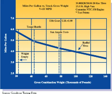
There seems to be no such definition and objective cost function in the vehicle routing literature. However, there are references on the Internet (such as the Goodyear website) indicating that fuel consumption changes with vehicle load. The figure-1 below depicts the miles per gallon as a function of the total load.
Clearly, miles per gallon decrease with increased vehicle weight. Thus for a VRP in which goods are carried and fuel prices are relatively more important than the drivers’ wages, considering the load of the vehicle as well as the distances will produce a more realistic cost of traveling from one customer to another. This analysis shows that for such VRP’s we may define a more realistic cost of traveling from one customer to another by considering the load of the vehicle as well as the distances. We refer the VRP in which cost is defined as in expression (23) as the Energy Minimizing Vehicle Routing Problem, this being a special case of the CumVRP as shown below.
Figure 1. Miles per Gallon versus vehicle weight (http://www.goodyear.com/truck/pdf/ commercialtiresystems/FuelEcon.pdf).
In CumVRP, let us define yij as the total weight of the truck while traversing the arc (i, j); qi ‘s are supply (collection) or demand (delivery) of ith customer; Q0 is the tare of the truck, Q is the capacity of each truck and M = Qo+Q. With these definitions, substituting Qo+Q instead of M in F1 and F2 , we get integer programming formulations of the collection and delivery cases of the Energy Minimizing Vehicle Routing Problem, respectively.
3.3 School-bus routing problem
School-bus routing is a primary application of the VRP; the question is how to transport students to and from school in an optimal way (Bodin (1990); Corberan et al. (2002)). The children are assigned to bus stops and a sequence of individual stops will form a bus route. In the morning, the buses pick up the students from bus stops and take them to the school; the procedure is reversed in the afternoon (Bodin (1990); Swersey & Ballard (1984)). Each school bus routing problem has different objectives and/or constraints. Bus capacity, the maximum number of stops per bus, the maximum length (or duration) of each tour and student riding time are the most frequently encountered additional requirements. There are different objectives, such as: minimizing transportation cost, minimizing transportation time, minimizing the time that a student spends on the bus, minimizing the number of buses required, minimizing fleet travel time, and balancing bus loads and route lengths (Corberan et al.(2002); Li & Fu (2002)).
For a school-bus routing problem, suppose the decision maker wants to evaluate alternative routes with respect to average distance traveled (or average time spent) per student. We could find no such objective in the literature. Let us define this problem as the
Average-Distance Minimizing School-Bus Routing Problem. The CumVRP formulation can be used to
solve such a school-bus routing problem.
Because of the asymmetric nature of road traffic at different times of a day, the collection and delivery cases in school-bus routing problems must be handled separately. Let us define
V= {0, 1, 2… n} as a set of nodes (vertices), where {0} is the school and the remaining nodes
are bus stops. Let the set A, the distances between two nodes dij and the binary variables xij
be defined as in Section 2.1. Define yij as the number of students in the bus while it is
traveling on the arc (i, j) if the bus passes from bus stop i to bus stop j, zero otherwise. We assume that the buses start their tour in the morning from the parking place and end at the school. In the afternoon, the tours begin from the school and ends at the parking place. For simplicity, we assume that the parking place is at the school. In computing the average distance traveled per student, the distance (or time) from the parking place to the first pick-up point in the collection case, and the distance from the last stop to the parking place in the
delivery case, must not be considered; therefore Q0 is equal to zero in both cases.
Consider a school bus problem where Cap denotes the capacity of the bus and qi denotes the
number of students boarding or disembarking at stop i. Then any average-distance
minimizing school-bus routing problem is equivalent to CumVRP where Q0=0 and M =
Cap. So then with these parameters, F1 will be a formulation for morning tours (collection)
and F2 will be a formulation for afternoon tours (delivery).
If there are other restrictions besides bus capacity, these constraints can easily be incorporated into the model. If the objective is defined as minimizing the average time spent per student, it is only necessary to measure the time needed to travel between the nodes of
4. Illustrative examples and computational analsis
In this section, we conduct some numerical examples of CumVRP formulation focusing on the collection case of the Energy Minimizing VRP.
We solve the instances via CPLEX 8.1. on an Intel Pentium III 1400 MHz computer. We want to test the effect of the new objective function on the optimal routes (i.e. distance-based routes versus energy-based routes).
The Energy Minimizing model of CumVRP is tested for realistic instances by using the data from the Turkish highway map. In this demonstration, customers correspond to the cities and we assume that there is a main collection center at Ankara, the capital of Turkey. A truck starting at this center collects the goods from each city towards Ankara. In Turkey there are 81 cities. We used the most industrialized 31 cities in our analysis. We also generated a smaller set with 24 cities to test the performance of the model with respect to increase in the number of nodes. We did not include Istanbul in our computational analysis since the volume generated there is large enough for a dedicated trip to Istanbul.
Our model has 5 types of parameters: travel distances between each city pair, the demand of each city, the number of trucks (vehicle), tare and capacity of a truck. For the travel distances, we used the data proposed by Tan & Kara (2007)) which is available at (www.bilkent.edu.tr\~bkara/hubloc.htm). For the demand of each city we assumed that
each individual generates 10-5 kg of reusable materials and so scaled the population of each
city with that tare. Truck capacity is taken as 100 units whereas tare has been taken as 15% of the capacity.
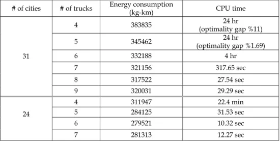
We varied the number of trucks by starting from the minimum possible number, which is 3 for both cases, up to the largest meaningful number, which is 8 for 31 cities and 6 for 24 cities. As can be seen in Table 1, increasing the number of trucks to values more than those numbers, results in the cost increasing since the model forces to use that many trucks by assigning dedicated trips to certain cities and so the cost increases even though we increase the number of trucks.
In Table 1, we present the objective function values, and the CPU hours provided by CPLEX. We terminate when the CPU time reaches 24 hours.
# of cities # of trucks Energy consumption (kg-km) CPU time
4 383835 (optimality gap %11) 24 hr 5 345462 (optimality gap %1.69) 24 hr 6 332188 4 hr 7 321156 317.65 sec 8 317522 27.54 sec 31 9 320031 29.29 sec 4 311947 22.4 min 5 284125 31.53 sec 6 279521 10.32 sec 24 7 281313 12.27 sec
For 31 cities, the CPU time increases as the number of trucks decreases. For 4 and 5 trucks, we terminated after 24 hours and reported the optimality gap. However, when the number of trucks is 7 or more, the optimum solutions are obtained within seconds. When we decrease the number of cities to 24, the CPU time decreases drastically. Even the 4 truck case is solved within minutes.
Next, we wanted to observe the effect of the objective function on the optimal routes. For each (# of city, #of truck) combination, we generated two instances: one with the energy minimizing objective, and the other with the distance minimizing objective (the one customarily used in the literature). For each instance, we report the energy used and the distance of the corresponding solution in Table 2. We also calculate the percent deviation of each value from the best possible (e.g. [Energy consumption of the distance minimizing routes] / [Energy consumption of the energy minimizing routes])
Minimizing Energy Minimizing Distance
# of city # of truck Energy consumptio n (kg*km) Distance traveled (km) Percent from the best distance value Energy consumptio n (kg*km) Distance traveled (km) Percent from the best energy value 4 383835 9056 1,13 450907 8012 1,17 5 345462 9517 1,15 424602 8304 1,23 6 332188 10511 1,22 434119 8649 1,30 7 321156 11379 1,25 421770 9115 1,31 31 8 317522 11914 1,23 437255 9683 1,38 4 311947 8423 1,16 401120 7284 1,29 5 284136 8857 1,15 374798 7677 1,32 24 6 279521 9656 1,17 343374 8269 1,23 Table 2. The results under both scenarios
As can be seen in Table 2, the energy consumption of the routes which minimizes the total distance traveled can be up to 38% (31 cities, 8 trucks case) over the best possible energy consumption. Meanwhile, minimizing the energy consumption can increase the total distance traveled as much as %25.
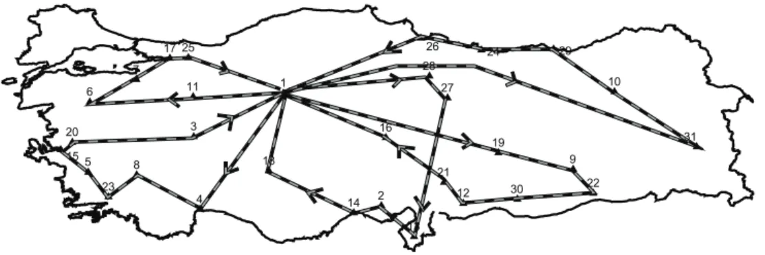
Also observe from Table 2 that, when the objective is total distance traveled, the smallest possible and largest meaningful numbers of trucks are equal (4 for both 24 and 31 cities). When we increase the number of trucks to 5 or more, the total distance traveled increases as the solution includes dedicated trips to certain cities (the ones closer to main depot Ankara). However, when the objective also includes the weights of the trucks, the cost could be decreased by the addition of the new trucks. The figures 2 and 3 demonstrate the solutions for 31 cities and 5 trucks.
Observe from the figures 2 and 3 that the routes of the two cases are very different from each other. The eastern cities generate smaller volume and so 10 of them can be served by one truck (Figure 3). However, when we include the weights in the objective, the two routes are split into three routes.
Even though we proposed a model with O(n2) binary variables and O(n2) constraints for the
therefore necessary to develop efficient solution procedures for each special cases of the CumVRP, like heuristics proposed for CVRP (Gendreau, et al.,(1994); Toth & Vigo(2003)). However, these modifications are beyond the scope of this paper.
$ $ $ $ $ $ $ $ $ $ $ $ $ $ $ $ $ $ $ $ $ $ $ $ $ $ $ $ $ $ $ 7 6 1 3 5 8 9 4 2 26 24 29 17 25 28 10 11 27 20 15 31 16 19 18 21 23 12 30 22 14 13
Figure 2. The energy minimizing routes with 5 trucks
$ $ $ $ $ $ $ $ $ $ $ $ $ $ $ $ $ $ $ $ $ $ $ $ $ $ $ $ $ $ $ 7 6 1 3 5 8 9 4 2 26 24 29 17 25 28 10 11 27 20 15 31 16 19 18 21 23 12 30 22 14 13
Figure 3. The distance minimizing routes for 5 trucks
5. Conclusion
This paper proposes a new objective function and corresponding formulations for the vehicle routing problem. The new cost function defined as the product of the distance of the arc and the flow on that arc. We call a vehicle routing problem with this new objective function as the Cumulative Vehicle Routing Problem (CumVRP). Integer programming
formulations with O(n2) binary variables and O(n2) constraints are developed for both
collection and delivery cases. We show that the CumVRP is a generalization of the m-Traveling Repairman and related problems in the literature; as an additional finding, we
propose an integer programming formulation with O(n2) constraints and decision variables
for the m-Traveling Repairman Problem. We discuss two additional applications of the CumVRP: the Energy-Minimizing VRP and the Average Distance-Minimizing School-Bus Routing Problem.
The collection case of the proposed models for Energy Minimizing case of the CumVRP are tested and demonstrated by using CPLEX 8.1 on some problems from Turkey’s 31 and 24
city distance data. We conclude that, increasing the number of vehicles up to a threshold value causes a decrease in the total energy used. We also observed that, CPU time increases as the number of the vehicles decreases. As expected, the number of the customer, i.e., the number of the nodes of the related network, effects CPU times directly. Distance minimizing and energy minimizing solutions of the same problem indicate that, energy minimizing routes travel over longer distances than distance minimizing solutions and optimal routes of the distance minimizing case consume more energy than the other.
Developing good heuristics for each special case of CumVRP and to conduct a computational analysis for comparing integer programming formulations of m-TRP problems are possible future research extensions.
6. Acknowledgment
The authors would like to express their sincere thanks to Gilbert Laporte for his valuable comments and suggestions on an earlier version of this manuscript.
7. References
N.R. Achutan, L. Caccetta, and S.P. Hill. (1996). A new subtour elimination constraint for the vehicle routing problem, European Journal of Operational Research 91 573-586.
A. Archer, A. Levin and D. P. Williamson.( 2003). Faster approximation algorithms for the minimum latency problem, in Proceedings of 14th Symposium of Discrete
Algorithms(SODA), 88-96
R. Baldacci, E. Hadjiconstantinou and A. Mingozzi. (2004) .An exact algorithm for the capacitated vehicle routing problem based on a two-commodity network flow formulation, Operations Research 52 723-738.
L. Bianco, A. Mingozzi and S. Ricciardelli. (1993). The traveling salesman problem with cumulative costs, Networks, 23, 81-91.
A. Blum, P. Chalasani, D. Coppersmith, B. Pulleyblank, P. Raghavan and M. Sudan. (1994). The minimum latency problem in STOC, 163-171.
L.D. Bodin. (1990). Twenty years of routing and scheduling, Operations Research 38(4), 571-579. A. Corberan, E. Fernandez, M. Laguna and R. Marti. (2002). Heuristic solutions to the
problem of routing school buses with multiple objectives, Journal of the Operational
Research Society 53, 427-435.
G.B. Dantzig and J.H. Ramser. (1959). The truck dispatching problem, Management Science, 6, 80-91.
M. Desrochers, J. K. Lenstra and M. W. P. Savelsbergh. (1990). A classification scheme for vehicle routing and scheduling problems, European Journal of Operational Research, 46, 322-332.
M. Fischetti, G. Laporte and S. Martello. (1993). The delivery man problem and cumulative matroids, Operations Research, 41(6), 1055-1064.,
M. Gendreau, A. Hertz, and G. Laporte. (1994). A tabu search heuristic for the vehicle routing problem, Management Science, 40, 1276-1290.
L.Gouveia. (1995). A result on projection for the vehicle routing problem, European Journal of
Operational Research, 856, 10-624.
L.Gouveia and S. VoB. (1995). A classification of formulations for the (time-dependent) traveling salesman problem, European Journal of Operational Research, 83, 69-82.
R. Jothi and B.Raghavachari. (2007). Approximating the k-traveling repairman problem with repair times, Journal of Discrete Algorithms, 5, 293-303.
İ. Kara, G. Laporte and T. Bektaş. (2004). A note on the lifted Miller-Tucker-Zemlin subtour elimination constraints for the capacitated vehicle routing problem, European
Journal of Operational Research, 158, 793-795.
I. Kara, B.Y.Kara, and K.Yetis, (2007). Energy minimizing vehicle routing problem. In A.Dress, Y.Xu, and B. Zhu (Eds), Combinatorial Optimization and Applications, LNCS Vol. 4616, pp. 62-71.
G. Laporte. (1992). The vehicle routing problem: An overview of exact and approximate algorithms, European Journal of Operational Research , 59 345-358.
G. Laporte and I.H. Osman. (1995) Routing problems: A bibliography, Annals of Operations
Research, 61, 227-262.
A. N. Letchford and J-J Salazar-Gonzalez. (2006). Projection results for vehicle routing,
Mathematical Programming, Ser. B 105, 251-274.
L. Li and Z. Fu. The school bus routing problem: a case study, Journal of the Operational Research Society 53(2002) 552-558.
A. Lucena. (1990). Time-dependent traveling salesman problem-The deliveryman case,
Networks, 20, 753-763.
J.C. Picard and M. Queyranne. (1978). The time-dependent traveling salesman problem and its application to the tardiness problem in one-machine scheduling, Operations
Research, 26(1), 86-110.
T.K. Ralphs, L. Kopman, W.R. Pulleyblank and L. E. Trotter. (2003). On the capacitated vehicle routing problem, Mathematical Programming Series B, 94 343-359.
A.J. Swersey and W. Ballard. (1984). Scheduling school buses, Management Science, 30(7), 844-853.
P. Tan and B.Y. Kara (2007). “A Hub Covering Model for Cargo Delivery Systems”,
Networks, 49(1), 28-39.
P. Toth and D. Vigo. (2002a). An overview of vehicle routing problems. In: P. Toth and D. Vigo, (editors). The Vehicle Routing Problem. SIAM Monographs on Discrete
Mathematics and Applications. SIAM, 1-26.
P. Toth and D. Vigo. (2002b) Models, relaxations and exact approaches for the capacitated vehicle routing problem, Discrete Applied Mathematics 123, 487-512.
P. Toth and D. Vigo. (2003). The Granular Tabu Search and its application to the vehicle routing problem, INFORMS Journal on Computing,15(4), 333-346.
J.N. Tsitsiklis. (1992) Special cases of traveling salesman and repairman problems with time windows, Networks, 22, 263-282.
K. M. Walker. (2000). Applied Mechanics for Engineering Technology (sixth edition), Prentice Hall.
H. Yaman. (2006). Formulations and valid inequalities for the heterogeneous vehicle routing problem, Mathematical Programming, Ser. A ,106 365-390.