Multilead ECG data compression by multirate signal processing and transform domain coding techniques

ШёшшЁШ вшмш шѳ&ішё іш ш т ш ш

nmêrtmL· -Щ'ЛШѣшш of

2120ТѢС>^йСЗ £^^GIïí£ESlï.:G

J.ME; ІШ : ííW STOTS OF Ш0> SCsSàiCSS

О? ш і-тѵ? ш ^г/£ш ту 2ií я ш й и і OF τ ϊ^

шоиівтшш

? 'Ж Tií£ 0 £ Э 2£ £ OF І Ш 5 ^ Of SGSBNOE lAi β ’УШ'. ( - · · > / Ä P /

MULTILEAD EGG DATA COMPRESSION BY

MULTIRATE SIGNAL PROCESSING AND

TRANSFORM DOMAIN CODING TECHNIQUES

A T H E S IS S U B M IT T E D TO T H E D E P A R T M E N T O F E L E C T R IC A L A N D E L E C T R O N IC S E N G IN E E R IN G A N D T H E IN S T IT U T E O F E N G IN E E R IN G A N D SC IE N C E S O F B IL K E N T U N IV E R S IT Y IN P A R T IA L F U L F IL L M E N T O F T H E R E Q U IR E M E N T S F O R T H E D E G R E E O F M A S T E R O F S C IE N C E

By

M. Cengiz Aydın

July 1991

■

mı

mı

(ç) Copyright July, 1991

by

I certify that I have read this thesis and that in my opinion it is fully adequate, in scope and in quality, as a thesis for the degree of Master of Science.

x A · - ? .

Assoc. Prof. Dr. A. Enis Çetin(Principal Advisor)

I certify that I have read this thesis and that in my opinion it is fully adequate, in scope and in quality, as a thesis for the degree of Master of Science.

Prof//Dr. Hayrettin Köymen

I certify that I have read this thesis and that in my opinion it is fully adequate, in scope and in quality, as a thesis for the degree of Master of Science.

Approved for the Institute of Engineering and Sciences:

/ i 'f

-Jiaray Prof. Dr. Mehmet Haray

ABSTRACT

MULTILEAD EGG DATA COMPRESSION BY MULTIRATE

SIGNAL PROCESSING AND TRANSFORM DOMAIN

CODING TECHNIQUES

M. Cengiz Aydın

M.S. in Electrical and Electronics Engineering

Supervisor: Assoc. Prof. Dr. A. Enis Çetin

JuR 1991

This thesis presents two data compression methods for digital electrocardio­ gram (EGG) signals. The first method is proposed for the compression of single lead EGG data. Various coding technicgies such as Sub-Band Transform and Variable Length Godings are used to realize that purpose. Data size reduction which is a problem in EGG databases is chosen as an aiDplication and successful results are cichieved during simulations. The second algorithm is proposed for the multilead EGG data compression. A linear transform is applied to samples of the eight standard EGG lead signals. The resulting transform domain sig­ nals are compressed using \'arious coding methods, including multi-rate signal processing and transform domain techniques. Higher compression ratios are achieved compared to the single channel compression techniques.

Keywords: EGG Data Gompression, Sub-Band Goding, Transform Goding.

ÇOK UÇLU EKG VERİLERİNİN ÇOK ÖRNEKLEME

FREKANSLI İŞARET İŞLEME VE DÖNÜŞÜM DÜZLEMİ

KODLAMA TEKNİKLERİ KULLANILARAK

SIKIŞTIRILMASI

M. Cengiz Aydın

Elektrik ve Elektronik Mülıendisliği Bölümü Yüksek Lisans

Tez Yöneticisi: Doç. Dr. A. Enis Çetin

Temmuz 1991

Bu tezde sayısal elektrokardiogram (EKG) i-şaretlerinin sıkıştırılması için iki ayrı yöntem sunulmaktadır. İlk yöntem tek uçlu EKG verilerinin sıkıştırıl­ masını amaçlar. Bu amacı gerçekleştirmek için Alt-Bant-Kodlaması, Dönüşüm Düzleminde Kodlama ve Değişken Uzunluklu Kodlama gibi çeşitli 3'öntemler kullanılmıştır. EKG veri tabanlarının problemi olan veri hacmi azaltılması uy­ gulama olarak seçilmiş ve benzetim sırasında başarılı sonuçlar elde edilmiştir. İkinci yöntem çok uçlu EKG verilerinin sıkıştırılması için önerilmektedir. Se­ kiz EKG kanalına ait veriler lineer bir dönüşümden geçirilirler. Bu dönüşüm sonucu oluşan işaretler Çok Örnekleme Frekanslı İşaret İşleme ve Dönüşüm Düzleminde Kodlama teknikleri kullanılarak sıkıştırılırlar. Böylece, tek kanallı sıkıştırma yöntemlerine göre daha yüksek sıkıştırma oranlarına ulaşılmaktadır.

Anahtar Sözcükler: EKG verilerinin sıkıştırılması, Alt-Bant-Kodlaması, Dönüşüm Düzleminde Kodlama.

ACKNOWLEDGMENT

I would like to thank my supervisor Assoc. Prof. Dr. A. E. Çetin for his in­ valuable guidance during the preperation of this thesis. I would also appreciate Prof. Dr. Hayrettin Köymen and Assoc. Prof. Dr. Mehmet Ali Tan for their helpful suggestions.

1 Introduction 1

1.1 ECG Waveform and Standard Lead S y s te m s ... 2 1.2 ECG Compression Techniques: A R eview ... 5 1.2.1 Definitions of Compression Ratio and Reconstruction Error 6 1.2.2 Direct ECG Data Compression Techniciues... 7 1.2.3 Transform Domain Compression T ech n iq u es... 11

2 Single Lead ECG D ata Com pression 13

2.1 Description of the p ro ce d u re ... 13 2.2 Simulation re s u lts ... 17

3 M ultichannel ECG D ata C om pression 20

3.1 Description of the Procedure; 20

3.1.1 The P rep ro cesso r... 21

3.1.2 The Linear Transformer 22

3.1.3 Coding of the Transform Domain S ig n a ls... 24 3.2 Simulation R e s u l t s ... 27

4 Conclusion 41

CONTENTS Vll

A Coefficient B ounds in D C T D om ain 43

B Code Tables 45

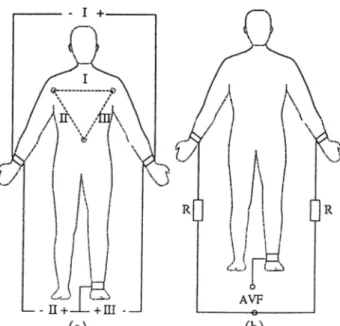
1.1 The acquirement of a. bipolar .signals, b. A V F lead signal. . . . 3

1.2 Precordial lead system... 4

1.3 The Wilson Terminal of augmented and precordial leads... 4

1.4 The waveform and the intervals of the ECG... 4

1.5 AZTEC representation of an ECG waveform... 8

1.6 Application of SAPA technique to an ECG data segment... 10

2.1 4 branch Sub-Band Coder structure. 14 2.2 Sub-band signals at the outputs of analysis bank of the QMF. 15 2.3 Detailed block diagram of the coder in SBC branch A. 16 2.4 The relationship among compression ratio and a. scaling factor, b. threshold... 17

2.5 Frequenc}' responses for Hi[u>) and Eh{u;) filters... 18

2.6 Original and the reconstructed ECG signals with CR=5.7 and P R D = i m ... 19

3.1 8 lead ECG compression structure. 21 3.2 8 x 8 KL transform matrix. 23 3.3 The general block diagram of the compression method for trans­ form sequences with low energy... 25

3.4 Magnitude response of the Lagrange Filter... 26

LIST OF FIGURES IX

3.5 C R versus A P R D for raw ECG data... 28 3.6 The normalized variances of KLT and DOT coefficients... 29 3.7 Magnitude of the frequency response of 33-tap Parks-McClellan

F IR filter with a cut-off 30 Hz... 30 3.8 C R versus A P R D for the 30 Hz low pass filtered data... 31 3.9 C R A'ersus A P R D for the 125 Hz low pass filtered data. 32 3.10 Data set for the ECG compression algorithm. 33 3.11 Characteristic KLT vectors of the given ECG data. 34 3.12 The original and the reconstructed EGG leads, /, I I , VI and V2,

for the case of raw data, usage. CR{DCT) = 6.17, A P R D = 6.19%... 35 3.13 The original and the reconstructed leads, H3, T4. V'5 and VQ for

the raw data usage. CR {DCT) = 6.17, A P R D = 6.19%...36 3.14 The original and the reconstructed leads, I, I I . VI and V2 for

the 30 Hz low pass filtered data usage. CR{DCT) = 8.69,

A P R D = 3.41%. 37

3.15 The original and the reconstructed leads, H3,1'4, У5 and V6 for the 30 Hz low pass filtered data usage. CR[DCT) = 8.69,

A P R D = 3.41%. 38

3.16 The original and the reconstructed leads, 1,11, VI and V2 for the 30 Hz low pass filtered data usage. CR[DCT) = 10.0,

A P R D = 5.77%. 39

3.17 The original and the reconstructed leads, F 3 ,l 4, H5 and V^6 for the 30 Hz low pass filtered data usage. C R \D C T ) = 10.0,

2.1 Coefficients of the QMFB L PF... 18 2.2 Compression ratios and PRD values for different schemes... 19

3.1 Lagrange Filter coefficients. 26

3.2 Performances of various compression schemes. 28 3.3 Coefficients of the 30 Hz FIR low pass filter... 30 3.4 Performances of various compression schemes in 30 Hz low pass

filtered data usage... 30 3.5 Coefficients of the 125 Hz FIR low pass filter. 31 3.6 Performances of various compression schemes in 125 Hz low pass

filtered data usage... 31 3.7 Execution periods of sub-blocks of 8 lead ECG compression

scheme on an IBM XT compatible computer with a mathem at­ ical co-processor, (no.of sam ples= 1024)... 32

B.l Codetable for the amplitude values... 45

B.2 Codetable for the zero runlengths.,· 46

B .3 Codetable for the amplitudes of the SBC branch B... 47 B.4 Codetable for the amplitudes of the SBC branch C... 47 B.5 Codetable for the amplitudes of the SBC branch D... 48 B .6 Codetable for the zero runlengths of the SBC branches B, C,

and D. 48

LIST OF TABLES XI

In tr o d u c tio n

The electrocardiogram (ECG) is a graphic representation of the electrical ac­ tivity of the heart. ECG is recorded from the body surface and it assists an experienced interpreter in giving a prognosis. Recently, digital ECG systems have been widel}·' used in clinical practice. The reasons behind the demand of digital processing of ECG signals can be summarized as follows;

• Recent developments in very large scale integration (VLSI) technologies make it possible to achieve higher volumes of storage media with trifling prices. Memory chips with higher capacities are getting cheaper and cheaper day b}'· day. It is evident th at digital storage of ECG data will be dominant in sup­ plying the memory requirements in near future.

• Expert .systems to interpret digital ECG signals are widely utilized in practice. Digital storage eliminates the need to convert data between analog and digital environments.

• Digital storage is insensitive to the problems of analog recording such as deterioration of signal fidelity in time. This is a problem of databases where ECG recordings of a patient are stored for further comparison or evaluation.

• Digital processing allows development of algorithmic procedures to remove undesired waveforms embedded in electrocardiograms, such as 50-Hz power line interference and baseline drift. Also, some cost effective analysis (e.g., rhythm analysis) algorithms can be implemented in a simple way. Data compression is very effective in increasing the efficiency of automatic computer analysis of electrocardiograms.

CHAPTER 1. INTRODUCTION

Compression of digital ECG signals has been a research topic dne to the de­ velopments in the techniques of digital processing of analog signals [1]. By the usage of digital signal processing to interpret, store or transmit ECG signals, a need to have memory chips with large capacities has arisen. For example, a Holter recorder ^ needs a 1555.2 Mbits of memory for the storage of 24 hours, 3-lead data sampled at a rate of 500 per second with 12 bit resolution. This makes the compression of digital ECG signals a necessity. Some other problems of practical usage can be summarized as below.

• It is reported that transmission of electrocardiograms in the form of ana­ log signals (e.g., FM modulation) over telephone lines has noise problems [2]. Digital transmission is less susceptible to noise than an analog signal. How­ ever, in order to meet bandwidth restriction of the existing telephone lines, a compression algorithm is needed before transmission.

• ECG data volume is increasing linearly every t'ear [3]. In order to make sensible use of this large amount of data (such as serial comparison between old and recent ECG records) efficient data base management systems are manda­ tory. The storage of cardiograms in a digital, easily reached, compressed form from which the original waveforms can be readily reconstructed appears at­ tractive.

Due to the reasons above, compression of the electrocardiograms has be­ come a necessity during the past three decades. In the following sections, we briefly review electrocardiography from an engineering perspective and in­ troduce presently used ECG coding methods. In chapter 2, we present the method for the single lead digital ECG compre.ssion. Chapter 3 introduces the new multilead ECG compression technique.

1.1

E C G W aveform and Standard Lead S y ste m s

In ECG nomenclature, the potential differences between predetermined points of the body are called ECG leads. Different lead configurations are proposed which are called by the name of it’s inventor, such as Cabrera, Einthoven, Goldberger, Nehb, Wilson, etc. In this study, we shall employ signals from a lead system which is referred to as standard leads. This configuration consists of [4];

^ Holter recorder is a portable equipment, which is used to acquire, store and partially interpret two or three channel ECG signals while the patient continues his daily life.

Figure 1.1: The acquirement of a. bipolar signals, b. A V F lead signal. • Bipolar leads: / , / / , / / / .

• Unipolar leads:

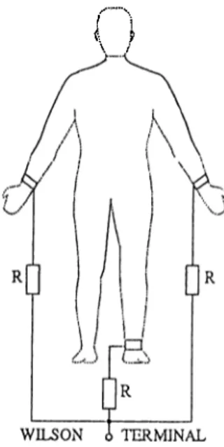
· · Extremity (hands and feet) leads: A V R , A V L , A V F . · · Precordial (chest) leads: y i , . . . , U 6.

Bipolar derivations are the standard frontal plane leads (Fig.1.1.a). They are recorded by measuring potential differences between right arm, left arm, and left leg. This configuration is called Einthoven triangle. The other frontal plane leads, extremity leads (also called as Goldberger leads), use an exploring positive electrode to measure potentials of the right arm (AVR)·, left arm (AVL), and left leg {AVF) (Fig.l.l.b). To obtain one of these signals, following procedure is utilized; first, the other two extremities are connected to each other through ecjual resistances. The mid-point of these resista.nces is used as a reference point. The value of the exploring electrode voltage with respect to that reference will be 1.5 times larger than the original, and therefore called the augmented leads. Second group of unipolar leads, i.e., precordial leads, consists of horizontal chest leads and represents voltage differences between the six chest electrodes and Wilson Terminal (Fig. 1.3). The Wilson Terminal is the central point of connections of three extremity leads through equal resistances. Correct placement of these leads is necessary for correct interpretation, e.g., reversal of the leads causes mirror images in the recordings. A standard ECG recording begins with leads I, I I , I I I . This is followed by A V R , A V L , and A V F , and then the chest leads from VI through V6 [4].

CHAPTER 1. INTRODUCTION ₄

I 1 _{\ /}

Figure 1.3: The Wilson Terminal of augmented and precordial leads.

Standardization of the ECG recordings is a provision for proper interpreta­ tion of these signals. If this is not maintained there may be a serious deficiency in diagnostic value of the recording.

Basic form of an ECG signal is given in Fig.1.4. Duration and amplitude information are valuable for physicians, so that the defects of the heart in cardiac cycle can be determined. Voltage of upward deflections is measured from the baseline to the peak of the wave and that of downward deflections from the baseline to the lowest point of the wa\'e [5].

Before storage, some redundant information can be remo\'ed from ECG recordings by considering inter-channel dependencies. The relationship among ECG signals can be summarized as;

I l l = I I - I (1.1)

A V R = ^ ( / + I I ) (1.2)

A V L = I - i I - (1.3)

A V F = 1 1

-2 (1.4)

This means that storing the leads, I and I I , is sufficient for the retrieval of I I I , AVR, AV L , and A V F signals [6].

1.2

ECG C o m p ressio n T echniques: A R e v ie w

Various compression methods have been proposed to increase the efficiency of the discrete-time systems during storage and transmission [7]. All these methods are aimed to achieve maximum data volume reduction without losing clinically significiuit information. ECG compression methods can be roughly classified into two categories [8];

(i) Direct data compression techniques,

(ii) Transform domain compression techniques.

Direct ECG data compression schemes include .AZTEC, TP, CORTES, Fan and SAPA, DPCM and entropy coding. In this section, these schemes will be reviewed together with a brief description of transform domain compression techniques.

1.2.1

D e fin itio n s o f C o m p ressio n R a tio and R e c o n s t­

r u c tio n Error

CHAPTER 1. INTRODUCTION (

The aim of data compression techniques is to achieve highest compression ratio while minimizing the reconstruction error. During the evaluation of a compression technique, two parameters are considered. These parameters are the compression ratio (CR) and the reconstruction error. The C R is defined as:

C R = 71 ■ b

m (1.5)

where n is the number of samples in the original data, b is the resolution bits and m is the resulting compressed data in terms of bits. This ratio is valid for the comparison of compression methods for data storage. Another CR definition is given for transmission purposes.

Total number of bits per block before compression

C R = (1.6)

Total nu7Tiber o f bits per block a f te r compression

Various criteria have been used in the literature to evaluate the qualit)'· of reproduced signals [9].

(a) M ean S q u a re E rro r (M SE):

The MSE of a sequence with sample length N is given by the average value of scpiares of amplitude differences between the original and the reconstructed signals.

M S E — (^’°rg(tt) ~ ^rec{‘>^)y (17) where Xorg{'>'‘·) is the original data sequence, Xrec(tt) is the reconstructed data sequence, and N is the number of samples.

(b) N o rm alize d M ean Sciuare E r ro r (N M S E ):

The NMSE includes a normalization factor to remove the effect of energy of signal in the error measure,

!'orfl(^t) 3^rec(ti)) Q\

.N-1 ^ ^ M M q /r — ^n=0 Xrec{n)y

E S virgin) (c) R o o t M e a n S q u are E rro r (R M S E ): The RMS error calculation is defined as;

R M S E =

En

=0

(•'^org(^)

EnEo^ virgin)

(d) P ercen t R oot M ean Square Difference (P R D ):

The PRD is the most widely used quantitative measure of distortion in ECG data compression. It is defined as;

P R D =

i

y^r.=n \^orgip) ^'í^rec(^)]^ * 100 ( 1 .1 0 ) Since resulting error depends not only on the absolute difference but also on the offset of the signal, special attention must be paid when using the PRD [10]. A small persistent error on the P-wave or baseline changes the PRD value more than a larger error on the ORS comple.x.

(e) A verage Percent Root M ean Square D ifference (A P R D ):

This measure of quality is used for the evaluation of multichannel ECG compression schemes. In order to calculate the average PRD, an algorithm processes each of the original ECG channels and the PRD is calculated for all output sequences. The average of all PR D ’s gives APRD [9].

1.2.2

D ir e c t E C G D a ta C o m p ressio n T ech n iq u es

Direct ECG compression methods can be classified into three groups, i.e., toler­ ance comparison data compression techniques, data compression by differential pulse code modulation and entropy coding.

I. T o leran ce C o m p ariso n D a ta C o m p ressio n T ech n iq u es

Tolerance comparison data compression techniques employ polynomial pre­ dictors and interpolators. The main idea behind the polynomial predictors/in- terpolators is to approximate the samples within a predefined aperture by a line where only the line parameters (e.g., length and amplitude) are saved. This results in the elimination of the samples which can be implied b}^ examining preceding and succeeding samples. Zero-order predictors and interpolaters are the simplest types of this group of techniques.

I.(a) T h e A Z T E C T echnique: The Amplitude Zone Time Epoch Coding (AZTEC) originally developed by Cox et al. [11] as a preprocessing program for real-time monitoring of electrocardiograms. It has proven to be useful for automatic analysis functions such as QRS detection, but is inadequate for visual presentation of the data.

CHAPTER 1. INTRODUCTION

Figure 1.5: AZTEC representation of an ECG waveform.

Let Vi be the sample of a digital ECG waveform, v^ax and are the maximum and minimum values, respectivel}^, of the set {ui}o^ where i ranges from 0 to m. As long as the difference between the limits, {v^ax — Vmin), does not exceed an experimentally determined threshold, the fluctuating voltage till is considered to be adequately represented by a constant voltage, or line, midway between the limits. When finally a sample would necessiate seperating the limits by more than the threshold, the preceding average of the two limits is stored in the memory and Ccdled the value of the line. Also, the time since the limits were initialized, is stored as duration of the line. When a signal of higher frequency and amplitude such as the QRS begins, the voltage of samples will change rapidly, and lines of short duration will be formed. A series of lines, each containing four samples or less, is considered to be adequately represented by a constcuit rate of voltage change, or slope, as long as the voltage difference between adjcicent lines does not change sign. The slope duration and the voltage between the lines bounding the slope are stored as the next pciir of data words.

The complete AZTEC method can be summarized as the ordered set of lines and slopes. A typical AZTEC representation of an ECG waveform is shown in Fig.1.5. Even though it produces a high compression ratio (10:1, 500 Hz sampled data with 12 bit resolution), the reconstructed signal fidelity is not acceptable to the cardiologist because of the discontinuous nature (step-like quantization) of the reconstructed ECG waveform.

reduction algorithm [12] was developed for the purpose of reducing the sam­ pling frequency of an ECG signal from 200 to 100 Hz without diminishing the elevation of large amplitude QRS’s.

The algorithm is based on analyzing the trends of sampled points, hence, it processes three data points at a time; a reference point (Xo) s,nd two con­ secutive data points (Xi and X^) [8]. Either X i or X2 is to be retained. This

depends on which point preserves the slope of the original three points. TP retains peak and valley points at which the sign of the signal changes or turns (i.e., the turning point). The algorithm iDroduces a fixed compression ratio of 2:1 where the reconstructed signal resembles the original signal with some distortion. In [8] for 200 Hz, 12 bit sampling conditions, P R D is given as 5.3%. .A. disadvantage of the TP method is that the saved points do not represent ecpially spaced time intervals (asynchronous). In such a case some bits are needed for timing definition.

I.(c ) T he C O R T E S T echnique: The Coordinate Reduction Time En­ coding System (CORTES) is a hybrid of the turning point and AZTEC algo­ rithms that is designed to take advantage of the strong points of both methods [9]. The CORTES simultaneously applies AZTEC to the isoelectric region and T P 'to the clinically significant higher frequency regions (e.g., QRS complex, P and T waves) of the ECG signal. It uses an experimentally determined line length threshold. Tin- Once an AZTEC plateaue - is produced, CORTES saves the AZTEC data if the plateau is longer than Tin or it saves the TP data if the plateau is shorter than or equal to Tin- Once AZTEC plateaus are generated, no slopes are produced. CORTES in-ovides nertrly the same data reduction rate as AZTEC with approximately the same reconstruction error as TP. The comiDression ratio of CORTES is reported as 4.8 for 200 samples per second with 12 bit resolution, giving a PRD of 7.0 percent.

I.(d ) Fan an d S A P A T ech n iq u es: Fan and Scan-.Along Polygonal Ap­ proximation (SAPA) algorithms are heuristic methods for piecewise-linear ap­ proximation of functions of one variable and use upper and lower bounds on the absolute value of error to minimize the number of approximating segments subject to that error limit [13] [14] [15].

Fan and SAPA techniciues both have the same objective, to replace the signal by straight lines within aperture e. [16] claimed that the Fan and the SAPA-2 (a modified version of SAPA) are equivalent. So, we are contented with the review of the SAPA-2 algorithm.

CHAPTER 1. INTRODUCTION 10

Figure 1.6: Application of SAPA technique to an ECG data segment. The nonredundant (reduced data) samples are called vertices. When be­ ginning the approximation algorithm, the first data point is a vertex. Upon reception of a later sample at discrete time instant, k=c, the normalized slopes of the two lines joining w{s) to w{c) -b e and to io[c) — e are calculated. Here, w[k) corresponds to the original sampled data which will be approximated. The slopes are;

and as indicated in Fig. 1.6. + e - w { s ) c — s ( 1 . 1 1 ) J. w ( c ) — c — t u ( s ) Lf — c — s ( 1 . 1 2 )

As each new data point is processed, the current smallest value of U is stored as mi, and the current largest value of L is stored as m 2. The numbers mi and m 2 thus store the maximum and minimum slopes that a line from s ma3' have and still pass within ±e of subsequent data points. Whenever

m-2 > mi (1.13)

cis is the situation in Fig.1.6 at k = c 3, the immediately previous data is selected as a vertex and the preceding samples between two consecutive vertices are discarded.

The SAPA output is represented by the reduced data

(k,w{k)) , k - s , , S 2,... ( U 4 )

where iu{k) is amplitude of the vertex at time instant k. During reconstruction, the data between any two vertices is approximated by points on the straight

line joining the two vertices. SAPA-2 improves the efficiency of the algorithm by testing an extra slope, E. It is defined as

E w{c + z) — w(s)

c + i — s (1.15)

and aims to test whether or not the points between k = s and k = c + i may be adequately approximated by a straight line. If the line for i = S with slope E does not pass through the shaded area of Fig.1.6, then the data at /: = c + 2 is a vertex. [8] reports a compression ratio of 3.0 for both Fan and S.A.PA algorithms with a PRD of 4.0 percent for 250 Hz, 12 bit sampling conditions.

II. ECG D a ta Com pression by D P C M

Differential pulse code modulation (DPCM) is the well-known data coding technique in which main idea is to convert the actual correlated signal into an uncorrelated signal. Compression is achieved by coding the estimation error sequence which has smaller variance than the original signal. There exists both lossless and lossy DPCM compression methods. The estimator of a DPCM coder can be any estimation algorithm such as polynomial or linear predictors [3]. The highest compression ratio for this category has been reported as C R = 7.8, P R D = 3.5% for 8 bit resolution and 500 Hz sampling frequency [8].

III. Entropy C oding

Data compression by entropy coding is obtained by means of assigning variable-length codewords to a given quantized data sequence according to the frequency of occurrence. Huffman coding is a popular method of construct­ ing variable-length codes which assigns shorter(longer) code lentghs to values occuring with higher(lower) probabilities [17]. In practice, entropy coders are used together with the other coding techniques, e.g., estimation error sequence of DPCM is coded by considering distribution of amplitude values.

1.2.3

T ransform D o m a in C om p ression T ech n iq u es

The rationale of transform domain compression techniques can be summarized as; (i) representing tim e domain signal by a set of orthononnal basis functions and (ii) discarding a group of transform coefficients to achieve data volume reduction. .A.S it can be expected, the basis functions with the low coefficient

variances are discarded while the ones with the large values are retained. This process of component selection is called as variance criterion [18].

CHAPTER 1. INTRODUCTION 12

Various transform domain compression techniques are proposed for EGG signals. Among these, Karhunen-Loeve (KLT) expansion is the optimum trans­ form with respect to mean-square error criterion [19] [20]. Minimizing mean square error indicates that for a given value of error, KLT needs the least num­ ber of orthonormal functions to represent the input signal. However, there is no fast algorithm for computing KLT or it ’s inverse. So, some sub-optimum but practical transforms such as Fourier (FT) [21], Discrete Cosine (DCT) [18][22], Walsh (WT) [22] [23], Haar (HT) [18], etc., are used for coding EGG signals. Although compression ratio of suboptimum transforms are lower than KLT, relatively small amount of computing effort rnahes these methods advan­ tageous. These transformation compression techniques have been employed in compressing two or three EGG channels.

S in gle L ead E C G D a ta C om p ression

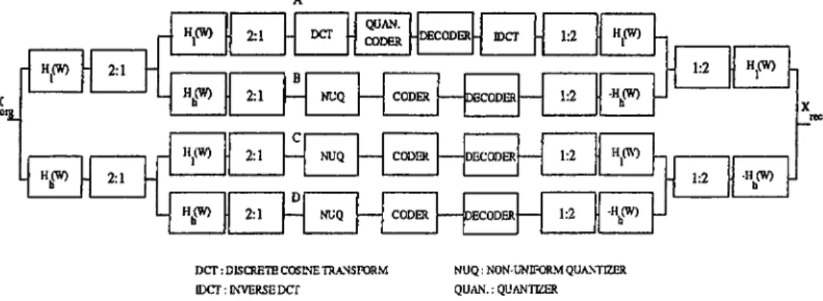
In this section, we present a sub-band coding (SBC) based compression scheme for ECG signals. Sub-band coding has been successful!}^ applied to speech [24] and image coding [25] [26]. In the coding of sub-band signals, one takes the advantage of the nonuniform distribution of energy in the frequency domain to judiciously allocate the bits to represent the sub-band signals. In our method the subsignal with the lowest frequency content is encoded by using a discrete cosine transform (DCT) based compression scheme [27] and the other sub­ signals are quantized using deadzone quantizers. The resulting data is coded using runlength coding of zero valued samples and variable length coding of the nonzero samples. In the next section, a detailed description of the new procedure is given.

2.1

D e sc r ip tio n o f th e p roced u re

The whole structure which is used to compress ECG signals is given in Fig.2.1. The single lead ECG signal is decomposed into 4 subsignals by using a quad­ rature mirror filter bank (QMFB) in a tree structured fashion and resulting stages of the tree is decimated by a factor of two. QMFB is one of the building blocks used in multirate signal processing. It finds applications in situations where a discrete-time signal is to be split into a number of consecutive bands in the frequency domain. This division into freciuency components removes the redundancy in the input and has the advantage that the number of bits used to encode each frequency band can be different, so that the encoding accuracy is always maintained at the required frequency bands. In the absence of quantiza­ tion errors, a QMF bank based tree structure provides perfect reconstruction.

CHAPTER 2. SINGLE LEAD ECG DATA COMPRESSION 14 X o;2_ rl Hj(W) 2:1 -HfW) . _2:1 h H (W) _2:1 H^W) _2:1 Hj(W) _2:1 H(W) D 2:1 QUAN. CODER CODER DECODER NUQ NUQ DECODER 1:2 H^(W) 1:2 -H(W)₀ 1:2 1:2 -HfW)_D DCT: DISCRETE COSLNE TR.ANSFORM

IDCT: INVERSE DCr

NUQ: NON-UNIFORM QUANTIZER QU/\N.: QUAN'nZER

1:2 I) H(W)

- 1:2 -H(W) b

Figure 2.1: 4 branch Sub-Band Coder structure. i.e.,

y(n) = x{n — K ) , K an integer. (2-1) where y{n) is the output and x{n) is the input of the QMFB. This is because of the fact [29] that the low pass. and the high pass filter, Hh{ui) satisfy the following condition,

p + I Hk{u) r-= 1

(

2

.

2

)

ECG leads are sampled at 500 Hz. It is observed that energy of the ECG signals is highl}· concentrated at frec[uencies less than 62.5 Hz. The 4 band filter bank is used to assign a coding method to the signals of that frequency range. Each sub-band is encoded according to criteria that are specific to that band. ECG waveforms depict that all the three bands except the lowest frequency band have noise-like variations (Fig.2.2), therefore coded using non-uniform quantizers. After quantization, a code assignment procedure is realized using amplitude and runlength lookup tables which are derived by variable length coding from the histograms of quantized sub-band signals.

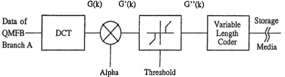
A detailed diagram of branch A coder of the SBC is illustrated in Fig.2.3. Transform coding was used in [18] to compress discrete-time ECG signals. In our method we use a discrete cosine transform (DCT) based transform coding method to compress the sub-band signals with the lowest frequency content. It is observed th at the ECG signal energy is mainly concentrated in the lowest frequency band. Because of this, the lowband signal (branch A) has to be carefully coded. The high correlation among neighbouring samples makes the lowband signal a good candidate for efficient predictive or transform coding. In this study, we have chosen to use DCT in view of the known efficiency of transform codes.

I I---- 1---1----I--- 1---- 1 0 . 0 0 O.fO 1 .6 0 2 .4 0 Time ( s e e . ) A v \ J A v i , ■w\ I I I--- 1--- 1---1---1 0 . 0 0 0 . 8 0 1 .6 0 2 .4 0 Time ( s e c . )

Figure 2.2: Sub-band signals at the outputs of analysis bank of the QMF. The DCT of a data sequence x(n), n=0,l,---;(N-l) is defined as [27];

N - \

(2.3) n=0

= 1,2,..., (iV - 1) (2.4) n = 0

where G(k) is the kih DCT coefficient. The inverse discrete cosine transform (IDCT) of G(k) is given as;

* ) = ^ C ,X 0) + ' ¿ ‘ „ = 0 ,1 .2 ....,{ A '- 1 ) (2.5)

k = l

After the application of discrete cosine transformation with a block size of iV=64 samples to the upper branch, we obtain the transform domain coeffi­ cients, i.e., G{k). If drastic variations occur in the recordings, one can scale the transform coefficients by a factor q, i.e.,

G'{k) = a ■ G{k) (2.6)

In many cases ECG recording levels do not change from one recording to an­ other one.

CHAPTER 2. SINGLE LEAD ECG DATA COMPRESSION 16

G(k) G’(k) G”(k)

Alpha Threshold

Figure 2.3: Detailed block diagram of the coder in SBC branch A. Gf(0) is the DC value of the sample block. The quantization of the G(0) coefficient performs a DC level difference between the blocks of data. So, G(0) is not quantized. G'(0) is located at the beginning of each coded block and represented by fixed length 13 bits.

Bit assignment of transform coefficients can be realized bj'^ the relationship (see Appendix A);

4 ^max

7T

^ G ( ^ k ) r a a x ^ ^^y^^max ? k — ₀, .₁, ₁ (2.7)

The other elements of the data stream is thresholcled by the succecling block. This operation is called as threshold coding and defined as retaining the coeffi­ cients whose magnitudes are above a preselected, threshold {¡3) and discarding the others.

' G'{k) - 13 i f G'{k) > 13 G' \k) =

0 otherwise

The subtraction of ß from the G'{k) values which are greater than ß, squeezes the d}'namic range of the amplitude values. Hence, the discontinuities at the histogram of amplitudes are removed.

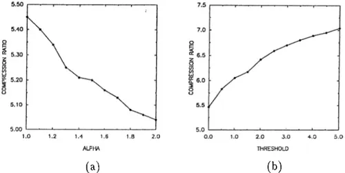
The scaling and thresholding operations serve for the control of compression ratio and error in the reconstructed seciuence. The dependency of compression ratio to these two parameters are shown by experimental values in Fig.2.4. The error of the reconstructed sequence is also inverse proportional with cv and direct proportional with ß. These operations are followed by the quantization of the transform coefficients.

Since resulting error is very sensitive to quantization, only a floating point to integer conversion is applied, i.e.,

G"'[k) = {G''{k)) (2.8)

(a)

(b)

Figure 2.4: The relationship among compression ratio and a. scaling factor, b. threshold.

be achie^'ed as;

= / (™')(G"(i-) + 0.5) i f G"(k) > 0 — 0.5) otherwise

The nonzero and zero values of G"'(A;)s are coded by amplitude and runlength lookup tables, respectively. These tables are derived by applying Huffman Cod­ ing algorithm to the probabilities estimated from histograms of coefhcients. It is reported in [28] that DCT coefficients in images exhibit a Laplacian type am­ plitude distribution. We observed empirically thcit distribution of amplitudes in DCT domain can be approximated by Laplacian probability density function for ECG signals. The corresponding code tables are attached in Appendix B.

The bit streams which are obtained from coding of 4 sub-bands are multi­ plexed and stored. Reconstruction begins by decoding the bit streams of A, B, C and D branches. Considering the coding algorithm of the analysis part, an appropriate decoder is assigned to each branch. The 4 branch synthesis bank has the dual operations of the analysis part.

2.2

S im u la tio n resu lts

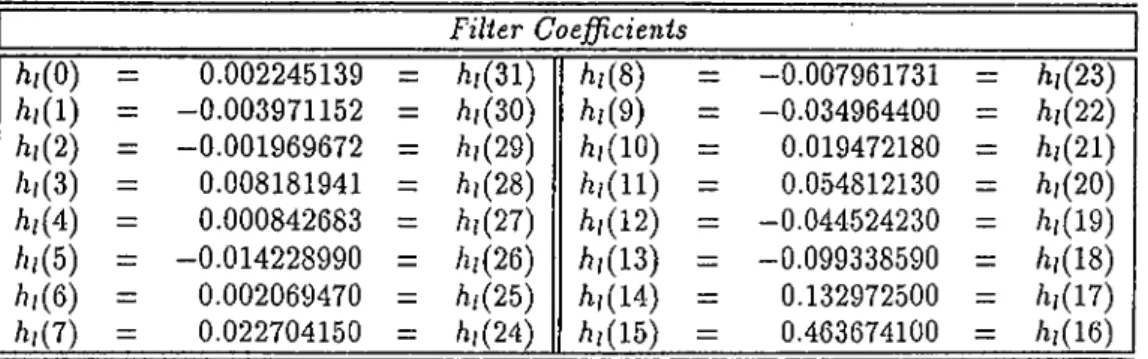
The ECG signal is sampled at 500 Hz with 12 bits resolution. The discrete time ECG signal is partitioned into blocks with lengths of 1024 samples each. A 32-tap finite impulse response QMF pair which is described in [29] is used in the sub-band decomposition structure. The coefficients of the lowpass filter, /i;(n), are given in Table.2.1. The highpass filter coefficients are determined

CHAPTER 2. SINGLE LEAD ECG DATA COMPRESSION 18 Fi l i e r C o e f ß c i e n i s h , m = 0.002245139 = /i,(31) h i { 8 ) = -0.007961731 = /1,(23) h , { l ) = -0.003971152 = /i,(30) h i { 9 ) = -0.034964400 = /1,(22) h, { 2) = -0.001969672 = /1,(29) /ii(lO) = 0.019472180 = /1,(21) /11 (3) = 0.008181941 = /i,(28) /1,(11) = 0.054812130 = /,,(20) h , 0 ) = 0.000842683 = /1,(27) /1,(12) = -0.044524230 = /1,(19) /ii(5) = -0.014228990 = /i,(26) /1,(13) = -0.099338590 = /1,(18) /11(6) = 0.002069470 = /1,(25) /1,(14) = 0.132972500 = /1,(17) /1,(7) = 0.022704150 = /,,(24) /1,(15) = 0.463674100 = /1,(16)

Table 2.1: Coefficients of the QMFB LPF.

Figure 2.5: Frequency responses for i-/;(uj) and filters. simply as

hh{n) = i - i r ■ hi{n) (2.9) i.e., the highpass frequency response is the shifted version of the lowpass fre­ quency response by an amount of tt (mirror image relationship). These FIR. filters of Fig.2.5 approximate the perfect reconstruction condition 2.2 and also satisfy the following bounds:

0.9943 <1 -t- I

Ih{u})

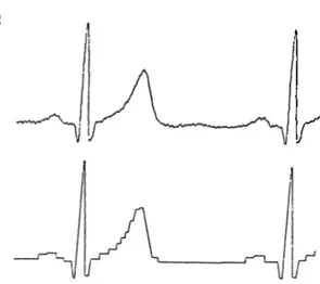
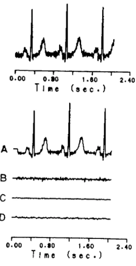
|^< 1.0058 (2.1 0)

Discrete cosine transform with a block size of 64 samples applied to branch A and the other branches, B.C. and D, are coded employing quantizers of 7, 3 and 3 levels, respectively. As it is reported in Table.2.2, the compression ratio {CR) is determined as 4.6 and the PRD is 3.2%. Also higher compression ratios as 5.7 obtained with a PRD=7.0% and we observed that it is visually impossible to distinguish the original and the reconstructed signal as shown in Fig.2.6.

We also applied DCT coding method to the input ECG signal without per­ forming any sub-band decomposition, e.g., for a,CR of 4.6, PRD is determined

METHOD CR PRD DCT 4.2 4.3% DCT 4.6 4.8% SBC-hDCT 4.2 2.6% SBC+DCT 4.6 3.2% DCT,filtered data 4.5 2.1% DCT,filtered data 5.3 2.9% SBC+DCT,filtered data 4.5 1.7% SBC+DCT,filtered data 5.3 2.6%

Table 2.2: Compression ratios and PRD values for different schemes.

Figure 2.6: Original and the reconstructed ECG signals with CR=5.7 and PRD=7.0%.

as 4.8%. Whereas the sub-band coding method produces a PRD of 3.2% for the same CR.

As it is seen in Fig.2.6, the ECG data is corrupted by EMG noise A low pass filter with a cut-off frequency equal to 125 Hz. is used to remove noise components and CR and PR D of 5.3, 2.6% are obtained respectively.

Simulations have been completed on a personel computer and it is observed that SBC algorithm works 2.5 times faster than the conventional DCT based compression technique. .Also, the SBC structure can be very conveniently implemented by digital signal processors which have special macros for the simplification of filtering and FFT algorithms.

^Wlien the patient contracts his muscles during the acquisition of the ECG data, an additive noise called Electromyogram (EMG) noise is produced on the ECG recordings.

C hapter 3

M u ltich a n n el E C G D a ta C om p ression

This chapter presents a data compression method for digital multilead elec­ trocardiogram (ECG) signals. A linear transform is applied to samples of the eight standard ECG lead signals. In this way the correlation among the ECG channels are aimed to be reduced. The resulting uncorrelated transform do­ main signrils are compressed using various coding methods, including multi-rate signal processing and transform domain techniques. In the proposed scheme higher compression ratios are achieved compared to the single channel com­ pression techniques because the inherent correlation among the ECG leads is exploited in this multichannel approach. The resulting technic|ue is also com­ putationally efficient.

3.1

D e sc r ip tio n o f th e P roced u re:

The block diagram of the multichannel compression method is shown in Fig.3.1. The 8 lead ECG signals are first passed through a preprocessor. The function of this block is to prepare raw ECG data for further processing. After pre­ processing the input signals, the resulting discrete-time sequences are linearly transformed to another set of sequences. I'he aim of this process is to decorre­ late the highly correlated ECG signals. The transformation matrix, / 1, can be the matrix of the optimum transform, Karhunen-Loeve Transform, or any of the suboptimum transforms such as Fourier Transform, Discrete Cosine Transform, Walsh Trcvnsform, etc. The rationale of the compression method is to apply different coding schemes to uncorrelated transform domain sequences. The se­ quences with high energies, yo, are coded by sub-band coders (SBC’s) as in Chapter 2. The sampling rate of the other transform sequences (ys,···,^?) are reduced by a factor of 4 and the downsampled sequences are compressed by

n VI V2 V3 X 0 G SB _{/ /} SB G X 0 ____J________ CODER ₎₎ DECODER _, X 1 y y ’ X 1 SB _{/ /} SB , X 2 CODER )) DECODER X 2 LINE\R INVERSE X 3 TRA.SS. TRANS. X3 PRE- _-1 POST PROCESS X 4 A A X 4 PROCESS X 5 V X 5 DC _{/ /} DECODER , X 6 CODER )) INT X6 V V ' . X 7 DC _// DECODER X 7 CODER ₎₎ INT .VI· SBC: SUB-BAND CODKR D C : DliCIMATOR INT: INTHRPOLATCR

Figure 3.1: 8 lead ECG compression structure.

a DCT coding method. Bit streams at the outputs of coders are multiplexed for the storage purpose.

Reconstruction needs a reverse process of the encoding steps. SB coded sequences are reconstructed by using SB decoders as described in Chapter 2. The decimated and transform coded sequences, i.e., y5,....yr, are decoded by

inverse transform domain operations and the resulting samples are interpolated by a factor of 4. Inverse of the transform matrix, A~'·, is applied to decoded sequences to get back to the time domain. The side information of the prepro­ cessor (only two bits) is also stored with the compressed data block and used for the proper demultiplexing of reconstructed data. The detailed description of the compression algorithm is given in the following sections.

3,1,1

T h e P rep ro cesso r

The preprocessor changes the orders of the ECG channels. The aim of the preprocessor is to bring highly correlated channels close to each other.

The six precordial (chest) leads, i.e., R l , ..., V6, represent variations of the electrical heart vector amplitude with respect to time from six different narrow angles. During a cardiac cycle, it is reasonable to expect high correlation among precordial leads.

CHAPTER 3. MULTICHANNEL ECG DATA COMPRESSION 22

energy values. The two horizontal lead waveforms (J and I I ) which have relatively less energy contents with respect to precordial ECG lead waveforms are chosen as seventh and eighth channels.

The aim of the reordering the ECG channels is to increase the efficiency of the linear transform which is described in the ne.xt subsection.

3 .1 .2

T h e L inear T ransform er

The outputs of the preprocessor block are fed to the linear transformer. In this linear transform block, the reordered ECG channels are linearly transformed to another domain.

Let xic{m),k = 0 ,1 ,...,// — 1{N is equal to eight in our case), be the reordered ECG signal samples at discrete time instant m, the transform domain samples at time instant m are given by;

Yn. = A - X, (3/1)

where K. = [j/o(m) , = [ x o ( m ) , a n d A is an N X N matrix.

In this work, we used both optimum (Karhunen-Loeve) and suboptimum (Discrete Cosine) transforms for the m atrix /1.

(a) K arhunen-Loeve Transform

Karhunen-Loeve Transform (KLT) is the optimum linear transform for the decorrelation of input sequences. The discrete KL transform miitrix is con­ structed from the eigenvectors of the covariance matrix of the input data (G\')· It is known that such a matrix reduces C-x to it's diagonal form, i.e..

Cy

=

A'^CxA = diag{Xk}

,

Xk ■ kX''tigcnvalue of Cx- (3.2

which indicates that application of the KLT to a set of random variables results in uncorrelated random variables.

KLT matrix depends on the signal statistics. The transform matrix has to be updated for unstationary inputs. In practice, ECG signals can not be con­ sidered to be wide sense stationary random processes. However, we examined

Л -KLT = ■ 0.1883 0.1568 0.4199 0.4874 0.5024 0.4509 0.2615 0.0452 ■ -0.1779 -0.1707 -0.3426 -0.2350 -0.0552 0.3290 0.6821 0.4360 0.3715 0.5210 0.0591 -0.1347 -0.3928 -0.0400 0.4749 -0.4331 -0.2164 0.7699 -0.4322 0.1633 0.0982 0.0392 -0.2231 0.2934 -0.8073 0.0066 0.0553 0.1945 -0.0723 0.1165 0.1529 -0.5149 -0.2528 0.2391 0.4301 -0.4758 0.4233 -0.4700 0.2042 0.1609 -0.1722 0.0805 0.5204 0.2431 -0.6256 -0.0420 -0.0233 0.4902 0.0522 -0.1359 -0.2392 0.5823 0.0699 -0.6702 0.3543 0.0544 .

Figure 3.2: 8 x 8 KL transform matri.x.

blocks of data that are processed for the factors which corrupt the stationarity of the ECG signals (e.g., beiseline drift of the ECG signals is removed).

We observe ECG data for short periods of time. Hence, time averages take the place of the expectation operation. The covariance matrix of the input data can be approximated by the eciuation;

. Л/-1

1=0

xo(0

[а;о(г) · · · д;дг_1(г)] (3.3)

where M is the number of samples within a block of data and N is the input size of the KLT. KLT matrix of Fig.3.2 is obtained by such an approximation of the covariance matrix of the signals given in Fig.3.10. The rows of that matri.x is constructed from the ordered eigenvectors of Cx by considering the abso­ lute magnitudes of the corresponding eigenvalues. The uncorrelated transform domain sequences are shown in Fig.3.11.

KLT results in optimum decorrelation of the input data. But, it is com­ putationally inefficient. For that reason, suboptimum transforms are proposed which have close performance to KLT. Such a linear transformation will be given in the next section.

(b) D iscrete Cosine Ti'ansform

We also used DCT as a linear transformer. DCT matrix approximates KLT in the case of high correlation [30] among input signals and there are com­ putationally efficient algorithms to implement the DCT [31]. A definition of the DCT of a vector was introduced in Chapter 2. A new DCT definition can be given for the comparison of KL and discrete cosine transformations with respect to their energy compaction properties. The new definition of the DCT

CHAPTER 3. MULTICHANNEL ECG DATA COMPRESSION 24 is given as follows: N - l ■ N- i G'(0) = - L = x { n ) { 2 n H- 1)кт = V ^ £ v - * = 1 . 2 , (ЛГ - 1) 7 1 = 0

whereas ГОСТ is given as follows: ■N-l x{n) = (3.4) (3.5) « = 0 , 1 ,2 ,,..,( Л - 1 ) (3.6) The above DOT definition is just a scaled version of the one in Chapter 2. VVe introduced this new defiirition to compare the normalized variances of trans­ form domain vectors resulting from KL and Discrete Cosine Transforms.

3.1.3

C o d in g o f th e T ransform D o m a in Signals

We observed that the energy of the linearly transformed signals decrease while their subscripts increase. This is due to the linear transformer which decorre­ lates the input signals, Xi{n)^ i = 0 ,..,7 (Fig.3.1). The transform domain se- cpiences, yo{'n)·, are faithfully compressed by using the SBC described in Chapter 2. We also observed uhat, y s i n ) , 2/7(71) have little energy and the}'^ carry little information. These transform domain sequences are decimated by a factor of four and coded in the DCT domain. The description of the com­ pression methods will be given in the next subsections.

(a) Sub-band Coder

We want to code the signals, 7/0(72),.., 7/4(77), in an accurate way. High quality coding of ECG signals can be carried out using SBC’s [32], therefore we selected the SBC to code the transform domciin sequences, 7/,(?i), i — 0, ..,4, which are high energy signals compared to the 7/5(22), 7/6(?*) ¿tnd 7/r(?^).

After sub-band decomposition of any yi{n), {i = 0,.., 4), one of the resulting subsignals is coded by the DCT method as described in Section.2.1. The desired compression ratios with the expense of PRD values can be attained by properly setting the quantizer levels of the DCT coders. The other three subsignals are non-uniformly quantized. Reconstruction block of the Section.2.1 is used at the decoder.

LP F : LOW PASS FIL'l'ER

Figure 3.3: The general block diagram of the compression method for transform sequences with low energy.

Simpler methods can be used to code low energy signals, .., yr{n). Such a method is introduced in the next section.

(b) D ecim ator-C oder-Interpolater B lock

The .signals y5{n)^ye{n) and y7{n) can also be coded by using the SBC structure

of Section.2.1. However, we observed that all the subsignals except the sub­ signal at branch A of Fig.2.1 contains very little information when sub-band decomposition is applied to these signals. Due to this fact, we process only the subsignals (lowband signals) at branch A of the sub-band decomposition structures employed to code y5{n), yQ{n) and y7{n).

Since we drop all the highband subsignals in our coding method, we do use only the first branch of the subband filter bank. The first branch consists of a lowpass filter with a cut-off 7t/ 2 and a downsampling block. In multirate signal processing what this branch does is called the digital decimation operation by a factor of two [33].

The 2:1 downsampler performs a sampling rate reduction by dropping every other sample of its input sequence, i.e..

j(n) — ro(2?r) (3.7)

where io{n) and z{7i) is the input and output sequences of the downsampler, respectively. When a digital signal is downsampled, aliasing may occur. In order to avoid aliasing, the input is low-pass filtered before the downsampling operation.

In the decirnator coding structure of Fig.3.3, two successive blocks of deci- mators are used which reduce the sampling rate by a factor of four. We used a seventh order Lagrange Filter which is a half-band filter as the anti-aliasing

CHAPTER 3. MULTICHANNEL ECG DATA COMPRESSION 26 Filter order Filter Coefficients MO) Ml) h{2) M3) h(6) h{6) 7 -1/32 0 9/32 1 9/32 0 -1/32

Table 3.1: Lagrange Filter coefficients.

Figure 3.4: Magnitude response of the Lagrange Filter.

filter of the decimators. The coefficients and the magnitude of the frequency response of this filter are shown in Table.3.1 and Fig.3.4, respectivelj^.

After the decimation by a factor of four the y i { n ) , (i = 5,6,7) signrd, the

sequence is compressed by the coder block. The coding is imiDlemented as in the case of SBC lowest frequency band. The decimated samples are trans­ formed to the DCT domain block by block. As it is stated in Section.2.1, the compression ratio and the reconstruction error can be set to the desired values by adjusting the quantizer parameters, i.e., scaling and thresholding pcirame- ters. The quantized samples are then noiselessly coded by using amplitude and zero runlength lookup tables which are derived by truncated-Hulfman Coding procedure. These tables are given in Appendix B.

Reconstruction of the transform signal begins with decoding the compressed bit stream. A tree-search is needed to convert variable length coded samples to amplitude values. After that, the decoder implements dual operations of the coder. Decoded signals are interpolated by a factor of four.

The digital interpolation is the dual operation of the digital decimation [33]. An interpolate!· by a factor of 2 consists of an upsampler which inserts a zero

between adjacent samples of its input sequence, i.e., v[n) — u(n/2) n = 2k, k an integer

0 otherwise

and a lowpass filter with a cut-off 7t/ 2 . To achieve interpolation by a factor

of four, we used two successive interpolation by a factor of two blocks which employ the same Lagrange Filter used in decimators.

The interpolation by a factor of four concludes reconstruction of the signals, ysin), ..,2/7(7?). The Decimator-Coder-Interpolater algonthm for the low energy signals is computationallj^ more efficient than the SB coding method. This is due to the fact that the DCI method consists of just a single branch of the SBC method and the Lagrange half-band filters use only integer arithmetic. Although this method is less complex than the SBC, the reconstruction ei'ror is very close to the SBC results.

3.2

S im u la tio n R e su lts

The method described in Section.3.1 is realized on the data set which is ac- ciuired by ARS EKG-12K PC add-on card [35]. This data set consists of stan­ dard ECG signals which are introduced in Section. 1.1. The acquired signals are first joreprocessed. The KLT and the DCT are emploj^ed to transform the ECG signals, xo(n),..,.T7(??), in the linear transformer of Fig.3.1. In the case of KLT, the 8 X 8 matrix obtained in Section.3.1.2.(a) is applied and for the DCT, the definition introduced in Section.3.1.2.(b) is used.

The transform domain signals, 2/i(n), i — 0,..,4, are coded by the SBC’s and the signals, .., yr{n) are coded by the DCI block of Section.3.1.4.

The compression ratio (CR) is defined as c ■ n ■ b CR==

m (3.8)

where c and n is the number of channels and number of samples per channel, respectively, b is the resolution bits and rn is the total number of bits at the outputs of the coders. The fidelity measure average percent root mean square difference [APRD] described in Section. 1.2.l.(e) is emploj'edfor the evaluation of the reproduced signals.

If DCT (KLT) is used as the linear transformer then we obtain the cod­ ing results shown in second (third) column of the Table.3.2 for given A P R D

CHAPTER 3. MULTICHANNEL ECG DATA COMPRESSION 28 CR(SBC) CR(DCT) CR(KLT) APRD(%) 4.02 4.97 6.19 3.70 4.07 5.18 6.43 3.84 4.19 5.22 6.62 4.04 4.22 5.23 6.82 4.27 4.31 5.54 7.09 4.57 4.50 6.00 7.71 5.60 4.57 6.08 7.87 5.93 4.65 6.17 7.98 6.19

Table 3.2: Performances of various compression schemes.

Figure 3.6: The normalized variances of KLT and DCT coefficients. values. In the first column of Table.3.2, the C R values for the SB coding of xo{n), ..,X7[n) are given for the same A P R D values. These results are also

summarized in Fig.3.5. Clearly, the new multichannel coding method outper­ forms the single channel SBC method.

The normalized variances.

7 v -l

»■«I = <rV al. (3.9)

fc=0

(where af denotes the variance of the element of the vector, (j) = [^o, <^i? ···- , (^K-\Y) versus the coefficient index of the transform domain secpiences, ?/,(n), i = 0,.., 7, for KLT and DCT are plotted in Fig.3.6.

In the multichannel ECG coding method, if KLT is used as the linear transformer then we get better results in comparison with the case of the linear transformer which emplo3^s DCT. Hoivever , the DCT based linear transformer is more computationally efficient than the KLT based linear transformer.

The ECG signals are filtered to attenuate the high frequency EMG noise with 33-tap equiripple Parks-McClellan FIR filters with cut-off frequencies 30 Hz and 125 Hz. The coefficients and the frequency responses of 30 Hz (125 Hz) filter are given in Table.3.3 (Table.3.5) and Fig.3.7, respectively. The m ulti­ channel ECG coding is applied to the filtered ECG data. Large increases in the C R values are observed and the coding results are described in Table.3.4,3.6 and Fig.3.8,3.9.

Table.3.7 summarizes the timing requirement of different blocks of the com­ pression algorithm. As it is seen, linear direct and inverse transforms consume approximately 26% of the processing time to fully compress and reconstruct 8

CHAPTER 3. MULTICHANNEL ECG DATA COMPRESSION 30 Filter Coefficients m = h (l)= h(2)= h(3)= h(4)= h(5)= h(6)= h(7)=

h(8)=

h(9)= h(10)=: 0.02131853 0.01060672 0.008774397 0.003321784 -0.005253194 -0.01533165 -0.02434636 -0.02917116 -0.02693177 -0.01551840 0.005469691 h ( l l ) = h(12)= h(13)= h(14)= h(15)= h(16)= h(17)= h(18)= h(19)= h(20)= h(21)= 0.03462263 0.06870266 0.1030604 0.1.325180 0.1523850 0.1594057 0.1523850 0.1325180 0.10.30604 0.06870266 0.03462263 h(22)= 0.005469691 h(23)= -0.01551840 h(24)= -0.02693177 h(25)= -0.02917116 h(26)= -0.02434636 h(27)= -0.01533165 h(28)= -0.005253194 h(29)= 0.003321784 h(30)= 0.008774397 h(31)= 0.01060672 h(.32)= 0.02131853 Table 3.3: Coefficients of the 30 Hz FIR low pass filter.

FREQUENCY (Hz)

Figure 3.7: Magnitude of the frequenc}'· response of 33-tap Parks-McClellan FIR. filter with a cut-off 30 Hz.

CR(SBC) CR(DCT) CR(KLT) APRD(%) 5.86 7.18 10.28 1.90 6.09 7.31 10.53 2.00 6.39 8.04 11.60 2,53 6.47 8.69 13.12 3.41 7.16 9.03 15.35 4.43 7.29 9.27 15.63 4.76 7.34 9.40 15.81 5.03 7.73 10.0 16.30 5.77

Table 3.4: Performances of various compression schemes in 30 Hz low pass filtered data usage.

APRD (% )

Figure 3.8: C R versus A P R D for the 30 Hz low pass filtered data.

Filter Coefficients h(0)= 0.036874 h ( ll) = 0.059530 h(22)= -0.019197 h (l)= -0.050630 ¥ 1 2 )= 0.019536 h(23)= -0.040109 h(2)= -0.036770 h(13)= -0.103631 h(24)= 0.017946 h(3)= 0.004022 h(14)= -0.019870 h(25)= 0.027479 h(4)= 0.010802 h(15)= 0.317492 h(26)= -0.019.308 h(5)= -0.023864 h(16)= 0.519973 h(27)= -0.023864 h(6)= -0.019308 ¥ 1 7 )= 0.317492 1,(28)= 0.010802 h(7)= 0.027479 _{¥ 1 8 )=} -0.019870 h(29)= 0.004022 h(8)= 0.017946 ¥ 1 9 )= -0.103631 h(30)= -0.036770 h(9)= -0.040109 h(20)= 0.019536 ¥ 3 1 )= -0.050630 h(10)=: -0.019197 h(21)= 0.059530 h(32)= 0.036874

Table 3.5: Coefficients of the 125 Hz FIR low pass filter.

CR(SBC) CR(DCT) CR(KLT) APRD(%) 4.62 5.67 7.21 3.50 4.66 5.76 7.61 3.71 4.74 6.01 7.87 4.08 4.77 6.07 8.06 4.26 4.90 6.11 8.55 4.70 5.02 6.29 9.03 5.37 5.15 6.46 9.33 5.78 5.22 6.48 9.41 5.94

Table 3.6: Performances of various compression schemes in 125 Hz low pass filtered data usage.

CHAPTER 3. MULTICHANNEL ECG DATA COMPRESSION 32

APRD (%)

Figure 3.9; C R versus A P R D for the 125 Hz low pass filtered data.

Function Time Taken (sec.)

KLT (Dim.=8) of data 32.91

Decompose signal into SB’s 6.54 SBC branch A comp.algo. 14.07 SBC branch B,C,D comp.algo. 0.17 Recons, from decoded SB’s 3.90

Compensate delay of QMFB 0.06

Dec.-Coding-Inter. 16.26

IKLT (dim.=8) 28..30

Table 3.7: Execution periods of sub-blocks of 8 lead ECG compression scheme on an IBM XT compatible computer with a mathematical co-processor, (no.of samples=1024)

ECG signals.

The original and the reconstructed EGG signals are passed through an ECG expert system. This system makes interpretations on the input data to help physicians in giving a prognosis. It is observed that the interpretation results of this system for both the original and the reconstructed ECG signals are the same.

II

VI

V5

V6

I---

1---0.00

0.80

T i m e 1--- 1--- 1--- r ~

1.60

2.40

( s e c . ) 1 I---

1---0.00

0.80

T i m e 1---1--- 1---r~

1.60

2.40

( s e c . ) Figure 3.10: Data set for the ECG compression algorithm.

CHAPTER 3. MULTICHANNEL ECG DATA COMPRESSION 34 Y.

Yi

II ... ■■ **V I I Y.

Yc

Y-: „0 I I . ...X»» _Y.

II

- A ( _{A ’ 4 ' ' ^} I---

1---0.00

0.80

T i m e T--- 1---1--- r~

1.60

2.40

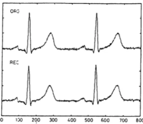
( s e c · ) T i m e ( s e c · )

Figure 3.12: The original and the reconstructed ECG leads, /,//,1^1 and V^2, for the case of raw data usage. CR{DCT) = 6.17, APRD = 6.19%.

CHAPTER 3. MULTICHANNEL ECG DATA COMPRESSION 36

V5

V5

V6

V6

I---1--- 1--- 1--- 1--- 1--- r~

0.00

0.80

1.60

2.40

T i m e ( s e c · ) I--- 1--- 1--- 1--- 1 I r ~

0.00

0.80

1.60

2.40

T i m e ( s e c · )

Figure 3.13: The original and the reconstructed leads, F3,V'4, F5 and V6 tor the raw data usage. CR{DCr) = 6.17, APRD = 6.19%.

II

_II

V1

V1

I---

1---1---0.00

0.80

T i m e 1--- 1--- 1--- r—

1.60

2.40

( s e c . ) I--- -

1---0.00

0.80

T i m e T--- T"

1.60

T---\—

2.40

( s e c · )

Figure 3.14: The original and the reconstructed leads, /, II, VI and V2 for the 30 Hz low pass filtered data usage. CR{DCT) = 8.69, APRD = 3.41%.