Impact of macroeconomic indicators on short selling: evidence from the Tokyo stock exchange

(1)

C H A P T E R 1 9

Impact of Macroeconomic Indicators on

Short Selling: Evidence from the Tokyo

Stock Exchange

M. Nihat Solakoglu and Mehmet Orhan

ABSTRACT

This study is an attempt to analyze the behavior of short selling due to changes in main macroeconomic indicators of output, interest rate (in terms of bond yields), and exchange rate, as well as the stock exchange index, namely the Nikkei 225. In addition, this chapter examines the existence of cointegration between short selling volume and the Nikkei 225 Index to inves-tigate the permanent relation between the two. We have intentionally used monthly Japanese data from November 2005 to October 2009 to encompass the global financial crisis and differenced the series to attain stationarity. Our Granger test of causality concluded a bidirectional relation between short selling and the Nikkei 225. We could not verify causality between short selling and gross domestic product, as well as the exchange rate, but there is causality from the exchange rate to short selling.

Handbook of Short Selling.DOI: 10.1016/B978-0-12-387724-6.00019-2

(2)

KEYWORDS

Augmented Dickey–Fuller test; Bond yield; Consumer price index; Exchange rate; Granger test; Gross domestic product; Interest rate; Macroeconomic indicators; Nikkei 225 Index; Output.

19.1 INTRODUCTION

Short selling has received a lot of attention in the last decade by academi-cians, regulators, and investors. While some academicians argue that short selling leads to higher market efficiency, others argue that short sellers are investors with private information that aim to profit at the expense of naïve investors. If the second view is correct, then we should also expect to observe higher volatility in the markets due to short selling. Given the vary-ing degrees of restrictions imposed on short sellvary-ing in major markets startvary-ing in 2008 due to the global crisis, we can assume that regulators prefer to accept the second view over the first. For instance, in 2008, a wave of restric-tions on short selling, some being temporary, was announced for more than 20 major markets.1 In particular, for Japan, short sales of all stocks were prohibited until March 2009 and naked short selling was prohibited. More-over, the threshold for disclosure obligation was set to 0.25% or more of outstanding stocks.2

Is there a strong relationship between short selling and abnormal returns? In other words, can short sellers predict a decline in share prices so that they can profit by short selling? Some studies’ findings indicate that traders cannot profit through short selling strategies. For instance, Figlewski and

Webb (1993)find no evidence between short selling and abnormal returns.

Similarly, Brent, Morse, and Stice (1990)and Woolridge and Dickinson

(1994)document no evidence between short selling and abnormal returns.

Using the TA100 index of the Tel Aviv Stock Exchange, Cohen (2010) suggests that short sellers cannot outperform the market and hence con-tribute to market efficiency in the long run. However,Asquith and Meulbroek

(1996) focus on firms with large short positions to examine whether short

sellers are able to profit. Their finding shows a strong and consistent rela-tionship between short positions and abnormal returns indicating the ability of firms with large short positions to profit. This should not be surprising, as firms with large short positions are expected to be more informed or 1_{Introduction of new regulations for short selling in the United States by the SEC in 2005, short-term}

ban of short selling in the United States in 2008, in the United Kingdom, and total ban in Australia can be used to show how regulators view short selling.

2_{For details, please see}_{http://www.fsa.go.jp/en/news/2008/20081027-2.html}_{page from Financial}

(3)

have access to private information. This finding is consistent withBoehmer,

Jones, and Zhang (2008)andBlau, Van Ness, and Van Ness (2010) as they

both find evidence that traders with larger short sales are more informed than traders with smaller short sales.Blau and associates (2010)also docu-ment that, with greater market efficiency, short sellers will have difficulty in predicting future negative returns correctly using NASDAQ and NYSE short selling data.3

For the Australian Stock Exchange,Aitken, Frino, McCorry, and Swan (1998) provide evidence that short sales result in bad news for the market.Christophe,

Ferri, and Angel (2004)andChristophe, Ferri, and Hsieh (2010)document

that the majority of short sellers are informed traders and are able to target stocks with overvalued prices or potential downgrades. Moreover,Christophe

and colleagues (2004)find some evidence of a higher level of short selling for

firms with a negative earnings announcement. TheChristophe and colleagues

(2010)study suggests a similar finding for analysts’ downgrade decisions. Both

findings imply that short sellers are informed traders.

Prior studies assume short sellers either as informed traders or uninformed hedgers/speculators.4For uninformed traders, there should not be a consis-tent and significant relationship between short selling and abnormal returns. If short sellers are informed traders, then they should be able to select over-priced stocks or use the same set of information as stock analysts to come up with the same downgrade decision. An alternative could be acquisition of private information of a stock that is not publicly available. For example, short sellers may receive tips from a brokerage firm for a potential down-grade of a stock and then utilize this information to profit. The findings of

Christophe and colleagues (2010)show some evidence that short sellers

receive some private information, whereasDiether, Lee, and Werner (2007) argue that the tipping hypothesis5is highly unlikely to occur as there are strict regulations levied on corporate insiders. This is true with approxi-mately 75% of short sellers being institutional investors in the United States (as implied byBoehmer & colleagues, 2008).

A third alternative is short sellers acting as voluntary market makers, as dis-cussed byDiether and colleagues (2007)andKo and Lim (2006). An exception to this alternative is short sellers in Japan. Approximately 10% of short sellers in Japan are exchange member firms, while the rest include customers such as foreigner investors, corporations, and individual investors, which consist of 3_{Specifically, they argue that NYSE is more efficient compared to NASDAQ and hence short selling is}

more predictive picking out stocks with a potential decline on NASDAQ than NYSE.

4_{Some informed traders will not participate actively in short selling due to legal or regulatory}

constraints (Christophe & colleagues, 2010).

5_{Prereleasing research to certain preferred investors before it is distributed widely.}

(4)

the majority. As a result, it can be argued that short sellers in Japan do not have private information and have no obligation to provide market liquidity.6 However,Ko and Lim (2006) document that a positive relationship exists between short interest and abnormal return; hence, even in the absence of market makers short sellers’ actions provide liquidity to the markets.

In this study, we intend to analyze short selling in Japan using selected macroeconomic indicators of output, interest rate, and exchange rate. As indi-cated byKo and Lim (2006), short sellers in Japan are mostly individual cus-tomers with no private information and hence we expect them to pay close attention to economic fundamentals as well as firm-related news. The sample we use includes monthly data of short selling volume from the Tokyo Stock Exchange and macroeconomic data including the Nikkei 225 Index for the period from November 1, 2005, to September 30, 2009. Our period of study is selected intentionally to encompass the global financial crisis.

After the introduction, the rest of the study is organized as follows:Section 19.2 reviews briefly the Japanese macroeconomic indicators.Section 19.3is retained to data and methodology, where we start with unit root tests of variables. Given that we are working with time series data, we examine the stationarity of all the series at the beginning of the period using the augmented Dickey–Fuller test. We then investigate the existence and direction of causality, with the so-called Granger causality test, and the cointegrating relation between short selling volume and the Nikkei 225 Index.

19.2 DATA AND BRIEF OVERVIEW OF JAPANESE

MACROECONOMIC INDICATORS

Monthly short selling figures come from the archives of the Tokyo Stock Exchange.7The data set is monthly and covers November 1, 2005, through September 30, 2009. All remaining macroeconomic data series are from Nikkei (www.Nikkei.com).

Figure 19.1 plots the real gross domestic product (GDP) index. The plot

reveals that the Japanese economy was in recession during our sample period. The last decade of the Japanese economy was associated with a low growth rate, failure in attaining full employment, and persistent deflation. Export-led growth, existing before 2007, came to a standstill in 2008. In addition, the recession intensified as a consequence of the global financial crisis with less expectation for constant growth in the coming years due to an added uncertainty in forecasts. The continued quantitative easing of the 6_{In that case, we should assume that the}_{“tipping hypothesis” does not hold in Japan.}

(5)

Real GDP index 13,600 13,400 13,200 13,000 12,800 12,600 12,400 12,200 2005-112006-12006-32006-5 2006-72006-92006-112007-12007-32007-52007-72007-92007-112008-12008-32008-52008-72008-92008-112009-12009-32009-52009-72009-9 2005-112006-12006-32006-52006-72006-92006-112007-12007-32007-52007-72007-92007-112008-12008-32008-52008-72008-92008-112009-12009-32009-52009-72009-9 2005-112006-12006-32006-52006-72006-92006-112007-12007-32007-52007-72007-92007-112008-12008-32008-52008-72008-92008-112009-12009-32009-52009-72009-9 6.0 5.0 4.0 3.0 2.0 1.0 0.0 160.00 140.00 120.00 100.00 80.00 60.00 40.00 20.00 0.00 Foreign trade Unemployment rate FIGURE 19.1

Main macroeconomic indicators in the Japanese economy.

(6)

U.S. dollar by the Federal Reserve is expected to increase the price of the Japanese yen in terms of the U.S. dollar. Hence, we should not expect improvement in the export growth rate and export-led growth for the Japanese economy. According to Figure 19.1, the real GDP index grew gradually from the end of 2005 to early 2008, right before the crisis impacted the Japanese economy, as evidenced by a decline in real GDP. This decline continued until mid-2009 and decreased the real GDP index to its lowest value since late 2005 or early 2006.

Although the Japanese economy grew slightly during the 2005–2008 period, the unemployment rate appears to have hovered around 4% until early 2008. The Japanese economy is far from full employment levels, and the unemployment rate has been reported greater than 5% in recent months. Due to the stimulus package aimed at small businesses and local govern-ments, more than $60 billion announced by the cabinet helped decrease the unemployment rate below the 5% level. As shown in Figure 19.1, Japanese trade had a slight positive trend until September 2008, and the decline started right after that, largely due to the tightening of global demand to Japanese commodities and services.

Figure 19.2 presents the behavior of the consumer price index (CPI),

exchange rate between Japanese yen and U.S. dollar, and 10-year govern-ment bond yield rate between 2005 and 2009. The CPI stayed within a tight band—between the levels of 99 and 103, except through a short period dur-ing the credit crisis, where the upper bound was actually at an index level of 101. This stability of the Japanese CPI had a record of a −2.5% inflation rate during the last 50 years. A negative inflation rate is undesirable for an economy as it will deteriorate corporate profits and will place pressure on wage rates. As documented byFigures 19.1 and 19.2, the Japanese economy appears to be in recession with periods of deflation as a result of weak demand. Finally, the Japanese yen starts appreciating against the U.S. dollar since mid-2007 and against the euro since late 2008, putting more pressure on Japanese exports. The large appreciation of the Japanese yen against the euro during 2008 was mainly caused by depreciation of the euro against the U.S. dollar. The quantitative easing programs by the Federal Reserve Bank will likely not improve exchange rates in favor of Japanese exports. The plot of the 10-year Japanese government bond yield rate implies that the real interest rate is approximately zero percentage point per year, indicating slug-gish growth in the Japanese economy. Consistent with the aforementioned indicators, the interest rate does not change significantly during the exam-ined period, and it was never reported more than 0.10% in 2010.

Figure 19.3 plots total volume of short selling volume and the Nikkei 225

(7)

CPI 103.0 102.0 101.0 100.0 99.0 98.0 97.0 2005-112006-12006-32006-5 2006-72006-92006-112007-12007-32007-52007-72007-92007-112008-12008-32008-52008-72008-92008-112009-12009-32009-52009-7 2009-9 2005-112006-12006-32006-52006-72006-92006-112007-12007-32007-52007-72007-92007-112008-12008-32008-52008-72008-92008-112009-12009-32009-52009-72009-9 2005-112006-12006-32006-52006-72006-92006-112007-12007-32007-52007-72007-92007-112008-12008-32008-52008-72008-92008-112009-12009-32009-52009-72009-9 180.00 160.00 140.00 120.00 100.00 80.00 40.00 20.00 60.00 0.00 2.500 2.000 1.500 1.000 0.500 0.000

10-year government bond yield rate Exchange rates

Yen/Dol Yen/euro

FIGURE 19.2

Consumer price index, exchange rate, and government bond yield.

(8)

Nikkei 225 Index being smoother. The high correlation coefficient of 0.76 between these two variables supports the visual finding as well. Both series display a decline in their levels at the start of the global financial crisis, con-sistent with the macroeconomic series. The decline in short selling volume after March 2008 is most likely influenced by the restrictions imposed on short selling in Japan and in the rest of the world during 2008.

If short sellers are informed traders, which is more likely for Japan as most short sellers are customers and not exchange member firms (Ko & Lim, 2006), they should follow macroeconomic series closely as well as firm-specific information to predict a decline in share prices. For our analysis, we consider the Nikkei 225 Index, the government bond yield rate, foreign exchange rates, and GDP as the relevant macro series.

2005-112006-12006-32006-52006-72006-92006-112007-12007-32007-52007-72007-92007-112008-12008-32008-52008-72008-92008-112009-12009-32009-52009-72009-9 16,000 14,000 12,000 10,000 8000 6000 4000 2000 0 Short selling 2005-112006-12006-32006-52006-72006-92006-112007-12007-32007-52007-72007-92007-112008-12008-32008-52008-72008-92008-112009-12009-32009-52009-72009-9 20000.0 18000.0 16000.0 14000.0 12000.0 8000.0 10000.0 6000.0 4000.0 2000.0 0.0 Nikkei 225 FIGURE 19.3

(9)

19.3 DATA AND METHODOLOGY

Monthly short selling values are obtained from the archives of the Tokyo Stock Exchange8from November 2005 to September 2009. All macroeco-nomic data and stock index series are obtained from the Nikkei Web page (www.Nikkei.com).

19.3.1 Granger Causality between Macroeconomic

Variables and Short Selling

We first check for the stationarity of the time series to avoid spurious regres-sion.Dickey and Fuller (1979)designed a model to check for the existence of a unit root and subsequently use an improved model called the “aug-mented Dickey–Fuller (ADF) test” (Dickey & Fuller, 1981).

We make use of the ADF test, which suggests the following model:

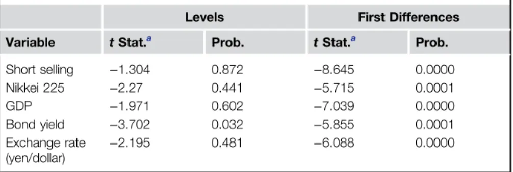
Δyt= α + βt + λyt−1+ δ1Δyt−1+ δ2Δyt−2+ … + δpΔyt−p+ εt (19.1) In this model,β is the coefficient of time to account for trend and p is the lag order of the autoregressive process. The test checks whetherλ = 0 or not, with the help of critical values, listed specifically for this test. We use E-Views soft-ware to execute the ADF test and report the results for both levels and first differences of the series inTable 19.1. According to the test results, all series, with the exception of“bond yields,” have unit roots and are not stationary at levels, but the first differences of all series are stationary. Test results, as shown inTable 19.1, show explicitly that the series under examination have changing mean and/or autocorrelation over time. Although it is not necessary to attain stationarity, we take the difference of the“bond yields,” as we would like to have all variables in differences.Table 19.1indicates that all variables are stationary at their first differences.

Table 19.1 Unit Root Test Results at Levels, HoClaims“No Unit Root”

Levels First Differences Variable t Stat.a Prob. t Stat.a Prob. Short selling −1.304 0.872 −8.645 0.0000 Nikkei 225 −2.27 0.441 −5.715 0.0001 GDP −1.971 0.602 −7.039 0.0000 Bond yield −3.702 0.032 −5.855 0.0001 Exchange rate (yen/dollar) −2.195 0.481 −6.088 0.0000 a

1, 5, and 10% critical values are −4.176, −3.513, and −3.187, respectively.

8_{http://www.tse.or.jp/english}_.

(10)

One approach in examining the relationship between interacting variables is to look at the causality among these variables. Granger (1969)designed a statistical test, called the “Granger causality test,” using a series of t tests and F tests to determine whether one time series is useful in predicting another time series. The Granger causality test does not necessarily address the cause-and-effect relation between variables as it may not indicate true causality.9We assume that xt and yt are two stationary series; to determine whether xtGranger causes yt, first ytis autoregressed on itself and the proper lag length is determined. In the next step the augmented autoregression of

yt= α0+

∑

i=1,:::,p

αiyt−i+

∑

j=1,:::,q

βjxt−j+ εt (19.2)

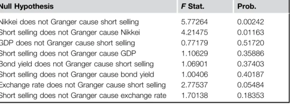
is estimated. The null hypothesis of “no Granger causality” is tested with a version of the F test, which checks whether all coefficients of xt−j, namelyβt−j, are equal to 0. If allβt−jare found to be equal to 0, then xt−jdoes not precede yt−j. Table 19.2presents results for the causality test. To perform the test, we focus on the short selling volume and the macroeconomic variables considered as part of the short sellers’ information set.

The null hypothesis of “no Granger causality” is rejected highly significantly for the relationship between the short selling volume and the Nikkei 225 Index with a p value of 0.242%. However, the causality test reveals causality from the short selling volume and the Nikkei 225 Index with a lower signif-icance level of 1.163%. Thus, test results document bidirectional causality of Granger type between the Nikkei 225 Index and the short selling volume. We find no indication of causality between short selling volume and GDP, and the same is true for the bond yield return.

Table 19.2 Granger Causality Test Results of Variables with First Differences

Null Hypothesis F Stat. Prob. Nikkei does not Granger cause short selling 5.77264 0.00242 Short selling does not Granger cause Nikkei 4.21475 0.01163 GDP does not Granger cause short selling 0.77179 0.51720 Short selling does not Granger cause GDP 1.10629 0.35886 Bond yield does not Granger cause short selling 1.06901 0.37403 Short selling does not Granger cause bond yield 1.00406 0.40187 Exchange rate does not Granger cause short selling 2.77537 0.05484 Short selling does not Granger cause exchange rate 1.70138 0.18353

9_{For example, if there is a third series that causes the first and second series to change, it is possible}

(11)

Although GDP is the most widely used indicator for the economic performance of a country, it does not appear as a variable that leads to short selling. Given the low levels of GDP growth rates in Japan and no big surprises for expected changes in the past for the Japanese economy, this should not be surprising. Finally, we find empirical evidence that documents causality from exchange rates and short selling volume.

19.3.2 Cointegration between Short Selling Volume and

the Nikkei 225 Index

Following Table 19.3results, we investigate the existence of a permanent relationship between short selling volume and the Nikkei 225 Index in this part of the study. Cointegration between variables is a convenient way to propose the long-run relationship between them. If there is a list of series, say Yt= ðY1t, Y2t,…, YntÞ, then this set of series is called “cointegrated” if coefficients exist,β = ðβ₁,β2,…, βnÞ, to satisfy β1Y1t+ β2Y2t+ … + βnYnte Ið0Þ, where Ið0Þ denotes stationarity of the series. If cointegration is proven for a series, then there is a long run equilibrium, and occasional deviations from the streamline will be removed to restore the equilibrium.

We look for a cointegration relationship between short selling volume and the Nikkei 225 Index with the assumption of a linear deterministic trend. Cointegration test results are reported inTable 19.3. Findings indicate that

Table 19.3 Cointegration between Short Selling Volume and Nikkei 225 Index, Test Results

Trace Test

Hypothesized Trace 5% 1% No. of CE(s) Eigenvalue Statistic Critical value Critical value None 0.165754 8.807615 15.41 20.04 At most 1 0.010191 0.471180 3.76 6.65

Maximum Eigenvalue Test

Hypothesized Maximum Eigen 5% 1% No. of CE(s) Eigenvalue Statistic Critical value Critical value None 0.165754 8.336435 14.07 18.63 At most 1 0.010191 0.471180 3.76 6.65

Normalized Cointegrating Coefficients (Standard Error in Parentheses) Nikkei Short sell

1.000000 −1.650126 (0.30444)

(12)

the null hypothesis of “at most 1 cointegration relation” is not rejected according to the values of both trace and maximum eigenvalue statistics. This implies that short selling volume and the Nikkei 225 Index have a per-manent, long run relationship for the Japanese economy during the investi-gation period. Table 19.3 displays normalized cointegration coefficients as well as standard errors in the bottom rows.

19.4 CONCLUSION

We examined Japanese financial markets with monthly data from November 2005 to October 2009 to document if a causality relation exists between short selling volume and macroeconomic variables, such as GDP, bond yield, and exchange rate, as well as the Nikkei 225 Index. Given the charac-teristics of Japanese short sellers, we expect a causal relationship between macroeconomic variables and short selling volume, which indicates that Japanese short sellers are informed traders. Based on this finding, we can also assume indirectly that the tipping hypothesis does not apply to Japanese short sellers. In addition, we also investigated the existence of coin-tegration between short selling volume and the Nikkei 225 Index to deter-mine whether a long run relationship exists between the two.

We found that the short selling volume, the Nikkei 225 Index, and the exchange rate have unit roots and are thus nonstationary; however, the bond yield rate is stationary. We achieved stationarity of the series at their first differences. Using the Granger causality test, we also showed bidirectional causality between short selling volume and the Nikkei 225 Index. However, there is no causality between short selling volume and GDP, as well as bond yield rate. However, our findings document that exchange rate Granger causes a short selling volume, but short selling volume does not Granger cause exchange rate. These findings indicate that the short sellers’ information set contains the Nikkei 225 Index and exchange rate movements, but not macro fundamentals. Our results also document the permanent long run relation-ship between short selling volume and the Nikkei 225 Index.

We documented a cointegration relationship between short selling volume and the Nikkei 225 Index. Further research in this direction may continue with construction of an error correction mechanism to explore the duration of the regression toward the mean over the long run in case of a shock to the economy.

Money managers dealing with the Japanese market should concentrate on the two findings of this study. First, short sellers are informed traders and their information set does not include private information. Second, the information set contains information mostly from stock and currency

(13)

markets and does not seem to be influenced by economic fundamentals. Hence, the prediction of stock price declines, instead of relying on tips, using the aforementioned information set with firm level information, may be a profitable strategy by short selling in the Japanese market.

DATA APPENDIX

Real GDP Index Unemp. Rate (%) Trade CPI Nikkei 225 Yen/$ Yen/€ Gov. Bond Yield Short Selling Total 2005-11 12,711 4.5 112.33 100.0 14368.1 118.41 139.54 1.445 8795 2005-12 12,825 4.4 117.66 100.0 15650.8 118.64 140.68 1.470 8830 2006-1 12,877 4.4 104.02 99.7 16085.5 115.45 139.99 1.560 9232 2006-2 12,865 4.1 107.89 99.5 16187.6 117.89 140.77 1.585 10,399 2006-3 13,006 4.1 126.89 99.9 16311.5 117.31 140.98 1.770 8902 2006-4 12,928 4.1 116.47 100.0 17233.0 117.11 143.56 1.920 8889 2006-5 12,984 4.1 110.51 100.2 16322.2 111.51 142.54 1.830 9611 2006-6 12,975 4.2 117.42 100.2 14990.3 114.53 145.14 1.920 10,386 2006-7 12,943 4.1 117.90 100.1 15147.6 115.67 146.72 1.915 9103 2006-8 12,958 4.1 120.89 100.3 15786.8 115.88 148.47 1.620 9244 2006-9 12,996 4.1 126.50 100.4 15934.1 117.01 149.11 1.670 8583 2006-10 13,017 4.1 125.82 100.4 16519.4 118.66 149.66 1.720 9722 2006-11 13,093 4.0 123.51 100.2 16101.1 117.35 151.13 1.645 9578 2006-12 13,072 4.0 128.09 100.1 16790.2 117.30 154.92 1.675 8716 2007-1 13,067 4.0 119.04 99.7 17286.3 120.58 156.56 1.695 9149 2007-2 13,149 4.0 118.71 99.4 17741.2 120.45 157.60 1.630 11,242 2007-3 13,053 4.0 134.23 99.6 17128.4 117.28 155.29 1.650 12,381 2007-4 13,187 3.8 123.64 99.9 17469.8 118.83 160.36 1.615 10,552 2007-5 13,211 3.8 127.40 100.1 17595.1 120.73 163.19 1.745 12,077 2007-6 13,185 3.7 133.26 100.1 18001.4 122.62 164.48 1.865 11,360 2007-7 13,175 3.6 134.44 100.0 17974.8 121.59 166.68 1.790 10,961 2007-8 13,273 3.7 133.26 100.2 16461.0 116.72 158.98 1.600 14,365 2007-9 13,357 4.0 129.02 100.3 16235.4 115.02 159.64 1.675 9298 2007-10 13,310 4.0 140.14 100.5 16903.4 115.74 164.74 1.600 11,399 2007-11 13,344 3.8 137.53 100.6 15543.8 111.21 163.28 1.460 11,920 2007-12 13,436 3.8 140.01 100.9 15545.1 112.34 163.50 1.500 9076 2008-1 13,452 3.9 129.23 100.5 13731.3 107.66 158.14 1.440 11,651 2008-2 13,264 4.0 130.12 100.4 13547.8 107.16 158.18 1.355 10,868 2008-3 13,300 3.8 142.67 100.8 12602.9 100.79 156.28 1.275 10,474 2008-4 13,303 3.9 133.20 100.8 13355.8 102.49 161.53 1.575 10,094 2008-5 13,325 4.0 132.73 101.6 13995.3 104.14 162.05 1.740 10,277 2008-6 13,447 4.0 142.00 102.0 14084.6 106.90 166.23 1.610 10,537 2008-7 13,324 4.0 151.67 102.4 13168.9 106.81 168.35 1.530 10,856 Continued... 19.4 Conclusion 299

(14)

Real GDP Index

Unemp. Rate

(%) _Trade _CPI Nikkei₂₂₅ _Yen/$ _Yen/_€

Gov. Bond Yield Short Selling Total 2008-8 13,213 4.1 144.17 102.6 12989.4 109.28 163.75 1.405 9196 2008-9 13,132 4.0 146.32 102.6 12123.5 106.75 153.25 1.480 9270 2008-10 13,072 3.8 139.05 102.4 9117.0 100.33 133.49 1.480 9313 2008-11 13,080 4.0 108.75 101.6 8531.5 96.81 123.25 1.395 6432 2008-12 12,830 4.4 99.83 101.1 8463.6 91.28 122.79 1.165 5970 2009-1 12,855 4.2 79.24 100.5 8331.5 90.41 119.68 1.270 5706 2009-2 12,831 4.4 69.88 100.4 7694.8 92.50 118.33 1.270 6106 2009-3 12,816 4.8 83.73 100.7 7764.6 97.87 127.44 1.340 6597 2009-4 12,823 5.0 83.40 100.7 8768.0 99.00 130.50 1.430 6522 2009-5 12,846 5.1 77.59 100.5 9304.4 96.30 131.92 1.480 5714 2009-6 12,764 5.3 87.02 100.3 9810.3 96.52 135.46 1.350 7014 2009-7 12,805 5.6 93.20 100.1 9691.1 94.50 133.00 1.415 6590 2009-8 12,868 5.4 88.54 100.1 10430.4 94.84 135.31 1.305 5878 2009-9 12,912 5.3 97.01 100.2 10302.9 91.49 132.80 1.295 6429 2009-10 13,063 5.2 98.17 100.1 10066.2 90.29 133.87 1.405 5505

REFERENCES

Aitken, M., Frino, A., McCorry, M. S., & Swan, P. L. (1998). Short sales are almost instanta-neously bad news: Evidence from the Australian Stock Exchange. Journal of Finance, LIII(6), 2205_–2223.

Asquith, P., & Moelbroek, L. (1996). An empirical investigation of short interest. Working Paper, Harvard University, Cambridge.

Blau, B. M., Van Ness, B. F., & Van Ness, R. A. (2010). Information in short selling: Comparing NASDAQ and the NYSE. Review of Financial Economics, doi:10.1016/j.rfe.2010.09.002. Boehmer, E., Jones, C. M., & Zhang, X. (2008). Which shorts are informed? Journal of Finance,

63, 491_–527.

Brent, A., Morse, D., & Stice, E. K. (1990). Short interest: Explanations and tests. Journal of Finan-cial and Quantitative Analysis, 25, 273–289.

Christophe, S. E., Ferri, M. G., & Angel, J. J. (2004). Short-selling prior to earnings announce-ments. The Journal of Finance, LIX(4), 1845–1875.

Christophe, S. E., Ferri, M. G., & Hsieh, J. (2010). Informed trading before analyst downgrades: Evidence from short sellers. Journal of Financial Economics, 95, 85_–106.

Cohen, G. (2010). Do short sellers outperform the market? Applied Economics Letters, 17, 1319–1322. Dickey, D. A., & Fuller, W. A. (1979). Distribution of the estimators for autoregressive time

series with a unit root. JASA, 74, 427_–431.

Dickey, D. A., & Fuller, W. A. (1981). Likelihood ratio statistics for autoregressive time series with a unit root. Econometrica, 49, 1057–1072.

(15)

Diether, K., Lee, K.-H., Werner, I. (2007). Can short-sellers predict returns? Daily evidence. Fisher College of Business, Working Paper Series, Ohio State University.

Figlewski, S., & Webb, G. P. (1993). Options, short sales, and market completeness. Journal of Finance, 48, 761_–777.

Granger, C. W. J. (1969). Investigating causal relations by econometric models and cross-spectral methods. Econometrica, 37(3), 424–438.

Ko, K., & Lim, T. (2006). Short selling and stock prices with regime switching in the absence of market makers: The case of Japan. Japan and the World Economy, 18, 528–544.

Woolridge, J. R., & Dickinson, A. (1994). Short selling and common stock prices. Financial Analysts Journal, 50, 20_–28.

Impact of macroeconomic indicators on short selling: evidence from the Tokyo stock exchange

C H A P T E R 1 9