Fast direct volume rendering of unstructured grids

(1)

FAST DlilECT VÖLUMB RENDEIING

OF UNSTP.ÜCTUS.ED GRIDS

(2)

FAST DIRECT X’OLUME RENDERING

OF UNSTRUCTURED GRIDS

A THESIS

SUBMITTED TO THE DEPARTMENT OF COMPUTER ENGINEERING AND INFORMATION SCIENCE AND THE INSTITUTE OF ENGINEERING AND SCIENCE

OF BILKENT UNI\’ERSITY

IN PARTIAL FULFILLMENT OF THE REQUIREMENTS FOR THE DEGREE OF

MASTER OF SCIENCE

H-c^U

By

Hakan Berk

September. 1997

(3)

T

-

6 4

(4)

I certify that 1 have read this thesis and that in my opin ion it is fully adequate, in scope and in quality, as a thesis for the degree of Master of Science.

Assoc. Prof. Cevdey.Avkanat(Principal .Advisor

I certify that I have read this thesis and that in my opin ion it is fully adequate, in scope and in quality, as a thesis for the degree of Master of Science.

-Prof. Bülent Özgüç

I certify that I have read this thesis and that in my opin ion it is fully adequate, in scope and in quality, as a thesis for the degree of .Master of Science.

-7 \ i I < ·'. /”

1

^

.... —_

.Asst. |*rof. I'^ ir Güdükbay

.Approved for the Institute of Engineering and Science:

Prof. Dr. .Mehmet

(5)

ni

ABSTRACT

FAST DIRECT VOLUME RENDERING OF UNSTRUCTURED GRIDS

Hakan Berk

M.S. in Computer Engineering and Information Science Supervisor; Assoc. Prof. Cevdet .Aykanat

September. 1997

Scientific Computing has become more and more important with the evolv ing technology. The vast amount of data that the scientific computing applica tions produce need new ways to be processed and be interpreted by scientists. The large amount of data makes it very difficult for scientists to extract useful information from the data, and interpret it to reach a useful conclusion. Thus, visualization of such numerical data as an image, which is named as Scieinific

M sualization, is an indispensable tool for researchers, \ohime Rendering is a very important branch of Scientific Visualization and makes it possible for scientists to visualize the 3-dimensional (3D) volumetric datasets.

\blume Rendering algorithms can be classified into two categories; Indirect and Direct methods. Indirect methods are faster, but direct methods aie m()ie flexible, and accurate. Direct methods can be classified into three catc*gorie--;

im age-space (ray-casting), object-space (projection) and hybrid. The efficiencx of a direct volume rendering (DVR) algorithm is strongly related to the way that it solves the underlying point location and view sort problems. .Although these problems are almost trivial ones to solve in structured grids, they be come more complex ones to deal with for unstructured grids. Researchers ha\ e tried to speed up the volume rendering of unstructured grids by using spe cial graphics hardware, and parallel architectures, but the need for software solutions to these problems will always exist. This thesis is involved in solv ing those problems in unstructured grids via software methods. It investigates three distinct categories, namely im age-space methods, object-space methods and hybrid methods for fast direct volume rendering of unstructured grids.

(6)

IV

The main objective of the thesis is to identify the relative superiorities and inferiorities of the algorithms in these three categories. .A survey of e.xisting methods is enriched by a discussion of their merits and shortcomings. Three new and fast algorithms to overcome the e.xisting inefficiencies are proposed, and one existing algorithm is investigated in detail for a better comparison. .All of the proposed algorithms are aimed at producing correct, high qualii\· images. Two of the proposed algorithms are pure ray-casting based solutions that support earJv ray termination and can handle cyclic grids. The relati\e performances of the proposed algorithms are experimented on a wide range of benchmark grids in a common framework for software methods and they are found to be faster than the existing best DVR algorithms.

Key u'ords: Volume Rendering, Direct Volume Rendering (D\ R). I nstruc- tured Grid, \ olume Visualization. Ray Casting.

(7)

IV

ÖZET

DÜZENSİZ IZGARALARIN HIZLI DİREK HACİM GÖRÜNTÜLENMESİ

Hakan Berk. Bilgisayar ve Enformatik Mühendisliği. Yüksek Lisans Tez Y öneticisi: Doç. Dr. Cevdet Aykanat

Evlül. 1997

Bilimsel Hesaplama her geçen gün gelişen teknoloji ile daha da önem kazan maktadır. Bilimsel uygulamalar tarafından üretilen çok miktardaki verilerin bilimadamlannca işlenmesi ve daha kolay anlaşılabilmesi için yeni yöntemlere ihtiyaç duyulmaktadır. Üretilen verilerin yüksek miktarda olmasından dolayı bilimadamlarının bu verilerden anlamlı ve işe yarar bilgileri çıkarmaları zor laşmaktadır. Bu yüzden bu sayısal verilerin görüntülenmesi bilimadamları için vazgeçilemez bir araçtır, ve bilgisayar grafiklerinin bu konuyla uğraşan dalına da BHiınsel Görüntüleme adı verilir. .Ymaci 3-boyutlu hacimsel veri lerin görüntülenmesi olan Hacim Görüntüleme ise Bilimsel Görüntüleme'nin en önemli alt dallarından birisidir.

Hacim Görüntüleme yöntemleri iki sınıfa ayınlabilir; Dolayh ve D irek. Dolaylı yöntemler daha hızlıdır, fakat Direk yöntemler daha esnektir ve daha doğru sonuçlar verirler. Direk hacim görüntüleme yöntemleri de kendi içinde üçe ayrılırlar: ekran-uzayı (ışm izlem e), cisim-uzayı ve каппа yöntemler. Direk Hacim Görüntüleme (DHG) yöntemlerinin verimliliği daha çok nokta-yeri tespiti ve görüntü-sıralama problemlerini ne şekilde çözdüğüne bağlıdır. Bu problemlerin çözümü düzenli ızgaralarda basit olmasına rağmen.

düzensiz ızgaralarda daha zordur. .Araştırmacılar düzensiz ızgaraların hacim görüntülenmesini özel grafik donanımı, yada paralel mimariler kullanarak hız landırmaya çalışmaktadırlar, ama bu alanda yazılım çözümlerine her zaman ihtiyaç duyulacaktır. Bu tez düzensiz ızgaraların hacim görüntüleıırnesindeki problemlerin yazılım yöntemleri ile çözülmesi üzerinedir. Düzensiz ızgaraların hacim görüntülenmesi için olan üç ayrı kategorideki yöntemleri inceler. Tezin en önemli amaçlarından birisi değişik kategorilerdeki yöntemlerin avantaj ve dezavantajlarını saptamaktır. Bu konudaki önemli yöntemlerin tartışması.

(8)

bunların dezavantajlarının ve avantajlarının belirtilmesi ile zenginleştirilmeye çalışılmıştır. Bu problemleri çözmeye yönelik üç yeni ve hızlı yöntem geliştirilmiş ve daha iyi bir karşılaştırma için olan bir yöntem detaylı bir şekilde incelenmiştir. Tezde öne sürülen tüm yöntemler doğru ve yüksek kalite resim üretmeyi amaç edinmişlerdir. Bunlardan iki tanesi tamamen ışın-izleme üzerine geliştirilmiş yöntemler olup, erken ışın sonJanınasını desteklemekte ve döngüce] ızgaraları görüntüleyebilmektedirler. Bu yöntemlerin göreceli performansları geniş bir veri kümesi üzerinde deneysel olarak ölçülmüş ve olan en i\ i DH(i vöntemlerinden daha hızlı oldukları sonucuna varılmıştır.

Anahtar K d iım k r. Hacim Görüntüleme. Direk Hacim Görüntüleme. Düzensiz Izgara, Işın izleme.

(9)

VI

ACKNOWLEDGMENTS

I wish to express my deepest gratitude and thanks to Assoc. Prof. Cevdet Aykanat and Prof. Dr. Bülent Ozgüç for their supervision, encouragement, and invaluable advice throughout the development of this thesis.

I would like to thank Asst. Prof. I ğur Gûdükbay for reading my thesis, and his invaluable comments, suggestions and remarks.

I wish to extend my sincere thanks to all of my friends for their support during the development of the thesis. I would like to thank Ferit Fındık for his corporation on the codes written for the thesis work.

Finally. I would like to express my endless thanks to my family and Gave Tiizemen for their endless support and patience.

(10)

List of Figures

2.1 Types of grids encountered in volume rendering...

1

]

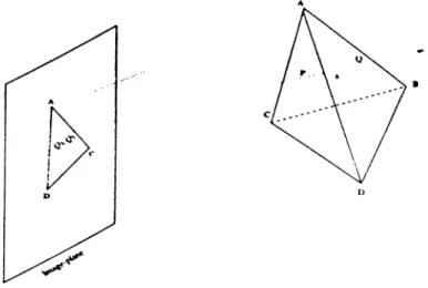
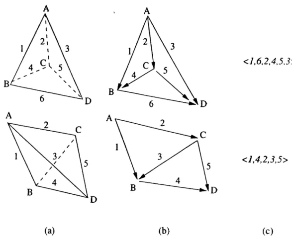
3.1 Shooting of a ray from image-plane, and following it in the vol ume using Koyamada's a lg o rith m ... 3S 3.2 (a) Two sample cells projected onto the screen with edge num

bering (Note that only back-face edges are numbered), (b) The corresponding directed graphs where depth-first search is per formed starting from the topmost vertex .4. (c) The correct back-face edge orderings... 3.3 A sample case of following a ray in SBRC algorithm, (a) R ayl

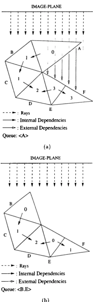
hits the Cell, and activates it. (b) Rayl reads the exit values from the span-buffer and continues in the volume, (c) Ray2 hits the Cell, and directly reads the values from the span-buffer. 3.4 .4 sample case from the rendering phase of .MC algorithm. The

numbers inside the cells show their current InDegrees (a) Queue is initialized with celL4. (b) .4fter cell A is processed, its depen dents B and E . are placed in the Queue...

4o

IS

4.1 Rendered images of the volumetric data sets used in performance analvsis... GG

(13)

LIST OF FIGURES

4.2 V'ariation of relative performances of the proposed algorithms with respect to Koyamada's algorithm with increasing resolution for (a) Blunt Fin. (b) Combustion Chamber, (c) Oxygen Post and (d) Delta Wing... 81

(14)

List of Tables

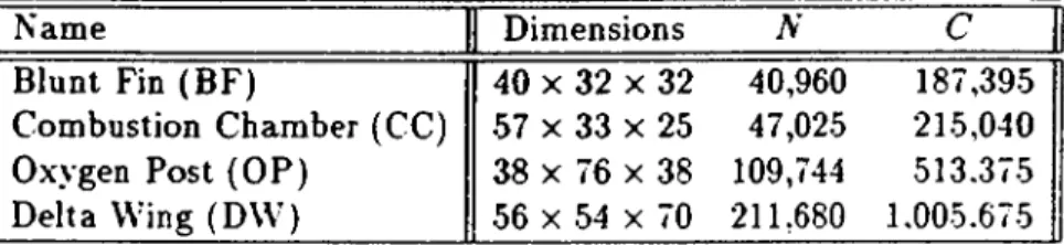
4.1 List of datasets used for testing. Dimensions are the original NAS.A Plot3D sizes. N and C represent the actual sizes used by the algorithms...

6

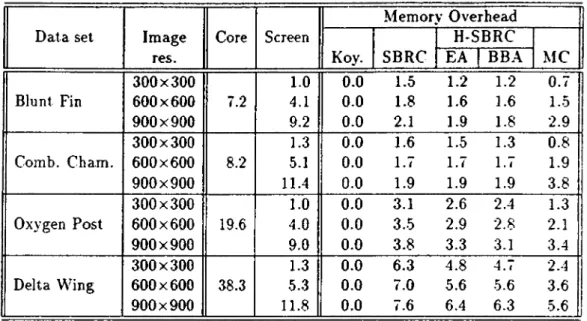
o 4.2 Memory consumptions of the algorithms in M Bytes...

68

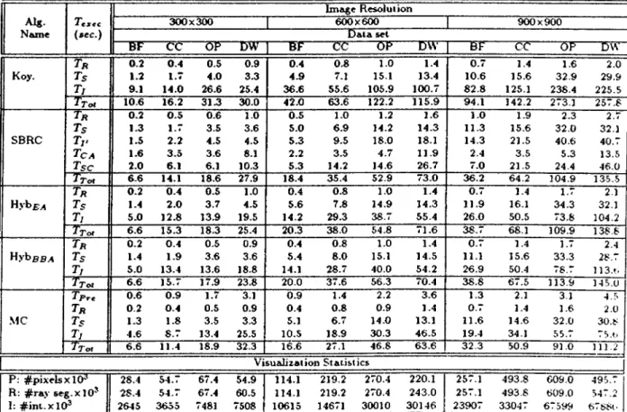
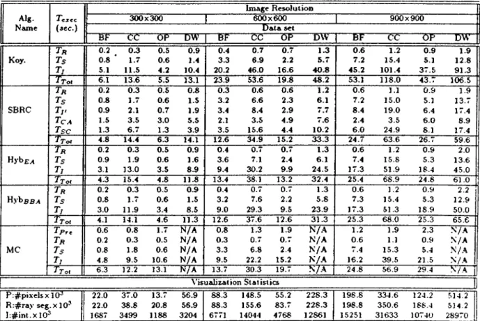
4.3 Execution-time dissection and visualization statistics of algo

rithms for view Vj. 76

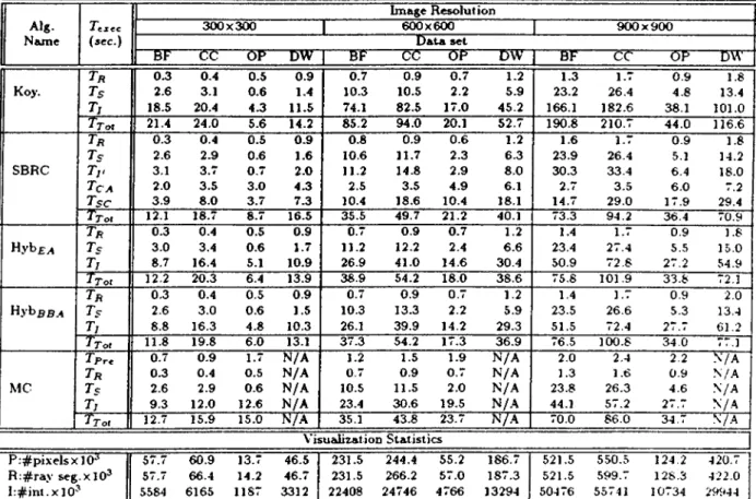
4.4 Execution-time dissection and visualization statistics of algo

rithms for view I

2

. 77

4.5 Execution-time dissection and visualization statistics of algo rithms for view I

3

... 78 4.6 Execution-time dissection and visualization statistics of algo

rithms for view I

4

. 79

4.7 Execution times of algorithms normalized with respect to those

of Koyamada's (for standard view I 'l). 79

4.8 Execution times of the proposed algorithms normalized with re spect to those of Koyamada's (averages of four views). X’alues with ‘ are averages of views I j and V

4

because of the cyclic meshes obtained in other views. V

2

and I

3

... 80

(15)

LIST OF TABLES XJ)

4.9 Performance comparison of presented algorithms with Lazy Sweep Ray-Casting (LSRC) algorithm for standard view I j . LSRC (Sun) values represent the run-time estimates of LSRC on Sun Ultra Enterprise 4000 system computed using specfp95 ratio of the Sun system to the SGI Power Challenge RlOOOO obtained from http://w w w .specben ch.org/osg/cpu95/resuIts/cfp95.htm l. . SO

0.1

Quality measure classification of software DVR methods for un structured grids... 85

(16)

Chapter 1 Introduction

The contribution of this thesis is primarily in Volume Rendering, \olunie Rendering has become one of the most important sub fields of Scientific \’isu-

alization. The main focus of this thesis is on fast direct volume rendering of unstructured grids.

Scientific \’isualization is a developing field of research. .As scientific ap plications become more comple.x. the methods to process data and interpret acquired results need to improve in parallel. At this point. Scientific \'isualization algorithms are utilized for detailed interpretation of those comple.x datasets to reach useful conclusions. Research in scientific visualization en compasses methods that act like a filter to transfer raw data into various kinds of representations where it is easier for human perception to interpret. This transformation usually occurs as mapping numerical data to sounds, images, etc. Therefore, scientific visualization can help the human mind process enor mous amount of data that normally would be beyond our capacity to deal with.

Scientific visualization tries to establish a general set of principles for \ isu- ally representing comple.x data structures. The most primitive scientific visu alization techniques include tables, different charts (e.g. bar. pie), and point plots. These are mainly useful for simple representation of functions of the

(17)

kind f{x ). Then comes the contours and images which help a lot in under standing functions of the kind f{ x ,y ) . These techniques are largely used in weather forecasting, and geography. So far. the techniques presented are suit able for use with scalar data, so none of them are able to represent a dataset where both magnitude and direction are of vital importance. In such cases, a vector representation will be inevitable. .Although, vectors are thought as tools to visualize multiple components of quantities like velocity and magnetic fields, they are also useful for interpretation of multidimensional gradients of scalar functions. .As the new parameters added, the existing methods become useless in representing the original dataset in the appropriate way that will be best to capture for human perception. For instance, none of the methods mentioned above are suitable for understanding the heat distribution on a wing of an aeroplane, or representing the data acquired by a M agnetic R esonance

(MR) scan device. The reason is that none of the above methods are suitable for the representation of 3 dimensional spatial data. The sub field of scientific visualization the main concern of which is to visualize 3 dimensional spatial data.sets is called Volume Rendering (\olume Visualization) [

1

. 2].

Volume rendering seeks methods to generate a meaningful image of volu metric data. The main goal is to produce a graphical representation of the volumetric data such that the scientist or engineer can interpret this complex dataset. Therefore, it must, somehow, be able to map various properties of the volumetric data in an intuitive and consistent way. More formally, volume rendering deals with the visualization of data sets that consists of large amount of numerical data values associated with points in 3 dimensional space.

CHAPTER 1. ISTRODVCTION

2

Three dimensional datasets are usually given as a set of points defined on 3 dimensional Cartesian space where each data point represents a scalar, vector, etc. value about an entity like a bone, tissue, or plane. These data points are called sampling points as they represent sample results about the property of the entity to be visualized. For instance, in medical imaging they can represent the density, whereas in the simulation of an aeroplane wing they may represent heat. The spatial topology of the distribution of the sample points in 3 dimen sional space is of vital importance in the visualization process. The major distinction that categorizes the grids that are formed of sampling points is the

(18)

regularity/irregularity of the structure. If the samples are distributed over a grid with equal or variable spacing where an implicit connectivity between the grid points exists, then it is called a structured grid. In this case, the sample points can be supplied as a simple

3

D computational virtual array where each neighbor relation in this array corresponds to the same neighbor relation in the

3

D Cartesian space. This sort of topology is common to medical imaging ap plications such as Com puter Tomography (CT) or Magnetic Resonance (MR). The grids that are in the form of the other type of topology are called unstruc tured grids. .As the name implies, there does not exist an implicit structure in the distribution so the connectivity relation must be supplied explicitly. These types of grids are common in Com putational Fluid Dynamics (CFD). Finite

Volume Analysis (FVA), and Finite Element Methods (FEM).

Usually, volume data is represented by

3

D voxels (Volume Elem ents) that constitute the atomic pieces of the overall data structure in the context of domain discretization. The shapes of the voxels are variant. The vertices of those voxels are the sample points discussed above. Therefore, there is a strong relation between the distribution of sample points, and the shapes of the voxels. The most common voxel shape in structured grids is a hexahedral that consists of

8

vertices. In unstructured grids, tetrahedral, and hexahedral voxel shapes are quite popular. The information about the attribute of the entity to be visualized is either stored in those voxels or in the sample points. This difference in the data is also reflected to visualization methods. .\ote that some authors use cell and voxel interchangeably, but in this work cell will l,)e used to avoid confusion. .Also throughout this thesis, the data model will l)e based on the assumption that the data values are stored at the sample points instead of the cells.

CHAPTER 1. INTRODUCTION

3

Volumetric datasets are rendered by finding the contributions of sample points to the pixels on the image plane. These contributions are determined via processing of the cells. The data values in the sample points are somehow mapped to color and opacity values via an optical model', and then those color, and opacity values are composited in the appropriate order to produce a meaningful image.

(19)

CHAPTER 1. ISTR O D VCTIO S

There are two major categories of volume rendering methods: Indirect (Sur

face based) and Direct m ethods. The methods that fall into the former categor\- try to track, and extract intermediate geometrical representation of the data, and render those surfaces via conventional surface rendering methods. Di rect methods render the data without generating an intermediate representa tion. Indirect methods are potentially faster, and are more suitable for medical imaging, and biological applications where the visualization of surfaces inside a volume makes sense (e.g. visualization o f tissues to identify a tumor). Di rect methods are slow due to massive computations performed, but give more accurate renderings. .As the direct methods do not rely on the extraction of surfaces, they are more general, and flexible. In one of the famous classifica tions of direct methods, they are classified into three categories: im age-space

(ray-casting), object-space (projection) and hybrid.

In general, volume rendering methods consist of two main phases. These are resampling and composition phases. In resampling phase, new samples are interpolated by using the original sample points. In composition phase, those new samples generated are mapped to color, and opacity values, and those color and opacity values are composited. In direct methods, resampling phase must be repeated for any change in the viewing parameters, but in indirect methods, once the isosurfaces are extracted, it should only be repeated if visualization parameters other than viewing parameters change. This is one of the reasons why indirect methods are faster than direct methods. During the resampling phase, the rendering method should somehow locate the new sample point in the cell domain, because the vertices of that cell, in which the new sample is being generated, will be used in the interpolation for the new sample. This problem is known as point location problem. In the composition phase, the color, and opacity values must be composited to determine the contribution of the data on a pixel. The composition operation is associative, but not commutative, therefore those color and opacity values should be composited in a predetermined (front-to-back or back-to-front) order. The determination of the correct composition order is known as view sort problem. These two problems are almost trivial ones to solve in structured grids, but the way that a volume rendering algorithm handles them is a crucial issue that strongly affects the performance of the rendering process for unstructured grids. The lack of

(20)

implicit connectivity between cells and the irregularity of the distribution of the sample points in the unstructured grids are the major factors that produce this difference.

Although volume rendering algorithms have become practical to use. there are still some problems to overcome. The most important of these problems is the speed of the rendering algorithms. Especially rendering of unstructured grids, which is the major concern of this thesis, is still far from interactive response times. The slowness of the volume rendering process create the lack of interactivity which in turn prevents it from being widely used. Therefore, indirect methods have become very popular in spite of the fact that they gi\e approximate and sometimes inaccurate images. Their interactive speed pre pared a platform for their widespread use. Then scientists began to use indirect methods for interactivity and experimentation, and rely on direct methods for accurate renderings. This is one of the major reasons why there is a need for faster direct volume rendering algorithms. In addition, it is very important for scientists to be able to change the simulation parameters so that the simulation is steered in the correct direction. Interactive visualization techniques could help the scientists experiment with the parameters to select the useful ones.

One of the attempts to speed up the visualization process is to rely on special graphics hardware, while some other researchers try to develop parallel algorithms. But nevertheless, the need for a software solution for fast rendering of unstructured grids will always exist. Therefore the main concern of this thesis will be on fast rendering of unstructured grids via software solutions.

1.1 Contribution of the Thesis

.As discussed in the previous sections, there is a need for fast volume rendering algorithms of unstructured grids on a software basis. This thesis investigates three distinct categories, namely image-space methods, object-space methods and hybrid methods for fast direct volume rendering of unstructured grids. The main objective of the thesis is to identify the relative superiorities and inferiorities of the algorithms in these three categories. .At least one algorithm

(21)

from each category is implemented and experimented in a common framework for software methods.

Koyamada’s algorithm [

4

]. being one of the outstanding algorithms of image- space methods, has been selected as the representative of image-space ap proaches in this framework.

new object-space method called Melting Cells (MC) algorithm, which differs from existing methods in its capability of producing high quality im ages and the sorting schema based on exploiting both image and object-space coherencies, is proposed.

Existing hybrid methods suffer from inability to support early ray termina tion and performing redundant computations especially in low resolutions as the portion of data contributing to the image is relatively small. .A new hy brid method, called Span-Buffer Ray-Casting (SBRC) algorithm is proposed to overcome all these deficiencies of the existing methods by changing the compu tational traversal order from object-then-image to image-then-object without comprimising full utilization of both image and object space coherencies ex ploited by Koyamada's and MC algorithm.

A fourth algorithm, namely Hybrid-SBRC (H-SBRC). stemmed from the idea of refining image-space and hybrid methods to extract the best features of each, is developed by blending Koyamada's and SBRC approaches. It exploits the computational traversal order proposed by SBRC algorithm to process small cells, where the overhead of using image-space coherency does not afford the gains expected, in a more cost effective way by employing a ray-casting schema which ignores image-space coherency, but still performs better. Two heuristics, namely E.xact .Area (E.A) and Bounding Box .Area (BB.A) approxi mation. have been proposed which are used in determining the cell-processing schema to be employed.

.Another contribution of the thesis is the proposal of optimization schemes to avoid the potential memory overheads without comprimising the run-time efficiency of the proposed algorithms.

(22)

versions of curvilinear NASA data sets widely used for benchmarking render ing algorithms. The relative performances of the algorithms are evaluated by the visualization of each of these data sets using four distinct views for three different resolutions for a better average case analysis.

The respective performances of the presented algorithms are compared with one of state-of-the-art algorithms called Lazy Sweep Ray-Casting (LSRC) [5] algorithm which is a hybrid approach and is reported to be two orders of magnitude faster than e.xisting software methods. Considering the run-time estimates of LSRC algorithm on our benchmark machine, MC algorithm is found to be

1.8

to 2.4. SBRC and H-SBRC algorithms are found to be 1.5 to

3.2

times faster than LSRC algorithm on the overall average. Restricted reported results of LSRC aJgorithm reveals that it scales slightly better than SBRC and H-SBRC algorithms, on the other contrary SBRC and H-SBRC algorithms scale much better than LSRC algorithm with increasing data set size.

7 1.2 Organization of the Thesis

The rest of the thesis is organized as follows.

In Chapter 2. an overview of volume rendering is presented. It ser\es as a kind of literature survev that describes the terminologv. and existing volume rendering methods. The main focus in this chapter will be on the pre^■iou^ work done for direct volume rendering of unstructured grids.

In Chapter 3, four algorithms that are the main concern of this thesis are introduced. The first algorithm is an e.xisting practical algorithm, called

Koyam ada's algorithm. Following that, three new algorithms proposed are explained, and discussed in detail.

In Chapter 4. the test data and experimental results obtained from the four algorithms discussed in this thesis are presented.

(23)

Finally, in Chapter 5, the results of the work done are discussed as conclu sion.

(24)

Chapter 2 Volume Rendering: An

Overview

"Visualization is a m ethod o f computing. It transforms the sym bolic into the geometric, enabling the researchers to observe their simulations and com pu tations. Visualization offers a m ethod for seeing the unseen. It enriches the process o f scientific discovery and fosters profound and unexpected insights. In many fields it is already revolutionizing the the scientists do science."

B. McCormick, T. DeFanti. and M. Brown. 1987. [

6

]

Scientific Computing has become more and more important with the evolv ing technology. The vast amount of data produced by the scientific computing applications need new ways to be processed and be interpreted by scientists. Ihis need emerged a new field in computer graphics which is called Scientific

Visualization. Scientific \'isualization covers a broad area from M edical Im ag

ing to Com putational Fluid Dynamics (CFD) simulations, and from weather forecasting to G eographical Information Systems (GIS). \oIume Rendering is a very important branch of Scientific Visualization.

(25)

CHAPTER 2. VOLUME RENDERIXG: AN OVERVIEW

10 2.1 Volume Rendering

Volume Rendering is a technique to visualize

3

-dimensional (3D) volumetric data that is in the form of a grid superimposed on a volume. The nodes of this grid contain the scalar values that represent the physical entity or the physical environment. For example, in medical imaging, magnetic resonance imaging (MRI) or positron emission tomography (PET) techniques are used to scan a specific part of the human body. The output of these techniques are in fact large amounts of numerical data in the form of a volumetric dataset, which when visualized in an abrupt way. will let the doctors see the different properties of tissues in that part of the body. In aerospace research, the scientists may want to visualize the heat distribution on a space shuttle, while in CFD simulations they will concentrate on visualization of vortices that are formed during the flow. The large amount of data makes it very difficult for scientists to extract useful information from the data, and interpret it to reach a useful conclusion. Thus, visualization of such numerical data as an image is an indispensable tool for researchers. Volume rendering makes it possible for scientists to visualize those volumetric data sets.

2.2 Terminology and Overview

Volumetric Dataset can be defined as a set of points in 3D space in a volume. The term sample point is used to refer to a point in 3D spatial coordinates for which a numerical value is associated. Sample points are connected in a predetermined way to form volume elements, also referred to here as cells. Sample points that form a cell are called vertices of the cell. There are various types of cell shapes: rectangular prism, hexahedra. tetrahedra. and polyhedra being the most popular ones. In volumetric data sets, one or more cells can share a face. This, in turn, brings out a connectivity relation between cells. If a face is shared by two or more cells, then the face is called an internal (interior)

face, otherwise, if it belongs to only one cell in the dataset, then it is called an external (exterior) face. cell that has at least one external face is said to be an external cell, and a cell all the faces of which are internal is called an

(26)

CHAPTER 2. VOLUME RENDERir^G: A S OVERVIEW

n

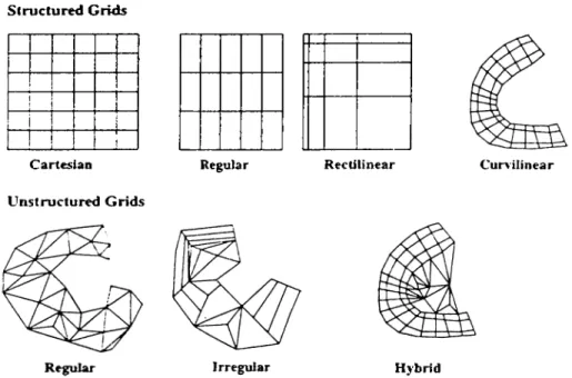
Structured Grids -4- -i-Cartesian Unstructured Grids

Regular Rectilinear Curvilinear

Hybrid

Figure 2.1: Types of grids encountered in volume rendering.

interna] cell.

The topolog}· of sample points impose a grid on the volume. Type of the grid also defines spatial characteristics of the volumetric dataset, which is im portant in the rendering process, \arious classifications of grids e.xist in the literature [7.

8

. 9. 10]. Figure

2.1

shows one of the most popular classifications of grids made by ^'agel [9]. In his work, he divides the grids into two categories which are further classified as:

• .Structured Grids - Cartesian - Regular - Rectilinear - Curvilinear • Unstructured Grids - Regular - Irregular - Hvbrid

(27)

CHAPTER 2. VOLUME RESDERI^'G: A S OVERVIEW 12

In structured grids, the sample points are distributed regularly in

3

D space. The distance between points may be constant or variable. This property is easily observed in cartesian, regular and rectilinear grids. In curvilinear grids it is not so obvious. In curvilinear grids, a structure in the distribution of sample points still exists, but is harder to capture. The sample points are distributed to fit onto a curvature in space. The cell shapes in structured grids are hexahedral cells. They have eight vertices. As these grids preserve a structure in the distribution of sample points, they can be represented by 3D arrays, therefore they are usually called array oriented grids. The mapping from the array elements to sample points in these grids is implicit, and one-to-one. Due to array oriented nature of structured grids, the connectivity relation between cells is also implicit. On the other hand, in unstructured grids the distribution of sample points do not follow a regular pattern, and there may be voids in the grid. The spacing between sample points is variable, and there exists no constraint on the cell shapes. Most common cell shapes in unstructured grids are hexahedral and tetrahedral shapes. Unstructured grids are common in engineering simulations especially in Computational Fluid Dynamics (CFD). Finite Volume Analysis (FVA). In addition, curvilinear grids are also common in CFD simulations. .Another term used for unstructured grids is cell oriented grids, because these grids are represented by a list of cells in which each cell contains pointers to sample points that form the cell. Due to the cell oriented nature and the irregularity of those grids, the connectivity information must be provided explicitly if necessary. Unstructured grids can be further divided into three subtypes as regular, irregular and hybrid. In regular unstructured grids, the cell shapes are consistent, and one face is shared between at mo't two cells. In irregular unstructured grids, there is no consistency in cell shapes, and one face can be shared by more than two cells. Hybrid unstructured grids appear as a combination of structured and unstructured grids.

2.3 Taxonomy of Volume Rendering Algorithms

(28)

CHAPTER 2. VOLUME RENDERING: AN OVERVIEW

13

• Indirect Volume Rendering algorithms (Isosurface extraction) • Direct Volume Rendering algorithms

The main aim of the algorithms that fall into the first category is to extract intermediate geometric representation of a surface from the volumetric data, and render the surface using conventional rendering techniques, whereas direct methods aim to visualize the volume directly without using intermediate ge ometric primitives. Direct methods are computationally more expensive, but give more accurate results compared to the indirect methods.

2.3.1 Indirect Volume Rendering algorithms

Isosurface extraction algorithms try to detect level surfaces throughout the volume as best as possible (a level surface is defined herein as a continuous surface within the volume such that, at each point on the surface the value of the scalar is the same [

12

]. Most of the work done on this category is for structured grids. Within this category, there are two subdivisions; first, techniques that operate on slices by applying 2D tracking algorithms and then e.xtracting a surface between consecutive contours [13. 14]; and a technique that applies an isovalue surface detector to each set of eight voxel vertices in the dataset, to produce a large set of voxel-sized polygons which are then rendered [15, 16].

In [13] contours, which are detected using an edge tracking algorithm, are used to define regions of interest in each slice. A skimming algorithm [17] is then employed to connect contours in adjacent slices to form a polygon mesh.

Both [13] and [14] are two stage methods. In the first stage, the contours are detected in the 2D slice domain, and in the second stage, adjacent slices, or contours are used for final rendering. The major problem with both of these approaches is that there is no guarantee that the tracking will detect only single contours in each slice. For example, a blood vessel which branches into two may result with one contour in one slice, and two contours in the adjacent slice. The problem becomes more difficult to handle when the distance between

(29)

CHAPTER 2. VOLİ M E RENDERING: AN OVERVIEW U

slices become large with respect to the size of cells on the slices [18]. The major deficiency of those methods arise from their non-isotropic nature in -3D space. One algorithm is used to track contours on the slices, whereas a completely different heuristic is employed to connect contours in adjacent slices.

The next approach which is called Marching Cubes Algorithm does not use slices to detect isosurfaces, but it extracts a surface directh' from the acquired data and therefore is isotropic in .3D space.

In [16], the algorithm is said to have two primary steps for surface con struction problem. In each voxel, the surface corresponding to a user-specified threshold is located, and the triangles that are formed by the intersection of surfaces and voxels are classified. After this stage, at each vertex of each tri angle the normals of surfaces are calculated, and using the gradient values isosurfaces are formed. The next stage is to display isosurfaces using conven tional rendering techniques. In his subsequent work, Lorenson introduces a new algorithm that he names as Dividing Cubes algorithm. Both Marching Cubes and Dividing Cubes algorithm produce 3D surface contours from vol ume data, the former creates triangles as primitives whereas the latter uses points with normals. In both techniques, a user specified threshold is used to select the surface to be visualized. Another important point to state is that the former is more suitable for cases w'here the number of triangles is less than the number of pixels, whereas the latter is more appropriate for cases where the number of triangles approaches the number of pixels.

In [17]. a method which supports the extraction of isosurfaces from irreg ular volume data represented in tetrahedral decomposition in optimal time is presented. The method is based on a data structure called interval tree, which encodes a set of intervals on the real line, and supports efficient retrieval of all intervals containing a given value. Each cell in the volume data is associated with an interval bounded by the extreme values of the field in the cell. .All cells intersected by a given isosurface are extracted in

0

(n? + logh) time, with n) the output size and A the number of different extreme values (min or m ax).

Isosurface extraction algorithms are very suitable for medical imaging appli cations. since they need to display multiple tissue densities and specific tissue

(30)

CHAPTER 2. VOLUME RENDERLSG: AN OVERVIEW

15

boundaries. It is possible to assign a particular color and effective opacity to each tissue in boundary based on its isodensity value. Then surface contours that define each tissue type can be used to determine the actual structure and location of the surface, its color and opacity. Contours can be made visible to varying degrees by assigning opacities according to the order of the boundaries between different tissues in the dataset.

2.3.2 Direct Volume Rendering algorithms

One of the main problems with indirect methods is that in those methods a discontinuity is forced into the data by introducing artificial surfaces. These discontinuities are highly non-linear and therefore introduce artifacts into the final image. Thus, a surface visualized in the rendered image may not reflect the actual structure of the data. Direct methods overcome this problem by assuming the volume data to be made up of small particles that emits, absorbs or reflects light depending on the lighting model used. Therefore, the images produced are like semi-transparent clouds with less artifacts.

Direct Volume Rendering (DVR) methods can be divided into two phases:

resam pling and com position phase. In resampling phase the volume is recon structed by creating imaginary sample points in the volume by making use of interpolation methods from the e.xisting sampling points. The new sam]>le points are created along the path of rays cast from each pixel into the \olume data. To create a new sample, the vertices of the cell in which the new sample will be created are used. Most approaches use Inverse Distance Inter

polation [19] to find the value of the scalar in the new sampling point. That is, first, distance of each vertex to the new sample point is calculated, and then contributions of each vertex to the sample point is calculated inverselx' to the distance of the vertex to the new sample point. Therefore, the smaller is the distance between the vertex and the new sample point, the larger is the contribution of the vertex.

In composition phase, the new interpolated samples are mapped to a color

C s and an opacity value Os by applying a m apping function, also called the

(31)

C H A PTER 2. VOLUME RENDERING: AN OVERVIEW

16

opacity value. The selection or design of transfer functions have a high impact on the resulting image, and is an area of research that is beyond the scope of this thesis. The new color and opacity values obtained are composited in either

front-to-beu:k, or back-to-front order to from the final image. In front-to-back composition, the samples are composited starting from the first sample closest to the image plane, and in back-to-front composition, the furthest sample is the first to start the composition process. If composition is performed from back-to-front, following equation is evaluated to find the composited color at a pixel

f^i+i = C iiI — Og) -f CgOg (

1

)

where C,+i is the color after compositing the new sample, Ci is the color composited from the previous sampling points, C, is the color and

0

, is the opacity· at the current sampling point both of which are obtained by application of interpolated scalar to the transfer function. Initially, a background with opacity Os = Ob = I is placed or assumed to be placed behind the volume and Cs = Cb = background color is taken as the color at starting point. For front-to-back compositions, the following equation [

20

] is evaluated to calculate the composited color at a pixel

C.+iO,+i = C , 0 . - l · C s 0 s i l - 0 , )

Oi+i = Oi Os{l — Oi) (2) where (C ,+i.O ,+i) is the (color.opacity) tuple after processing sample point. (C,. O,) is the (color .opacity) tuple before processing sample point, and (C,,. O ,) is the (color.opacity) tuple at the current sample point. Initially (To and Oo are set to zero. In both cases the composition operation is associative but iwi commutative so the order of composition is very important for the accuracy of the image. This restriction requires that either the sample points should sorted after being estimated, or they should be calculated in a sorted way.

The process of determining the cell that contains a sample point in the resampling phase is called point location problem. Sorting sample points or estimating them in a sorted order is defined as view sort problem. Both of the problems are easier to solve in structured cartesian, regular, and rectilinear grids because the regular distribution of the sample points in the volumetric

(32)

17

dataset and implicit connectivity between volume elements make these prob lems almost trivial ones to solve. However, solving point location and view sort problems in curviJine^r and unstructured grids is more difficult. In unstruc tured grids, data points (original sample points), hence cells, are distributed irregularly over 3D space. A naive algorithm may need to search all cells to determine the cell to be used in the calculation of a new sample point. This can result in very large execution times as expected. In addition, sorting sample points along a ray takes a lot of time, if not handled efficiently. Therefore, the performance of the algorithm heavily depends on the efficiency of the tech niques that are used to solve these problems. .Approaches to solve these two problems in unstructured grids are explored in more detail in Section 2.4.

We can classify direct methods into the following three categories:

• Ray casting methods • Projection methods • Hybrid methods

Ray casting methods are also called image-space methods because there is a notion of a ray which is shot from each pixel on the screen and is followed and sampled in the volume to find the contribution of the volume data onto that pixel. Projection methods are, in general, approximations to ray casting, but they are faster as they use image-space coherency in the data more efficiently. They are also called o bject-sp a ce approaches. Hybrid methods are those which process the volume data in object-space order creating spans by interpolation to find the contributions of cells.

Ray-Casting Methods

Ray casting is a popular method to construct images from volumetric data sets. In ray casting, at least one ray per image pixel into volume is cast, and is sampled along the volume with a lighting model to find the contribution of the data to that pixel in the image. It should be noted that for non-con vex

(33)

18

data sets, the raj's may enter, and exit the volume more than once. The parts of the ray that lie inside the volume, which in fact determines the contribution of data to the pixel, are referred to here as ray-segments. In this section, we will investigate the related work on ray-casting methods for structured grids.

Blinn [21] introduces the use of density models in computer graphics where he considers plane parallel atmospheres. Other researchers have adapted his models to more general shapes. Max [22] defines clouds as densities the bound aries of which are defined by analytical functions. Voss [23] fractally generates densities with a series of plane parallel models. His technique yields very re alistic images. K aji}a and Von Herzen [24] present a new algorithm to trace objects represented by densities within a volume grid. They develop light scat tering equations presenting a new approximate solution to the full-3D radiat ive scattering problem, and they compare it wdth the previous models.

Drebin e i al. [25] assumes that the measured data consists of different ma terials (e.g. skin, bone, and muscle), and that at any point in the volume the scalar represents the sum of the materials at that point. They further assume that no more than two materials can exist in a cell, so it is possible to describe each voxel with the percentage of materials within it. Using this percentage of the mixture of materials, the opacity and color of the voxels can be assigned. The method also explicitly computes certain boundaries between different ma terials within the volume based upon density gradient across voxel boundaries. .Sharp transition between materials result in large gradients. They model both surface color and opacity in this manner. Their approach does not threshold the data, since thresholding may produce unwanted artifacts. One drawback of their method is that one should provide as input till the expected material den sities. This means that either a model that assigns effective weights to voxels exist, or that one has to be very familiar with the data. Also the assumption that only two materials can be existent in a vo.xel may not always hold if the volume data is sampled at a low resolution.

.\ different approach has been taken in a series of papers by Levot' [26. 20]. The basic concept common in these works is to assign a color (in terms of red. green, and blue), and an opacity to each data point in the 3D grid, and then to compute the color of a pixel defined b}· a ray emanating from the obsen er's

(34)

CHAPTER 2. VOLUME RENDERING: AN OVERVIEW 19

eye through the image plane, and penetrating into the data. Samples may be taken at each voxel intersected by the ray, or at fixed size intervals. The advantage of their techniques over the method proposed by Drebin et al. [25] is that one does not need a density model of the dataset for the process.

Lacroute [27] introduces a new algorithm which makes use of shearing and warping transformations to render rectilinear grids. His algorithm seems to be the fastest algorithm to render rectilinear grids. He reports that a typical volume of size 256 x 256 x 256 is rendered approximately at 1 second on an R4000 Indigo machine by his Shear Warp algorithm, but his method is not applicable to unstructured grids.

Avila, Sobierajski and Kaufman [28, 29] introduce the idea of using spe cial hardware to speed up volume rendering. In [28], they present an algo rithm named PA RC (Polygon Assisted Ray-casting) which makes use of the

Z-Buffer [11] algorithm to find the closest and furthest possibly contributing cells. In [29], they revise their method by proposing a new^ technique which approximates the effects of contributing cells better.

Projection M ethods

Another way to produce the 2D image correspondent of a volumetric dataset is to find the contribution of each cell to the image. These projection methods are also known as object-space methods. [25. 30] are examples of such methods. The most important problem in projection methods is the view-sort problem that necessitates a view dependent sorting of the cells to find their contribution in the correct order. This problem is easier to solve in structured grids. This section presents the most common projection algorithms for structured grids.

Westover [31] describes an approximation technique called Splaiting. The name comes from the similarity of the technique with the action of striking snowballs to a wall. The cells are projected onto the image space, and their contribution is summed up to form the final image. He calls the contribution of each cell as footprint. Formally, his method reconstructs the signal that represents the original object, and samples it computing the image from the

(35)

resampled signal. For each vo.xel, the algorithm estimates the contribution to the image plane, its footprint, and accumulates that footprint in the image plane buffer. He shows that both front-to-back, and back-to-front composition of contributions is possible. The accuracy of his method depends highly on the correct computation of the footprints. In [-30]. he proves that for parallel projections, the footprint can be approximated by a lookup table, because it does not depend on the spatial location of the voxel itself for such projections.

Neumann and Cullip [32] introduce a new method of rendering volumes that leverages the 3D texturing hardwtire in Silicon Graphics Reality Engine workstations. Their method defines the volume data as 3D texture and uti lizes the parallel texturing hardware to perform reconstruction and resampling on polygons embedded in the texture. The resampled data on each polygon is transformed into color and opacity values and composited into the frame buffer. They introduce two alternative strategies for embedding the resampling poly gons, and discuss the benefits and trade-offs off each method. They report interactive rates of rendering such as 10 frames per second for a 128j r2S.rr28 dataset.

Hybrid M ethods

In hybrid methods, the volume is traversed in object-space and the contri bution of cells are determined by creating spans. In other words, each cell is transformed with the viewing parameters and is intersected by the planes defined by scanlines on the screen. The resulting polygons are divided into spans and by interpolation the contributions of cells are determined efficient 1\·. Upson and Keeler’s V-Buffer (Visible Buffer) algorithm is an example of the hybrid approaches for regular grids [33].

(36)

2.4 Direct Volume Rendering of Unstructured

Grids

As discussed in the previous sections, point location and view sort problems are the most important ones to solve in the rendering of unstructured grids. In this section, the methods developed to solve these problems efficient 1\· are examined. Most of the approaches use the coherence in the volume and on the image space to increase the efficienc}' of the algorithm. The former and latter types of coherencies are referred to here as object-space coherency and

image-space coherency, respectively.

The most obvious way to render an irregular grid is to resample it into a regular grid and then render it with available methods. Oppenheim and Schafer [34] survey techniques for the resampling of regular grids. The cor responding theory of irregular grids is examined in detail by Feichtinger and Grocheng [35]. One of the methods is to send rays directly into the volume and store the samples in a 3D buffer. .Another approach is to impose a regular grid on the irregular one, and interpolate the original data to the new grid. As this resampling to a regular grid will be done only once, it has a direct impact on the quality of the images produced. Although good interpolation techniques exist, they take too much time. This can be tolerated as it will only be performed once, but it turns out that accurate resampling is not only time-consuming but results in regular grids so large that the actual rendering becomes very slow. The main reason for this is that the irregular grids have cells of varying size and shape. The difference between the small cells which in fact denotes the area of interest and large cells where the precision is not so important is often very large. Therefore, an interpolation to a regular grid that preserves the accuracy and precision creates very large data sets. .Another drawback of these methods is that they generate huge empty areas as the reg ular grid has to cover the whole bounding box of the irregular grid. .Moreo\ er. the irregular data could be created in a regular way if desired, so direct ways to handle those ty^pes of grids efficiently are required. To sum up. resampling to a regular grids immense drawbacks regarding the produced data size, thé data quality, and the topolog\· information.

(37)

CHAPTER 2. VOLUME RENDERING: AN OVERVIEW >9

R ay-C asting M ethods

In this section, we will look at some of the ray-casting methods for unstructured grids. Most of these approaches try to exploit the connectivity relation available in the data to speed up the ray-casting process.

Garrity [36]. proposes an algorithm that makes use of the connectivity in formation between cells to traverse irregular grids. In his method, rays are first intersected by external faces to find the entry point of a ray into the volume. In order to further decrease the search for the first intersection, all external faces are geometrically sorted into a coarse 3D mesh. The ray is intersected with this mesh, and only the faces in the mesh locations, that are intersected by the ray, are tested for the ray intersection. Once the first entry point to the volume is determined, the rays is followed in the volume cell by cell by utilizing the connectivity information. Entry point of the ray to the next cell, which is the exit point of the ray from the current cell, is found by only considering the faces of the current cell. After an exit point is calculated, next cell that shares the face is found through the connectivity information. If the grid is a regular unstructured grid, this process is relatively faster, as one face can be shared at most by two cells. As there may be voids in the original data, when the ray exits the volume, the external faces are intersected with the ray again to find the next entrance point of the ray to the volume.

Koyamada [4] describes a fast method to traverse unstructured regular grids with tetrahedral cells. The ray-cell intersections are found by making use of the connectivity information. To find the first intersection of the ray with the volume, he projects and scan converts the external faces. To reduce the number of external faces, onl\· the front facing external faces are processed. Actually he sorts the front facing external cells, and scan converts them one by one. He uses the centroid points of the external faces for sorting which may result in a wrong sort order. Although he reports that such cases are rather rare, the fact that it can generate artifacts is a major penalty for his approach. In his work, he states that better polygon sorting algorithms such as list-priority algorithms [37] can be used to generate high qualit>· images. While scan converting an external face, he casts a ray from each pixel location

(38)

23

that is generated by the current external face, and follows it in the volume. Garrity [36] intersects all the faces with the ray as planes that grow to infinity, and chooses the minimum of the intersections as the exit point. So he tests all the faces of a cell to find the exit point. Koyamada [4] proposes a test that can directly determine if the face is intersected by the ray when applied to a face. So his method tests on the average two faces for each tetrahedral cell to determine the exit point. Moreover, he reports a direct inverse interpolation technique which allows the sampling calculations to be handled in an efficient way. .As this algorithm is one of the algorithms that this thesis is direct!} related, the details of his work are further described in Chapter 3.

Tabatabai et al. [38] describe methods to visualize volumes composed of

nonlinear elements. In his method, a set of linear equations are solved to find the intersection of a ray with a face. Again the first entrance point of a ra}· into the volume is Ccirried out by considering only the external faces. The algorithm superimposes a 2D mesh that is formed of equal sized pixel regions on the image plane, and the projected bounding boxes of the faces are used to mark the regions as regions that may possibly contain this face. Hence, the ray-face intersection is calculated by only considering the faces in a region. The next cell intersected is found by making use of the connectivity information between cells.

Friihauf [8] presents a new approach for the rendering of irregularly struc tured volume data. His method is based on casting rays through the com putational space on a nonregularly structured grid, instead of conventional!}· ray casting the physical space. This technique overcomes most of the difficul ties in sampling data along rays, since the computational space is regular bv definition. His approach is suitable especially rendering of curvilinear grids, but it is not applicable to unstructured grids as there is not a well defined computational space for such kinds of grids.

P ro je ctio n M e th o d s

Projection methods have also been investigated for unstructured grids. The common idea in all of the suggested approaches is to perform a view dependent

(39)

sort on volume elements, and find their contributions on the image plane and composite them. The methods differ either in sorting phase or in composition phcise, but unfortunately all of the suggested methods in the literature are approximations.

Max e( al. [41] present an algorithm to composite a combination of density clouds and contour surfaces. Contribution of each cell to the generic pixel is computed by analytically integrating color and opacity along the line of sight. In their work, it is reported that given a Delaunay Triangulation and a view point, a visibility ordering is alwaj's defined. In addition, thej' prove that a depth sort can be simply computed without having to manage the topological information. They use a sorting algorithm called numérica] distan ce sort to determine the correct visibility order.

P rojective Tetrabedra (P T ) technique proposed by Shirley and Tuchman [4'2] approximates the contribution each cell with a set of partially transparent tri angles. This polygon oriented method is faster than the previous pixel-orienled approach as conventional graphics hardw’are can be exploited. Their algorithm uses the MPDO [43] algorithm to determine the back-to-front ordering of tetra hedral cells. .After ordering the cells, they classify each tetrahedron according to its projected profile relative to the view’ point and they find the position of tetrahedra vertices after the projection transformation is applied. Then accord ing to the classification of the tetrahedron, they identify a set of transparent triangles that w’ill be used as an approximation to the contribution of the orig inal cell. They calculate the color and opacity values at the vertices of these triangles, and finally scan convert the triangles using a graphics workstation.

PT algorithm became very popular among projection methods, and lots of work to find better approximations and optimizations on the original algorithm have been developed. Wilhelms and Gelder [44] apply the projective tetralie- dra algorithm to curvilinear grids. Note that a cell of a curvilinear grid can be divided into five tetrahedral cells without introducing new sample points, thus preserving the original topology of the data. They also propose a m ulti-pass

blending method that reduces the visual artifacts that are a result of applying linear interpolation by graphics hardware instead of exponential interpolation.

Fast direct volume rendering of unstructured grids

FAST DlilECT VÖLUMB RENDEIING

OF UNSTP.ÜCTUS.ED GRIDS

FAST DIRECT X’OLUME RENDERING

OF UNSTRUCTURED GRIDS

By

Hakan Berk

September. 1997

6 4

1

ni

ABSTRACT

IV

ÖZET

VI

ACKNOWLEDGMENTS

Contents

1 Introduction

1

1.1

1.2

7

2 Volume Rendering: An Overview

9

21

3 Fast DVR of Unstructured Grids

30

3

6.1

3

6.2

4 Experimental Results

64

5 Conclusion

82

6 Appendix A

88

6.1

6.2

List of Figures

1

List of Tables

6

68

2

3

4

4

2

3

0.1

Chapter 1

Introduction

1

2

3

3

3

8

3

1.1

Contribution of the Thesis

4

1.8

3.2

7

1.2 Organization of the Thesis

Chapter 2

Volume Rendering: An

Overview

6

10

2.1 Volume Rendering

3

2.2 Terminology and Overview

n

8

2.1

3

2.3 Taxonomy of Volume Rendering Algorithms