WIRELESS MULTIMEDIA SENSOR
NETWORKS
a thesis
submitted to the department of computer engineering
and the institute of engineering and science
of bilkent university
in partial fulfillment of the requirements
for the degree of
master of science
By
Burcu Yargı¸co˘
glu
August, 2010
Asst. Prof. Dr. ˙Ibrahim K¨orpeo˘glu (Advisor)
I certify that I have read this thesis and that in my opinion it is fully adequate, in scope and in quality, as a thesis for the degree of Master of Science.
Prof. Dr. ¨Ozg¨ur Ulusoy
I certify that I have read this thesis and that in my opinion it is fully adequate, in scope and in quality, as a thesis for the degree of Master of Science.
Asst. Prof. Dr. Defne Akta¸s
Approved for the Institute of Engineering and Science:
Prof. Dr. Levent Onural Director of the Institute
STREAM MULTICASTING PROTOCOLS FOR
WIRELESS MULTIMEDIA SENSOR NETWORKS
Burcu Yargı¸co˘glu
M.S. in Computer Engineering
Supervisor: Asst. Prof. Dr. ˙Ibrahim K¨orpeo˘glu August, 2010
In recent years, the interest in wireless sensor networks has grown and resulted in the integration of low-power wireless technologies with cameras and micro-phones enabling video and audio transport through a sensor network besides transporting low-rate environmental measurement-data. These sensor networks are called wireless multimedia sensor networks (WMSN) and are still constrained in terms of battery, memory and achievable data rate. Hence, delivering mul-timedia content in such an environment has become a new research challenge. Depending on the application, content may need to be delivered to a single des-tination (unicast) or multiple desdes-tinations (multicast). In this work, we consider the problem of efficiently and effectively delivering a multimedia stream to mul-tiple destinations, i.e. the multimedia multicasting problem, in wireless sensor networks. Existing multicasting solutions for wireless sensor networks provide energy efficiency for low-bandwidth and delay-tolerant data. The aim of this work is to provide a framework that will enable multicasting of relatively high-rate and long-durational multimedia streams while trying to meet the desired quality-of-service requirements. To provide the desired bandwidth to a multicast stream, our framework tries to discover, select and use multicasting paths that go through uncongested nodes and in this way have enough bandwidth, while also considering energy efficiency in the sensor network. As part of our framework, we propose a multicasting scheme, with both a centralized and distributed ver-sion, that can form energy-efficient multicast trees with enough bandwidth. We evaluated the performance of our proposed scheme via simulations and observed that our scheme can effectively construct such multicast trees.
Keywords: Wireless sensor networks, Wireless multimedia sensor networks, Streaming media, Multicasting, Multicast trees.
A ˘
GLARINDA BANT GEN˙IS
¸L˙I ˘
G˙I B˙IL˙INC
¸ L˙I VE ENERJ˙I
˙IDAREL˙I VER˙I AKIS¸I C¸O ˘
GA G ¨
ONDER˙IM
PROTOKOLLER˙I
Burcu Yargı¸co˘glu
Bilgisayar M¨uhendisli˘gi,, Y¨uksek Lisans Tez Y¨oneticisi: Y. Do¸c. Dr. ˙Ibrahim K¨orpeo˘glu
Austos, 2010
Kablosuz algılayıcı a˘glarına olan ilgi yakın zamanda b¨uy¨ud¨u ve bu d¨u¸s¨uk g¨u¸cl¨u kablosuz teknolojilerin kamera ve mikrofonlarla birle¸smesiyle, d¨u¸s¨uk hızlı ¸cevresel ¨
ol¸c¨um verisi dı¸sında, g¨or¨unt¨u ve ses algılayıcı a˘glarda g¨onderilebilmeye ba¸slandı. Bu algılayıcı a˘glara, kablosuz ¸cokluortam algılayıcı a˘gları deniliyor ve pil, hafıza ve eri¸silebilir veri hızı y¨on¨unden hala kısıtlılar. Bu y¨uzden b¨oyle bir ortamda ¸cokluortam i¸ceri˘gi g¨onderimi yeni bir ara¸stırma konusu haline geldi. Uygula-maya ba˘glı olarak, i¸ceri˘gin tek bir hedefe yada birden fazla hedeflere g¨onderilmesi gerekebilir. Bu ¸calı¸smada bizler, bir ¸cokluortam veri akı¸sını birden fazla hedefe verimli ve etkili bir ¸sekilde g¨onderim problemini ele aldık, ¨ornek olarak kablo-suz algılayıcı a˘glarındaki ¸cokluortam ¸co˘gag¨onderim problemini verebiliriz. Bu a˘glarda ¨one s¨ur¨ulm¨u¸s var olan ¸co˘gag¨onderim ¸c¨oz¨umleri az bant geni¸sli˘gi kul-lanan ve gecikmeyi idare edebilen veriler i¸cin enerji verimlili˘gi sa˘glayabiliyorlar. Bu ¸calı¸smanın amacı ise, nispeten daha y¨uksek hızlı ve uzun s¨ureli ¸cokluortam veri akı¸sları i¸cin istenilen servis kalitesini kar¸sılamaya ¸calı¸san bir ¸co˘gag¨onderim sistemi olu¸sturmaktır. C¸ alı¸smamızın bir par¸cası olarak, yeterli bant geni¸sli˘gine sahip olan, enerji verimli ¸co˘gag¨onderim a˘gacı olu¸sturabilen, bir merkezi bir de da˘gıtık versiyonlu ¸co˘gag¨onderim ¸seması olu¸sturduk. Sim¨ulasyonlar aracılı˘gıyla ¨
onerdi˘gimiz protokollerimizin performansını inceledik ve sonucunda istenilen ¸co˘gag¨onderim a˘ga¸clarını etkili bir ¸sekilde olu¸sturabildi˘gini g¨ord¨uk.
Anahtar s¨ozc¨ukler : Kablosuz algılayıcı a˘glar, Kablosuz ¸cokluortam algılayıcı a˘gları, Veri akı¸sı g¨onderimi, C¸ o˘gag¨onderim, C¸ o˘gag¨onderim a˘ga¸cları.
I would like to express my gratitude to my supervisor whom I learned a lot, Assist. Prof. Dr. ˙Ibrahim K¨orpeo˘glu, for his guidance, effort, and encouragement in the supervision of the thesis. Especially I thank for his continuous morale support during this research and giving me the opportunity to work with him.
I am also indebted to Dr. ¨Ozg¨ur Ulusoy and Dr. Asst. Prof. Dr. Defne Akta¸s for showing keen interest to the subject matter and accepting to read and review this thesis.
Finally, I would like to thank to my parents and my brother Berk Yargı¸co˘glu for their support, understanding and for many things.
1 Introduction 1
2 Background Information 5
2.1 Wireless Sensor Networks . . . 5
2.2 Wireless Multimedia Sensor Networks . . . 6
2.2.1 Network Architecture . . . 6
2.2.2 Applications of WMSNs . . . 7
2.2.3 Challenges in WMSNs . . . 8
2.3 Multicasting in WMSNs . . . 10
2.4 Existing Structures . . . 12
2.4.1 Shortest Path Tree (SPT) . . . 12
2.4.2 Minimum Spanning Tree (MST) . . . 14
3 Related Work 16
4 Proposed Solution 21
4.1 Wireless Sensor Network Model . . . 21 4.2 Problem Overview . . . 22 4.3 Grouping Strategy . . . 26 4.3.1 Creating Groups . . . 27 4.3.2 Grouping Algorithm . . . 28 4.3.3 Recursive Grouping . . . 30
4.4 Centralized Stream Multicasting Protocol (CSMP) . . . 32
4.4.1 Problem Formulation . . . 32
4.4.2 CSMP Algorithm . . . 32
4.5 Distributed Stream Multicasting Protocol (DSMP) . . . 36
4.5.1 Route and Congestion Table Maintenance (RCT) . . . 37
4.5.2 RDREQ and RDREP Messages . . . 38
4.5.3 Best Path Selection between Two Relay Destination Nodes 40 4.5.4 DSMP Algorithm . . . 41
4.5.5 Summary . . . 44
5 Performance Evaluation 46 5.1 Simulation Setup . . . 47
5.2 Performance Metrics . . . 50
5.3 Evaluation of the Algorithms . . . 52
5.3.2 Success Rate . . . 54 5.3.3 Average and Maximum Delay . . . 56
6 Conclusion and Future Work 61 6.1 Conclusion . . . 61 6.2 Future Work . . . 62
2.1 A single-tier clustered, heterogeneous sensors, centralized
process-ing, centralized storage network. . . 6
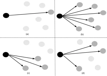
2.2 Examples of routing schemes: (a) unicast, (b) broadcast, (c) geo-cast, (d) multicast . . . 10
2.3 Examples of (a) inefficient multicast tree, (b) efficient multicast tree 11 4.1 Example 1: Destinations u,v and x,y are more likely to share sub-paths. . . 24
4.2 Example 2: Destinations u,v and x,y are more likely to share sub-paths. . . 24
4.3 Result of example 1 branching from the source . . . 25
4.4 Result of example 2 branching from the source . . . 25
4.5 Angle value θ between a source S and a destination D . . . 27
4.6 An example (a) network, (b) grouping . . . 28
4.7 An example (a) subnetwork, (b) recursive grouping process . . . . 31
4.8 Skeleton of the multicast tree formed after grouping process . . . 31
5.1 Screenshot of an example random topology with 100 nodes . . . . 48
5.2 Screenshot of an example random topology with 250 nodes . . . . 49
5.3 Rate 0.1 chart for energy consumption. . . 53
5.4 Rate 0.2 chart for energy consumption. . . 53
5.5 Rate 0.3 chart for energy consumption. . . 54
5.6 Rate 0.1 chart for success rate. . . 55
5.7 Rate 0.2 chart for success rate. . . 55
5.8 Rate 0.3 chart for success rate. . . 56
5.9 Rate 0.1 chart for maximum delay. . . 57
5.10 Rate 0.1 chart for average delay. . . 58
5.11 Rate 0.2 chart for maximum delay. . . 58
5.12 Rate 0.2 chart for average delay. . . 59
5.13 Rate 0.3 chart for maximum delay. . . 59
4.1 An example output of the grouping algorithm . . . 30
4.2 RCT: Route and Congestion Table . . . 38
4.3 RDREQ: Route Discovery Request Packet . . . 39
4.4 RDREP: Route Discovery Reply Packet . . . 40
5.1 Simulation parameters . . . 50
5.2 Parameter definitions . . . 51
Introduction
A sensor node is a tiny device that can measure and collect various data from an environment. A network consisting a set of such sensor nodes is called a wireless sensor network (WSN) and can be used in a variety of applications. Simple sensor nodes can provide environmental measurement data such as temperature, pressure and motion. They have limited energy supply, since they are usually powered by irreplacable batteries, and their processing and memory capacity is relatively lower than other mobile and wireless devices. Therefore, they need to be designed to operate very efficiently.
Sensor nodes are able to communicate using wireless interfaces with short radio range. Hence, in most scenarios intermediate nodes are used for com-munication between two nodes. A source node initially acquires data from the environment and sends the data to other nodes via the help of routing protocols which enable the messages to travel from sources to destinations using some relay nodes.
Depending on the application, routing protocols need to deliver the content to a single destination (unicast) or multiple destinations (multicast/broadcast). Unicast routing is used to send a generated data from the source node to a single destination, in most cases to the sink node. Another scenario is sending the same data to all other nodes in the network, which is called broadcasting.
Multicasting is a subset of broadcasting, in which a message is delivered from the source node to a specified set of destination nodes. Since wireless sensor networks need to be energy efficient, multicasting is a fundamental routing service for data dissemination. Compared to unicasting, multicasting is more challenging as efficient paths have to be constructed to multiple destinations to reduce overhead, and save energy.
On the other hand, with the development of the wireless technologies, cam-eras and microphones can now be integrated into sensor nodes, and in this way image, audio and video sensing also becomes possible. Such sensor networks that can sense and transport also multimedia content are called wireless multimedia sensor networks (WMSNs). Using multimedia sensor nodes in WSNs enhances the capability of an event description, hence can be used in many applications such as surveillance, monitoring, traffic enforcement, and health care delivery. Consequently these potential applications require sensor networks to receive and transmit multimedia streaming data which is a challenging task due to the limited battery, storage capacity, bandwidth and processing power of sensor nodes.
Since physical conditions such as temperature, pressure can be conveyed through low bandwidth and delay tolerant data streams, so far energy efficiency was the most significant research challenge in wireless sensor network research. However, a multimedia stream is a relatively much higher-rate and longer dura-tional data stream and some desired quality of service requirements have to be met for multimedia transmission. Therefore previous solutions in wireless sensor networks are not well suited for wireless multimedia sensor networks and they need to be re-considered to be adapted for the delivery of large data streams.
Providing efficient multicast routing in WMSNs is vital if we consider redun-dant large data streams being transmitted in an energy and bandwidth-limited network. Scarce network sources have to used wisely to construct efficient paths having minimal amount of unnecessary transmissions. However, due to the re-quirements of multimedia content, delivery of the data needs to be done with some certain level of quality of service. Energy efficiency, delay and bandwidth has to be considered together. Multimedia streaming considering these issues in
WSNs is not much investigated, as far as we know, is a challenging research issue. In this work, we address the challenge of bandwidth-aware and energy-efficient stream multicasting in wireless multimedia sensor networks. We propose a frame-work that will enable multicasting of relatively high-rate and long-durational mul-timedia streams, while trying to meet the desired quality of services. We try to provide the desired bandwidth to a multicast stream while considering energy efficiency in the network. Our framework tries to discover, select and use multi-casting paths that go through shortest uncongested nodes (i.e. paths that have enough bandwidth), while also reducing delay as much as possible and considering energy efficiency. As part of our framework, we propose a multicasting scheme forming such efficient multicast trees, with both a centralized and a distributed version.
In the construction of a multicast tree, branching which is duplicating an incoming packet to multiple neighbors, is an important factor for bandwidth, de-lay and energy consumption. Early branching may cause more timely delivery, but will consume more energy and cause more congestion. On the other side, delaying branching will increase the latency but it can use bandwidth more ef-ficiently, hence enable multicasting of large streams through the network. For these reasons, constructing routes with fewer branches where some delay is tol-erable will be the directing idea to our solution. Considering a multicast session, the source node and destination nodes have to send/receive the data, but the other nodes in the network do not have to if not required. Hence, to prevent redundant data transmissions in unrelated nodes and reduce branching, our idea is to allow branching only at source and destination nodes and try to forward the data primarily through them.
However, branching on those points along the path should be done wisely for not causing much delay. The destinations that are likely to share paths should be directed to be on the same path and vice versa. For this purpose, a grouping strategy for defining the branching points and forming the skeleton of the multicast tree is developed and used in both centralized and distributed versions of our scheme. In our centralized algorithm, the basic idea is to compute feasible
paths using known global network information in the base station. A multicast tree ensuring the required capacity for multicast sessions is computed and an initial setup process takes place informing the assigned relay nodes about the multicast session going to start. Whenever a relay node hears a packet belonging to that multicast session, it will broadcast the packet to accomplish its assigned duty.
A network formed in an ad-hoc fashion generally has no global network in-formation as it is hard to obtain and maintain. To be used in those cases where global network information is not available, we also propose a distributed pro-tocol utilized just localized information, which is requiring only the locations of the destinations to be known to the sender. Our distributed protocol constructs a multicast tree using a Route and Congestion Table (RCT) at each node, and Route Discovery Request (RDREQ) and Route Discovery Reply (RDREP) mes-sages as part of a route discovery process. A path selection between any two relay destination nodes occurs after several alternative paths are discovered. Our distributed algorithm forms up the intended multicast trees that are the same as the trees resulting from the use of our centralized protocol.
We performed extensive simulations to observe the efficiency of the multicast trees constructed by our proposed scheme. We compared our scheme with some basic tree structures that can be used for multicasting, such as shortest path trees and minimum spanning trees. We evaluate the results in terms of energy consumption, delay and success rate of the multicast transmissions. The results show that our proposed scheme can effectively construct the multicast trees.
The rest of the thesis is organized as follows: In Section 2, we give some background information, and in Section 3, we give the related work. In Section 4, we introduce and describe our distributed and centralized multicasting algorithms in detail. In Section 5, we provide the results of our performance evaluation. Finally, in Section 6 we conclude the thesis and briefly discuss some future work.
Background Information
2.1
Wireless Sensor Networks
A wireless sensor network (WSN) [3] is a network consisting of tiny sensor nodes, constrained in terms of energy and bandwidth, and spatially distributed in an area. Each node is equipped with a wireless communication module. The funda-mental objective for such a network is to cooperatively monitor physical events or conditions in an environment such as temperature, sound, pressure or motion. The sensed data is then reported to sink nodes or the base station via several nodes intermediate sensor nodes hop-by-hop, which is called multi-hop routing.
WSNs are initially developed for military applications such as battlefield surveillance but now they are widely used for monitoring, tracking, or control-ling purposes. Specific applications include habitat monitoring, industrial process monitoring and control, healthcare applications, home automation, traffic control, object tracking, and fire detection.
2.2
Wireless Multimedia Sensor Networks
Due to tremendous potential of wireless sensor networks, the research has been grown on the subject and led up to integration of low power wireless technolo-gies with cameras and microphones in recent years. Besides measuring physical phenomena and delivering scalar data, sensor nodes became capable of delivering multimedia content. These type of sensor networks are called Wireless Multime-dia Sensor Networks (WMSN) [2] and are still constrained in terms of battery, memory and achievable data rate. Hence, retrieval and transport of large data streams of video and audio in such an environment has become a new research challenge.
2.2.1
Network Architecture
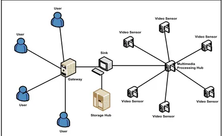
A multimedia sensor network can be in different architectures composed of several different devices. The architecture changes according to the number of tiers (single or multi), type of sensors used (homogenous or heterogeneous), processing and storage ways (distributed or centralized). An example network architecture is shown in Figure 2.1: User User User User Sink Gateway Video Sensor Video Sensor Video Sensor Video Sensor Video Sensor Video Sensor Storage Hub Multimedia Processing Hub
Figure 2.1: A single-tier clustered, heterogeneous sensors, centralized processing, centralized storage network.
Network components that can take role in a sensor network are summarized as follows:
• Video and Audio Sensors: These sensors capture video, image or sound. • Multimedia Processing Hubs: They are resposible for aggregating
multi-media streams transmitted from sensors. They have large computational resources.
• Storage Hubs: Before the data is sent to the user, these devices do fur-ther processing including data mining and feature extraction to determine important characteristics of the event.
• Sink: They are responsible for communication between a user and the net-work. It is a boundary node, located at the edge of the wireless sensor network. User queries are packaged and sent to the network from this node and filtered multimedia stream is returned back to the user via this node. More than one sink may be available in a network.
• Gateway: Connectivity between sink and users may be done via gateways. • User: Users run applications and send queries to the network to perform
monitoring tasks. Results are obtained via the returning replies.
2.2.2
Applications of WMSNs
WMSNs are varied in usage, and have potential to enable many more new appli-cations:
• Multimedia Surveillance Sensor Networks:
Existing surveillance systems can be improved with multimedia content using computer vision techniques. This technology enables a crime or a ter-rorist attack to be prevented using detection systems considering suspicious behaviors. Furthermore identifying criminals, locating missing persons and
recording events like thefts, murders, violations will be possible with this technology.
• Traffic Avoidance, Enforcement, and Control Systems:
Monitoring traffic gives opportunity to many useful applications. Traffic can be controlled and routing suggestions can be advised preventing con-gestion in the roads. Recording car accidents will result in better fault identification and by monitoring traffic violations traffic enforcement may become stronger.
• Advanced Health Care Delivery:
Health care services can be advanced by some remote medical centers that can monitor the condition of the patients. In this system medical sensors will be carried by the patients and important parameters like body temper-ature, breathing activity, blood pressure and so on can be recorded. By this way early diagnosis of diseases can be done, and in an emergency situation early medical intervention may save many lives.
• Environmental and Structural Monitoring:
Besides measuring the physical phenomena, capturing multimedia content is enabled via audio and video sensors. Forests, oceans can be monitored and researchers may interpret the observed data attracting their attention. Also civil structures like bridges or dams can be monitored for their structural health.
2.2.3
Challenges in WMSNs
Potential applications of WMSNs require sensor networks providing mechanisms delivering multimedia content which is a hard task having lots of challenges. For this reason, algorithms and protocols need to address the following issues:
• Network Lifetime: Sensor systems are powered by a power unit and they are constrained in terms of battery. Therefore energy is the scarcest resource
of sensor nodes effecting the overall network lifetime. For this reason, algo-rithms and protocols has to be developed considering lifetime maximization. Energy is also the main challenge in multimedia sensor networks. Multi-media content and streaming causes large amount of traffic to be passed through sensor nodes and therefore it is much more energy consuming com-pared to transporting scalar data.
• Resource Constraints: Besides energy constraint in sensor networks, mem-ory, processing capability and achievable data rate are also limited. Systems have to be designed regarding those issues.
• Variable Channel Capacity: Each link in the wireless network have a vary-ing capacity and attainable delay. QoS provisionvary-ing is a hard task in this environment, but definitely need to be addressed by protocols designed for multimedia communication.
• QoS Requirements: Whereas minimizing energy consumption has been the main objective in ordinary sensor networks, mechanisms to efficiently de-liver application level QoS such as bandwidth, latency and jitter should be provided in multimedia sensor networks. Multimedia content can be a snap-shot triggered with an event or can be a streaming multimedia requiring continuous data delivery.
• High Bandwidth Demand: Delivery of multimedia content, especially video streams, require high data-rate as opposed to general sensor network flows. Providing such a high bandwidth demand together with low power con-sumption and delay is another challenging, but important requirement in WMSNs.
• Poor Multimedia Source Coding Techniques: Existing video encoders are not suited for low cost multimedia sensors as they have complex processing algorithms and lead high energy consumption. Design of simple encoders need to be done to reduce the amount of data to be transmitted and stored due to processing and energy constraints.
2.3
Multicasting in WMSNs
Multicasting is a fundamental routing service for efficient data dissemination due to the limited energy availability in wireless sensor networks. Multicasting in a network can be defined as sending a same piece of information, called multicast packet, to multiple destinations, which are all members of the same multicast group that are located in different regions. The node which generates a multi-cast packet is called the source or sender. Similar to wireless sensor networks, multicasting plays an important role in typical multi-hop ad hoc networks where bandwidth is scarce and nodes have limited battery power [12].
Geocasting is a similar problem which is a special type of multicasting. Des-tinations are located within a certain region of the network and the message is delivered to all nodes in the specified region. Also, the destination specified to a source can be a region where multiple nodes are located. In general, geocast schemes try to forward the data to a node in the region and then distribute it to others in the region. Various geocasting protocols exist in the literature [14].
(a) (b)
(d) (c)
Figure 2.2: Examples of routing schemes: (a) unicast, (b) broadcast, (c) geocast, (d) multicast
grown in importance and is required as a communication primitive for proto-cols. Activities such as code and state updates, maintenance of the routes, task assignment and targeted queries are few examples that can benefit from multicas-ting. As more and more multimedia applications are conceived for wireless sensor networks, the need to support multicasting in the network becomes inevitable.
In our work, we assume destinations are not clustered in a region and can be at any point in the network. Any node can be a source node initiating a multicast session. More than one destination exists and a any node in the network can be a destination. The problem is to find a way to transmit the data generated at the source node to the specified destinations. For this purpose, additional nodes may need to be used as relays to provide connectivity to all members of a multicast session. Even when not absolutely necessary to provide connectivity, use of relays may lower overall energy consumption. The set of nodes that support a multicast session (the source node, all destination nodes, and all relay nodes) and their interconnections as a tree structure is referred to as a multicast tree.
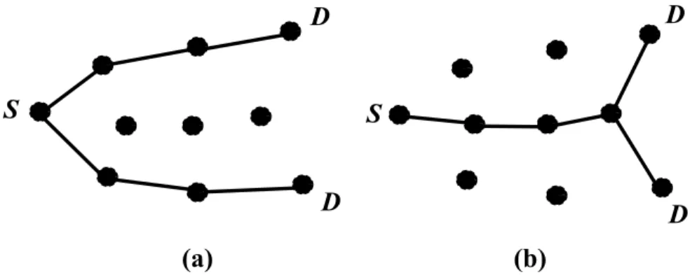
As opposed to multiple unicasting, multicasting preserves network resources by reducing redundant transmissions. Therefore, the quality of created multicast trees has a big impact on sensor networks where group communication is frequent. The establishment of a multicast tree requires a connected tree containing feasible relay nodes. A node is feasible if it has available required energy and bandwidth during the multicast session. Besides lifetime maximization, congestion in the network has to be considered when constructing such a multicast tree. Figure 2.3 shows an example inefficient and efficient multicast tree.
S
S
D
D
D
D
(a)
(b)
The nodes in any particular multicast tree do not have to use the same trans-mit power level, but in our case we assume that each node is using the same transmit power level. A constant bit rate (CBR) traffic model is assumed; thus, one transceiver is allocated to support each active multicast session at every node participating in the multicast tree throughout the duration of the session.
Multicasting in sensor networks is a well-researched topic and has many exist-ing solutions providexist-ing efficient delivery of low-bandwidth and delay-tolerant data streams with low energy consumption. But multicasting of large data streams in sensor networks is poorly investigated and has many challenges. The aim of this work is to provide a multicasting protocol considering delay, and congestion in the network besides energy efficiency. Next section gives information about some of the existing important classical structures related to multicast routing.
2.4
Existing Structures
One efficient paradigm for achieving multicast involves using spanning tree algo-rithms. The idea of these algorithms is to iteratively grow a set of covered nodes starting from the source node, and at each step, to cover one or more new nodes until all nodes in the network are covered. By this way a tree starting from the source node is built and all the receivers are spanned by that tree. A packet needs to be transported is then routed along the edges of the tree.
Several spanning tree algorithms have been developed and their performances are studied. Two classical approaches for building spanning trees are shortest path tree (SPT), and minimum spanning tree (MST) [22].
2.4.1
Shortest Path Tree (SPT)
A shortest path tree is a typical source based spanning tree algorithm. Tree formation is initiated from the source node and the constructed tree has the best unicast path to each individual destination node. Therefore, separate multicast
trees have to be computed in case of multiple senders. In the process, first an algorithm that can solve shortest path problem is applied to obtain the shortest path tree, and then the tree is oriented as a tree rooted at the source node.
2.4.1.1 Shortest Path Problem
Shortest path problem is the problem of finding a path between two vertices or nodes such that the sum of the weights of its constituent edges is minimized. An example is finding the shortest path to get from one node to another node in a network established in the Euclidean space. In this case, the vertices represent the nodes and the edge weights represent the distances among the nodes. The Euclidean distance between two points p and q is the length of the line segment connecting the points. In a three-dimensional Euclidean space, the distance can be found by the following formula:
d(p, q) =q(p1− q1)2+ (p2− q2)2+ (p3− q3)2
The most important algorithm for solving shortest path problems is the Dijk-stra’s algorithm which solves the single-pair, single-source, and single-destination shortest path problems.
2.4.1.2 Dijkstra’s Algorithm
Dijkstra’s algorithm [7] is known to be the classical algorithm that solves the single-source shortest path problem for a graph with non-negative edge weights, producing a shortest path tree. For a given source node in the graph, the al-gorithm finds the paths with the lowest costs, the shortest paths in this case, between that node and every other node. It can also be used for finding shortest paths from a source to a single destination. Therefore, Dijkstra’s algorithm is widely used in network routing protocols.
Algorithm 1 gives the pseudo-code of Dijkstra’s algorithm, which finds shortest paths from the given source node to all other nodes. In order to find one path to a destination node, one need to traverse the previous list filled in the algorithm to get one by one the nodes in the path from destination node up to the source node.
Algorithm 1 Dijkstra(G(V, E), source)
1: for all Node n ∈ V do
2: dist[n] ←∝
3: previous[n] ← undef ined
4: end for
5: dist[source] ← 0
6: Q ← ∀n ∈ V
7: while Q 6= empty do
8: current ← node in Q with smallest dist[ ]
9: if dist[current] ≡∝ then
10: break
11: end if
12: Remove current from Q
13: for all Neighbor v of n do
14: alt ← dist[n] + distBetween(n, v)
15: if alt < dist[v] then
16: dist[v] ← alt 17: previous[v] ← n 18: end if 19: end for 20: end while 21: return dist[ ]
2.4.2
Minimum Spanning Tree (MST)
Another spanning tree algorithm is the use of minimum spanning tree (MST) [9] which is a well-known greedy approach for forming a multicast/broadcast tree. A minimum spanning tree is the spanning tree of a graph which has total weight less than or equal to every other possible spanning tree of the graph. There are two commonly used algorithms, Prim’s algorithm [21] and Kruskal’s algorithm [15] to obtain an MST. The idea is to first construct the MST and then to orient it
Algorithm 2 Prim(G(V, E))
1: Pick any vertex as a starting vertex, say S. Mark it with any given colour, say red.
2: Find the nearest neighbour of S, say P1. Mark both P1 and the edge SP1 red. Find the cheapest uncoloured edge in the graph that doesn’t close a coloured circuit. Mark this edge with same colour of Step 1.
3: Find the nearest uncoloured neighbour to the red subgraph (i.e., the closest vertex to any red vertex). Mark it and the edge connecting the vertex to the red subgraph in red.
4: Repeat Step 3 until all vertices are marked red. The red subgraph is a mini-mum spanning tree.
as a tree rooted at the source node. The complexity of MST is O(n3) when a
straight-forward implementation of Prim’s algorithm is used [1]. Algorithm 2 explains how Prim’s algorithm works.
A multicasting protocol using Prim’s algorithm can use the minimum spanning tree rooted at the source node. A multicast packet can be started from the source node, and until all destination nodes receive the packet, the data packet can be led through the spanning tree. Sending of the packet at each node can be done once since all nodes are reachable via the resulting tree.
Shortest path trees and minimum spanning trees are basic tree structures that can be used for multicasting. Other relatively complex structures and protocols are explained in the next chapter.
Related Work
In this section, we briefly discuss some of the popular multicasting protocols proposed for wireless ad hoc and sensor networks. Unfortunately, majority of the research studies so far have focused on the applications requiring conventional data communication; however, these studies can be the foundations for future proposals for multimedia streaming in wireless sensor networks.
A lot of multicast routing protocols have been proposed based on different design goals and decisions. Simple solutions propose pruning approach, which produces multicast trees obtained by some spanning tree algorithms like short-est path tree (SPT) and minimum spanning tree (MST), which require global network information. Other approaches, which in general do not require global information, can be divided into two: mesh based and tree based approaches, which can be further classified into sub-categories. Protocols using local search mechanisms, greedy forwarding and geographically informed decision making al-gorithms, take their place in the current literature.
Ad hoc on demand distance vector routing (AODV) [20] is a well-known routing protocol for ad hoc networks using broadcast routing mechanism for route discovery to provide unicast communication. MAODV [6] is an extension of the AODV bringing multicast communication to the protocol. The route creation is done by route request (RREQ) and route reply (RREP) messages broadcasted
in the whole network same as in AODV. RREQs are sent as broadcasts to the whole network. When a node receives the request packet, unless it is a destination node, it rebroadcasts the packet. Each node has three route tables keeping the route information. A reverse unicast route for the node, which originally sent the request is created as entries. When the request reaches a destination, RREP is created and sent back as a unicast packet towards the source node. While traveling back, RREP establishes the selected reverse path. Continuous periodic neighbor sensing for link break detection and group hello messages are required for multicast forwarding state creation. When the source node needs to send a multicast message, it sends (as unicast) a MACT (Multicast activation) message through the selected path. Path selection is done based on hop-count, therefore in general it results with a shortest path tree (SPT) which is not the best structure for multicasting.
DSR-MB [18] utilizes route discovery mechanisms of the DSR (Dynamic Source Routing) which is a unicast routing protocol [11] for ad hoc networks. There are two main mechanisms, route discovery and route maintenance. Route discovery mechanism is similar to the AODV protocol, but with source routing instead. In DSR, when a node wishes to send a packet to another node, it employs route discovery by flooding a route request packet through the network to, search of a route to the destination. When the request reaches to a destination or to a node that has a route to that destination, it is not forwarded further. Instead, a route reply packet is sent back to the source node. The reply packet includes a full source route to the destination. When initiating a multicast, the data packet is sent within the route request packet which is then flooded in the same fashion. The target of the request is the multicast group address. Multicast group receivers make a copy of the data packet included in the route request packet and pass it up the protocol stack, before forwarding it onward. No multicast state is setup in the network for data delivery. Finally, the route maintenance mechanism monitors the status of source routes in use, detects link-failures and repairs routes with broken links.
On Demand Multicast Routing Protocol (ODMRP) [16] is a mesh-based, rather than a conventional tree-based, multicast scheme and uses a forwarding
group concept, meaning only a subset of nodes forwards the multicast packets. The nodes taking part in the multicast mesh is the forwarding group FG. The protocol builds multicast meshes through network-wide control packet floods. A periodic broadcasting of Join Request and Join Table packets are sent and received in order to form multicast mesh. Every neighbor node learns whether it is in the mesh or not by Join Table broadcasts of neighbors. By this way shortest paths to the source node are created and kept in the tables. ODMRP’s mesh structure creates richer connectivity compared to trees, therefore exploits redundant routes to overcome broken links which can be preferred in mobile ad hoc networks. But in a more static network, it will consume unneccessary energy in the nodes, especially if the data is a large and continuous stream. As a result, for our problem, ODMRP becomes an unfavourable solution.
GPSR, Greedy Perimeter Stateless Routing [13], presents a unicast routing protocol making greedy forwarding decisions using only the information about the current node’s neighbors’ positions and destination nodes’ locations in the network topology. Greedy forwarding is done by choosing the locally optimal next hop among the neighbor nodes which is the neighbor geographically closest to the destination. This closer geographic hop forwarding is done until the destination is reached. The protocol introduces perimeter forwarding, which is used in the regions where greedy forwarding cannot be used. By this way obstacles can be detoured. This protocol inspired some geographic multicasting protocols such as [19], [10], and [23].
PBM, Position Based Multicast routing [19], is one of the popular localized geographic multicast routing algorithms. It is a distributed algorithm, which tries to build a minimum cost multicast tree by applying a greedy neighbor selec-tion approach. Each relay node receiving the multicast message evaluates a cost function. By considering all possible subsets of its neighbors and assigning each destination to the closest neighbor in the subset, PBM identifies a subset which minimizes the optimization criterion. A good tradeoff exists between the total number of nodes forwarding the message and the optimality of individual paths towards the destinations. For networks with a very large number of multicast receivers, PBM may not scale well due to the need to include all destinations
in multicast data packets. Scalable Position Based Multicast for Mobile Ad-Hoc Networks (SPBM) [17] was designed to improve scalability. However, since each possible subset of the neighborhood has to be considered, both PBM and SPBM algorithm can be very costly when there are large numbers of neighbors and destinations.
Another greedy geographic multicast routing algorithm is proposed in [4], which is the most similar work to ours. Two distributed algorithms LBM-D and LBM-MST are included in the process. Firstly, considering the locations of the destinations and their angles with respect to the source node a grouping is done to reduce the branching in the multicast trees. For each group, a greedy next hop selection is done to make progress towards the destination nodes. LBM-MST calculates an Euclidean Minimum Spanning Tree once in the source node that covers all destination nodes and uses the LBM-D algorithm to follow the destinations in the constructed MST, which is distributed to the network with multicast messages. The tree formed at the end is energy efficient, but as energy efficiency is the ultimate goal, it is not suitable for multimedia streaming as it does not consider available bandwidth in the intermediate nodes.
DSM, Dynamic Source Multicast [5], is another location-based multicast routing protocol. It assumes that each node knows the geographic locations of all other nodes in the network. When a packet is to be multicast, from this known snapshot of the network, source node computes a Steiner tree [8] for the addressed multicast group using a minimum spanning tree based heuristic. The resulting multicast tree is then optimally encoded by using its unique Prfer sequence and sent with multicast packets. Each node receiving this message decodes the multicast tree that comes with the message and routes the message according to this tree. The weak point of this approach is that each node should know the location information of all other nodes in the network so as to construct the entire multicast tree. However, since the computations are performed locally, no distributed tree or mesh-like data structures are needed to be maintained among the nodes.
Geographic multicast routing (GMR) [10] exploits the wireless multicast ad-vantage to improve the forwarding efficiency of previous location-based stateless multicast protocols. Each forwarding node selects a subset of its neighbors as relay nodes towards destinations using a greedy heuristic which optimizes the cost over progress ratio. The cost is equal to the number of selected neighbors. On the other hand, the progress is calculated based on the idea of geographic for-warding, as the overall reduction of the remaining distances to the destinations. This creates a tradeoff between the cost of the multicast tree and the effectiveness of data distribution. Like GPSR and PBM, face routing is done whenever local optimum for the greedy mode is achieved. In GMR, note that each node only needs to know the locations of the destinations for which it is responsible and the locations of its one-hop neighbors; it does not require information about the topology of the whole network as DSM. However at each node testing the subsets of neighbors of a node makes the overall computational cost high as in PBM and GMP.
The underlying idea of GMP, Geographic Multicast Routing Protocol [23], is that each transmitting node constructs an Euclidean Steiner tree [8] using a reduction ratio heuristic, including the source and all destinations. Routing at each node is done according to this tree and local knowledge of neighbors. The destinations are divided into groups and a next hop for each group is selected. Then the multicast message is forwarded to that group via that node. This computation is done by all selected nodes, hence it makes GMP computationally costly. Furthermore, the constructed tree is virtual in the sense that it may include interior vertices that do not correspond to any actual wireless sensor node, so additional cost is added to deal with voids.
Proposed Solution
In this chapter, we propose and describe two new multimedia multicasting pro-tocols for wireless multimedia sensor networks. First, in Section 4.1 we discuss the wireless sensor network model that our framework considers and then in Sec-tion 4.2 we give our problem definiSec-tion and observaSec-tions in detail. Our protocols benefit from a grouping strategy, which provides energy efficiency using careful branching; in Section 4.3 we explain our grouping strategy. We describe the centralized and distributed versions of our multicasting scheme in detail in Sec-tions 4.4 and 4.5, respectively. Our scheme creates multicast trees that are both bandwidth-aware and energy efficient.
4.1
Wireless Sensor Network Model
We consider a wireless sensor network where sensor nodes are randomly dis-tributed in a field forming an ad hoc network. We assume all nodes are capable of video or audio sensing and all nodes may need to consume video or audio traffic. We assume all nodes are stationary, location-aware and have symmetric links. All nodes use the same wireless channel for communication, have the same radio range, and to not go beyond the scope, we consider the channels as being lossless.
Each node in the network can be a:
• Source node: is a node where the multicast process starts from.
• Destination node: is a node that the multicast data (stream) has to be reached to.
• Simple node: is a node which is neither a source node nor a destination node.
A destination node or a simple node can be a forwarding relay node as being member of a multicasting tree. Those nodes are called either a relay node or a relay destination node:
• Relay node: is a simple node taking place in the forwarding process to destination nodes.
• Relay destination node: is a destination node taking place in the forwarding process to other destination nodes.
For a multicast session, the set of destinations are specified to the source node with their id and location information in the network.
4.2
Problem Overview
In an energy constrained network, transmission of large data streams is a chal-lenging task. Although network lifetime is an important issue, delay and band-width are also important factors for real-time applications and multimedia. A multimedia content has to be delivered considering the energy of the nodes and at the same time considering the delivery time and bandwidth requirement of the content. Therefore, a multicast tree has to be constructed efficiently con-sidering those issues, not just with low energy consumption but also concon-sidering congestion and hop-count which provides on-time delivery.
However, delay and energy can be a trade-off. Unicasting of streams to all destinations is a simple solution on behalf of delay constraints but a sensor net-work of limited energy cannot handle this kind of an approach. Too much energy of the overall network will be consumed. This is not wise, as the same data streams will pass through multiple paths also creating congestion in the network unneccessarily. Therefore, constructing routes where some delay is tolerable for sake of energy and bandwidth efficiency will be a good idea.
In the construction of a multicast tree, branching, which means duplicating an incoming packet to multiple neighbors, is an effective factor for bandwidth, delay and energy consumption. Early branching may cause more timely delivery, but will consume more energy and cause more congestion. On the other side, delaying branching will increase the latency but it can enable multicasting of large data streams in a sensor network, since it is more energy and bandwidth efficient. For these reasons, constructing multicast routes with fewer branches where some delay is tolerable will be the directing idea in our solution.
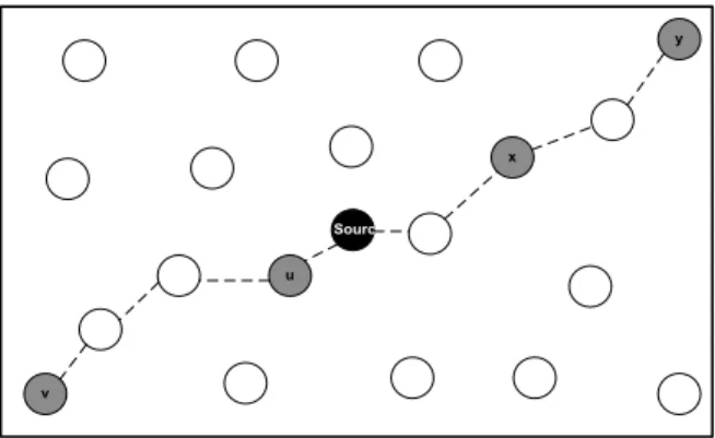
In a multicast session, the source node (i.e. the sender) or a destination node (i.e. a multicast receiver) must send/receive the data but not the other nodes. Therefore, in order to prevent unneccessary data transmissions in nodes that are neither sender nor receiver and to reduce branching, our idea is to allow branching only at the source and destination nodes and try to forward the data primarily through them. However, branching on those nodes along the path should be done wisely for not causing much delay. When there are destinations that are close to be on the same path, they should share their path.
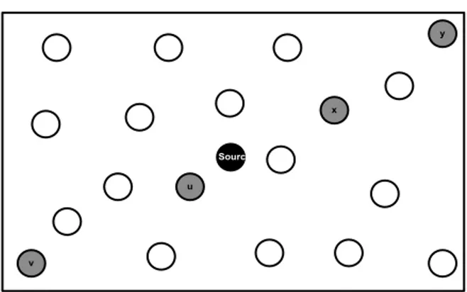
Destinations having a similar angle with respect to the source node are likely to share sub-paths. In other words, if there are large angular differences in the positions of the destinations with respect to the source node (or another desti-nation node), branching will be a good idea. Otherwise, the data may be passed through a single branch to those destinations.
Observation: When a set of destinations are positioned at a similar angle with respect to the source node, they are likely to share subpaths.
u
v
y x Source
Figure 4.1: Example 1: Destinations u,v and x,y are more likely to share sub-paths. u v y x Source
Figure 4.2: Example 2: Destinations u,v and x,y are more likely to share sub-paths.
Figures 4.1 and 4.2 show examples of our observation. In both figures, desti-nations u and v have close angular values respect to source node. Meaning that they are better reached through a same path, therefore it may be wise to group them together. The destinations x and y can also be grouped together because of the same reason.
Result: The algorithm will consider the angular differences of destinations with respect to the source node (or with respect to another destination node) when deciding to branch from the source node (or from that other destination node). u v y x Source
Figure 4.3: Result of example 1 branching from the source
u
v
y
x
Source
Figure 4.4: Result of example 2 branching from the source
If a destination is on the way to other destinations, relaying the stream on that destination and then other destinations that are likely to have common paths will help us constructing such an effective multicast tree. The algorithm should
try to route the data from the source to a group of destinations likely to have common paths. For this purpose a grouping strategy has to be defined. The next section describes how this grouping can be done.
4.3
Grouping Strategy
Grouping in our scheme is a process which takes place in every branching point, starting from the source node and then continuing at some other destinations. Firstly, the source node will find a set of destination nodes that have similar angular distance from the source node, hence can be routed on a single branch. These destination nodes will form up a group and will make up one branch coming out of the source node. Then the source node will find another set of destination nodes that will be reached via another branch out of the source. The source node will continue like this in forming groups. The number of such groups will make up how many branching will be done at the source node. Therefore, how many groups there will be may vary according to the given positions of the destinations in each multicast session and also according to the grouping criteria.
Grouping of destination nodes will be repeated on each group’s nearest des-tination node, by assigning the job similar to what the source node have done, making that destination node a relay destination node. Each such relay destina-tion node now will try to find routes to destinadestina-tions of its own group. It will first group the destination nodes specified to it by the source node. According to their angular positions, the nodes likely to have common paths are again found and the same task of finding groups is recursively assigned to the nearest destination node in each group. By this way skeleton of the multicast tree will be formed. Then the routes between the source node, relay destination nodes, and all other remaining destination nodes have to be constructed by selecting additional relay nodes from the network as forwarders of that multicast traffic. No branching is done at those relay nodes (selected from simple nodes). Branching may be done only at relay destination nodes.
4.3.1
Creating Groups
We now describe in detail our grouping method.
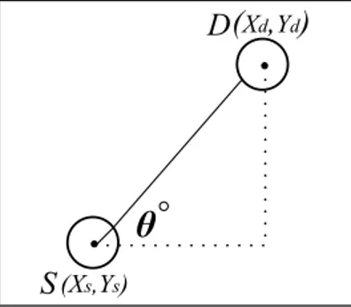
We assume a two dimensional coordinate system consisting of x-y axes, an origin and the positions of source and the destination nodes expressed by co-ordinates. Between any two nodes the angle between the x-axis and the line connecting the two points can be computed. For example, in the Figure 4.5, θ is the angle between the source node S and a destination node D.
θ
S
D(Xd,Yd)
(Xs,Ys)
Figure 4.5: Angle value θ between a source S and a destination D The angle θ can be found with the below formula:
θ = arctan( Yd− Ys Xd− Xs
)
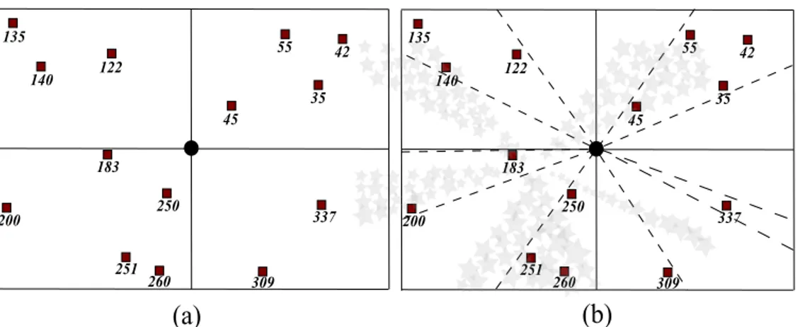
On the basis of our observation about finding sharable paths between destina-tions, we will try to group the destinations according to their θ value. The closer destinations will take place within the same group. In each group, the angle be-tween any two destinations can be at most α value which is a design choice and may change from network to network or depending on the network conditions at that time. A node that will decide branching now has to have at least two destinations having θ values with difference larger than α degrees according to this specification. However, the number of groups that will come up will vary as the θ values differ depending on the positions of destinations and each multicast session may have different number of destinations with different positions. Figure 4.6 illustrates an example about how a source node (or a relay destination node) can group some set of destination nodes.
183 200 250 251 260 309 337 45 35 42 55 135 122 140 183 200 250 251 260 309 337 45 35 42 55 135 122 140
(a)
(b)
Figure 4.6: An example (a) network, (b) grouping
4.3.2
Grouping Algorithm
The algorithm splits the given destinations into groups according to their angle values with respect to the source node or a relay destination node. We first give below the list of parameters and variables used by the algorithm:
• s: is the id of the source node.
• D: is the list of destinations to be grouped.
• α: is the maximum angle difference two nodes can have in a group.
• A: is the angle values of the nodes in the network with respect to the source node.
• S: is the sorted version of list A.
• I: is the indices in S defining starting angle values of each formed group. • m: is the index of one of two destinations having most angular gap in
between.
• N: is the group of nodes having α at most between any two nodes in a group.
Algorithm 3 GroupNodes(s, D)
1: α ← 60
2: for all Node d ∈ D do 3: A ∪ CalculateAngle(d) 4: end for 5: S ← SortInIncreasingOrder(D, A) 6: m ← FindMaxGapIndex(S) 7: I ← FindGroupStartIndices(S, m) 8: N ← GroupAll(D, α, A, S, I) 9: return N
The Algorithm 3 is our grouping algorithm. In the first line of the algorithm, α value is set to the desired value and then for each node in the destination list angle value of the node is calculated with respect to the given source node. In line 5, nodes are sorted in increasing order to find in line 6 the maximum angular gap between two destinations.After these steps, for each formed group starting angle values of them are found to place in the nodes into suitable groups in the 8th line. The node groups are returned as the last step of the algorithm.
Algorithm 4 GroupAll(D, α, A, S, I)
1: for all int i ∈ index do
2: i = 0
3: end for
4: for int k to size[D] do
5: for int m to size[I] do
6: angDif ← A[k] − S[I[m]] 7: if |angDif | ≤ α then 8: N [m] [index [m]] ← D [k] 9: index [m] + + 10: break 11: end if 12: end for 13: end for 14: return N
Algorithm 4 groups all the nodes by looking to the angular difference of each node with the group start angle values found in algorithm 3. If the difference is smaller than α in a considered group, the node is placed in that group. As a result, all nodes are located at their respective groups.
Since α is set to 60 degrees, at the end of the algorithm at most 6 groups and at least 1 group can be formed. In the given example, 4 groups are formed. For example, if the network were not having the node with angle value of 337, than 3 groups would have been formed. Table 4.1 shows the output of the algorithm at each iteration for the previous given example.
Iteration No: Formed groups with id of destination nodes It 1: (-)
It 2: (35, 42, 45, 55, 122, 135, 140, 183, 200, 250, 251, 260, 309, 337) It 3: (55, 122)
It 4: (122, 135, 140), (183, 200), (250, 251, 260, 309), (337), (35, 42, 45, 55)
Table 4.1: An example output of the grouping algorithm
4.3.3
Recursive Grouping
At a later time in the route discovery process, some destination nodes will take the job of finding the routes to a group of destinations. Those jobs are initiated firstly by the source node. Hence, the source node will be the grouping node (i.e. a relay destination node). After grouping the destinations, for each group, the job of finding routes to other desinations in that group is given to the nearest destination node in the group (that is nearest to the source node). Now, that nearest destination node will be the grouping node and grouping will be done at that node similarly, but considering only the destinations in that group (not all destinations). By this way, recursively, the branching points and how branching will be are decided, forming the skeleton of the multicast tree. Routes will be constructed afterwards between the relay destination nodes.
An example for recursive grouping is given in Figure 4.7, which is the contin-uation of the previous example.
The node having θ = 250 in the previous figure will now have a job to find routes to destinations of its own group of nodes that are 251, 260, 309 valued nodes. Same grouping procedure will be done. Now the destination nodes will
183 250 251 260 309 337 45
(a)
(b)
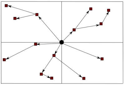
255 267 320Figure 4.7: An example (a) subnetwork, (b) recursive grouping process have different θ values with respect to current node. Grouping will result in 2 groups. 2 jobs will be assigned to node 255 and 320. Node 250 will continue this process with finding route to 267. Overall procedure will finish at node 267 and 320 as they are not responsible for finding routes to other destinations. So the relay of the streams on the whole network will be like Figure 4.8:
Figure 4.8: Skeleton of the multicast tree formed after grouping process Up to this point, we have decided the way how data streams will flow on destination nodes. In other words, we have decided where and how branching will be done starting at the source node. Now, we have to link up all the destination nodes (some of which are the branching points, i.e. relay destination nodes) to
form our multicast tree. For that purpose, we will find paths consisting relay nodes (from simple nodes, i.e. nondestination nodes) in place of the arcs shown in Figure 4.8. Next two sections describe how these relay nodes are found via our centralized and distributed protocols.
4.4
Centralized Stream Multicasting Protocol
(CSMP)
4.4.1
Problem Formulation
This protocol can be used if global network information is available at a source node. The basic idea is to use that global information in the source node and compute efficient feasible paths between relay destination nodes, ensuring the required capacity for multicast sessions. The decision about which destinations will be relay destination nodes is the result of the grouping algorithm described in the previous sections.
When paths with enough capacity are found between relay destination nodes, we have the multicast tree formed. After forming the multicast tree at the source node, an initial setup process will inform the assigned relay nodes, relay desti-nation nodes, and remaining destidesti-nations about the multicast session about to start. This knowledge can be saved as entries in a multicast session table, which is described in detail as part of our distributed protocol in the later sections. By this way, whenever a relay node receives a packet belonging to that multicast session, it will broadcast the packet to accomplish its assigned duty.
4.4.2
CSMP Algorithm
In this section, we describe in detail, how the source node computes feasible multicast paths using global information given. In the centralized algorithm, a recursive grouping and path selection is done in the source node. Initially,
the source node groups the destinations using the grouping algorithm described before. Then for each group, nearest destination among other destinations in that group is computed to find a feasible path to it. The computation of the feasible path is done with another procedure which is finding nodes with enough capacity to form a shortest path. Next, the CSMP algorithm recalls itself recursively to do the same task but this time starting from each group’s nearest destination node chosen as a relay destination node. That relay destination node now will group the destinations assigned to it and for each of its groups it will compute the feasible path to the nearest destination in that group. The algorithm resumes recalling itself until all destinations are reached.
Below are the parameters and variables used by the CSMP algorithm: - r is the current source or relay node to send data to specified destinations. - D is the specified destination list.
- c is the required capacity or stream rate for the multicast session. - V is the node list of the network.
- E is the edge list of the network.
- n is the nearest destination to the source node from every group in G. - p is the feasible path to nearest destination n.
- P is the list of feasible paths. Algorithm 5 Csmp(r, D, c, V, E) 1: G ← GroupNodes(r, D) 2: for all g ∈ G do 3: n ← NearestDestination(g) 4: p ← FeasiblePath(V, E, r, n, c) 5: P ∪ p 6: Csmp(n, g, c, V, E) 7: end for
feasible path is found, a shortest path is firstly found using Dijkstra’s Algorithm and then the path will be checked whether it satisfies the required capacity or not using IsFeasible function. If it does not satisfy, the second shortest path will be found and checked and so on. Until a feasible path is found, this procedure continues searching and returns the path if one exists. Below are the parameters and variables used by the FeasiblePath function:
- V is the node list of the network. - E is the edge list of the network. - s is the transmitter node of the path. - d is the receiver node of the path.
- c is the required capacity or stream rate for the multicast session.
- p is the shortest path from source node s to destination node d found by Dijkstra’s algorithm. Algorithm 6 FeasiblePath(V, E, s, d, c) 1: while p = nil do 2: p ← Dijkstra(V, E, s, d) 3: U ← IsFeasible(p, c) 4: if U = ∅ then 5: return p 6: else 7: remove U from V 8: end if 9: end while
Checking the shortest path whether feasible or not is done in IsFeasible method. In this method two conditions are checked in every node residing in the path. Firstly the remaining reception capacity in nodes has to be greater or equal to the required capacity by the multicast session in order to successfully receive the multicast data stream. Secondly, the nodes have to be able to forward the data, hence must have enough transmission capacity considering the required data rate. If those conditions are not satisfied then the method will return the
nodes that are not capable of being in the multicast session. During the other iteration, those nodes will not be considered anymore. Below are the parameters and variables used by the IsFeasible function:
- p is the examined shortest path.
- c is the required capacity or stream rate for the multicast session.
- U is the returned list of unavailable nodes, which have not enough bandwidth for the multicast session.
Algorithm 7 IsFeasible(p, c) 1: for all n ∈ p do 2: r ← GetReceiveCapacity(n) 3: t ← GetTransmitCapacity(n) 4: if r < c or t < c then 5: U ∪ n 6: end if 7: end for 8: return U
After the CSMP algorithm reaches to all destination nodes and stops, the multicast tree is ready to be used. To prohibit redundant information in every data packet like embedded multicast tree information the packet has to traverse, we prefer to do a setup once in the nodes for the multicast session and let every sensor node that has a job in the streaming process to know its duty. This setup can be done using a ‘Multicast Activation’ packet having the multicast session and tree information. When a node receives this message, by using a simple routing table explained as RCT table in the next section, a node can define its task as an entry belonging to that multicast session. Hence, whenever a multicast data is received, by looking to the respective entry of the multicast session, the nodes can decide to discard, transmit and process. As a result, multicast of the data streams belonging to a multimedia session can be conveyed through the network.
4.5
Distributed Stream Multicasting Protocol
(DSMP)
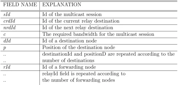
In this section, we provide a distributed protocol which is relaxing the assumption we made for our centralized algorithm and requiring the sender to know the entire network information and state. With our distributed protocol, the sender does not have to know the entire network topology and the current traffic load of the nodes. Our distributed stream multicasting protocol constructs bandwidth-aware and energy-efficient multicast trees by doing discoveries via request packets and selecting the feasible paths afterwards. Throughout this process, our distributed protocol uses a Route and Congestion Table (RCT) at each node, route discovery request (RDREQ) messages and route discovery reply (RDREP) messages. In the next sections, we explain how this route discovery process is done, how the format and the usage of the RCT is established and we describe how best path selection between two relay destination nodes is done. Finally, we give the algorithms forming up our distributed protocol.
The source node initially does not know any global information about the nodes in the network and their states, except the multicast destinations and their locations. Therefore, a local path search process is considered to collect infor-mation about nodes and their states and perform path selection in a distributed manner. The first decision is to decide on the branching points which are selected to be the relay destination nodes. As explained in the previous sections, in or-der to achieve minimum energy consumption in the network and less end-to-end delay in the transport of the data from source to destinations, branching is an important factor and should be done wisely. For this purpose, we use again the same grouping strategy we described and used in our centralized algorithm. The difference is that, now in our distributed protocol every relay destination node makes this decision, not only the source node. Initially, the source node makes de-cision about branching. Then this dede-cision making responsibility is firstly by the source node to suitable relay destination nodes, and then from those to other re-lay destination nodes. In this branching is performed and multicast tree skeleton is formed. Route request (RDREQ) messages are used for this decision making
assignment, which explained in detail in next sections.
After deciding on the branching and relay destination nodes, routes between relay destination nodes have to be constructed. The decision for the path between two relay destination nodes (i.e. between previous and next destination relay nodes) is made by the next destination relay node, when one or more route request messages have arrived to it from the previous relay destination node following different paths. The selection of path is done considering congestion level in the candidate nodes. Then route setup for a session is done by a reply message returning back from the next relay destination node to the previous relay destination node (or the source node). This forms the forward and reverse paths between two relay destination nodes using a Route and Congestion Table (RCT), which is explained in the next section.
4.5.1
Route and Congestion Table Maintenance (RCT)
Every node will maintain a route and congestion table (RCT) having multicast session information going on through itself. SessionId will be the id number of the multicast session. PreviousDestinationId and NextDestinationId numbers are the id numbers of the previous and the next relay destination nodes. Previous-DestinationId can be the source node’s id number if the forwarding node takes place between the source node and a relay destination node. ReverseHopId will be the node which the Request message has come from and the NextHopId will be the node which the Reply message have come from.
For a multicast session we will have a Status field in the corresponding entry in the RCT table. The status field can be set to one of the following values:
• Active • Waiting
• Active Destination • Waiting Destination