MODELING TURKISH M2 BROAD MONEY
DEMAND: A PORTFOLIO-BASED APPROACH USING
IMPLICATIONS FOR MONETARY POLICY
Cem SAATÇİOĞLU*
Levent KORAP**
Abstract
In this paper, a money demand model upon M2 broad monetary aggregate for the Tur-kish economy is examined in a portfolio-based approach considering various alternative cost measures to hold money. Employing multivariate co-integration methodology of same order integrated variables, our estimation results indicate that there exists a theoretically plausible co-integrating vector in the long-run money demand variable space. The main alternative costs to demand for money are found as the depreciation rate of domestic currency and the course of equity prices, for which the former brings out the importance of currency substitu-tion phenomenon settled in the economy. Besides, we find that domestic inflasubstitu-tion carries a weakly exogenous characteristic and conclude that the main factors leading to the domestic inflation are determined out of the money demand variable space.
Key words: Broad Money Demand; Co-integration; Currency Substitution; Turkish Economy.
Özet
Bu çalışmada, Türkiye ekonomisi için M2 geniş kapsamlı parasal büyüklüğü üzerine kurulan bir para talebi modeli elde para tutumuna karşı çeşitli almaşık maliyet unsurları dik-kate alınarak portföy temelli bir yaklaşım içerisinde incelenmektedir. Aynı dereceden bütün-leşik değişkenlerin çok değişkenli eş-bütünleşim tahmin yöntemi kullanılarak incelenmesi şeklinde elde ettiğimiz tahmin sonuçları uzun dönem para talebi değişken uzayı içerisinde kuramsal beklentilerle uyumlu eş-bütünleşik bir vektörün bulunduğunu göstermiştir. Para talebine karşı başlıca almaşık maliyet unsurları ekonomi içerisinde yerleşik para ikamesi olgusunun önemini ortaya koyan yerli paranın değer kayıpları ve hisse senedi fiyatlarındaki gelişmeler şeklinde bulunmuştur. Ayrıca, bulgularımız yurtiçi enflasyonun zayıf dışsal bir özellik taşıdığını göstermiş ve yurtiçi enflasyona yol açan temel etkenlerin para talebi değiş-ken uzayı dışında belirlendiği sonucuna ulaşılmıştır.
Anahtar kelimeler: Geniş Para Talebi; Eş-bütünleşim; Para İkamesi; Türkiye Ekonomisi.
* Asst. Prof. Dr., Istanbul University, Department of Economics, 34452 Beyazıt, Istanbul, Turkey. ** Economist, Marmara University, Department of Economics, Istanbul, Turkey.
Introduction
Design of monetary policy for stabilization purposes needs to extract the knowledge of various functional relationships conditioned upon possible discretionary policy tools. Inferences dealing with monetary policy will meet the stylized facts of the economy only if they succeed in constructing foresights consistent with behavioral preferences of the economic agents dominated in the economy and to the extent that such an issue of interest for policy makers can be implemented, ex-post realizations of economics policies will be expected to converge to the ex-ante expectations of the economic agents.
A useful and widely-used way of analyzing the monetary policy is to examine what pecularities the demand for monetary balances have in the eyes of economic agents and such an analysis can in this manner bring out the pre-requisites in applying to the stabilization programs which requires that app-ropriate tools be chosen to achieve program targets. These will enable policy makers to form policy rules against major economic problems such as the domestic inflationary framework or the role and the extent of currency subs-tituon in the economy as well as the general outlook of what alternative costs against holding money are mainly chosen by the economic agents. Thus, testing a standard money demand equation can provide policy makers with the crucial knowledge of expectations in the monetary markets.
For the empirical purposes, two approaches can be attributed for the behavioral assumptions leading economic agents to demand for money, i.e., the transactions and the asset or portfolio balance approaches. The transactions motives emphasize mainly the money’s role as a medium of exchange, and the demand for monetary balances in this approach increases proportionally with the volume of transactions in the economy. However, the portfolio balance approaches consider that people hold money as a store of value and money is only one of the assets among which people distribute their wealth. For the portfolio motives, people consider mainly the the expected rate of return for the various assets held in hand relative to the transactions necessities and take into account the risk factor for these assets because of the changing ratio of returns against each other. Of course, more condensed on portfolio approach, more intruments would be necessary for economic agents to hold in hand.
Given the importance of a stable money demand relationship carrying the knowledge of monetary policy issues, many papers in recent years are conducted by the researchers upon various country cases, such as Sriram (1999), Civcir (2000), Nachega (2001), Kontolemis (2002) and Dreger et al.
(2006). On the other side, papers by the CBRT researchers such as Mutluer and Barlas (2002), Akinci (2003) and Altinkemer (2004) can be considered some recent works upon the Turkish economy. In our paper, our aim is to construct a portfolio-based money demand model as a function of large set of alternative costs to hold money in the Turkish economy. For this purpose, the next section is devoted to the data issues and model specification and the third section conducts an empirical analysis for the Turkish economy, while the last section concludes.
1. DATA and METHODOLOGY
1.1. Model Construction and DataWe now construct a model of money demand for the investigation pe-riod of 1987Q1-2006Q4 using quarterly observations. While investigating the demand function, a critical point to be considered is the identification problem which means the non-observability of the money demand. As is generally assumed, for empirical purposes, researchers make on this point an important assumption that the quantity of money supplied and demanded equal each other thus assuming long-run equilibrium in the money market (Laidler, 1993). For transactions purposes, we can suppose that narrowly defined monetary variables are better to be considered, while broadly defined monetary variables used in this paper would be better off for the portfolio balance approaches in the money demand equation. After defining the money demand variable, we need to choose the explanatory factors that affect why economic agents hold monetary balances or that discourage people to hold these balances. We must first choose the scale-income variable which specifies the maximum limit of money balances people can hold in a positive relationship with money balances. Then what is of special concern for us is to determine what alternative costs against holding money are current in the economy. Finally, in order to assume a complete functional money demand relationship, the own rate of return for the money balances considered should be included in the functional form of money demand, which requires a positive relationship with money balances.
For empirical purposes, the monetary variable we used (m/p) is the M2 broad monetary aggregate including currency in circulation plus demand and time deposits in the banking system excluding the foreign currency based deposits. Under the assumption of no money illusion, we suppose that demand
for money is a demand for real money balances. In our case, we use the GDP-deflator to deflate the broad money supply. For the scale-income variable, the real gross domestic product data (y) is used. Following the general specification in Friedman (1956), the alternative cost variables to hold broad money balances in our paper are the maximum rate of interest on the Treasury bills (rtb) rep-resenting the financial assets, whose maturity are at most twelve months or less, the quarterly domestic inflation (p) based on the GDP-deflator for the expected return on real assets, which represents the increase of prices of intangible assets under the assumption of substitution between commodities and domestic money, and the Istanbul Stock Exchange (ISE) National-100 index (req) to represent the effect of equity prices on money demand. For the equity prices variable, Friedman proposes three alternative forms to be con-sidered, that is, the constant nominal amount agents would receive in a given time period in the absence of any change in p, the increment or decrement to this nominal amount to adjust for changes in p and any change in the nominal price of the equity over time. In our paper, a similar variable specification similar to the first alternative is used given the time series characteristics of the variables below.
Choudhry (1995) emphasizes that a significant presence of the rate of change of exchange rate in the demand function for real money balances may provide evidence of currency substitution in high inflation countries, which reduces domestic monetary control by also reducing the financing of deficit by means of seigniorage and the base of the inflation tax. He indicates that for three high inflation countries, i.e., Argentina, Israel and Mexico, stationary long run money demand relationship only holds with the inclusion of currency depreciation in the money demand function. Since the Turkey is a small open economy with a highly liberalized capital account, such a consideration for the alternative costs to hold money may be crucial for the economic agents. Indeed, the proportion of foreign exchange based accounts in the Turkish banking system grows from 16% in 1987 till 57% by the end of 2001 and 35% by the end of 2006, which reflects a great deal of dollarization and currency
substitution for the Turkish economy1. Following Civcir (2000), we include
1 Giovannini and Turtelboom (1992), Yılmaz (2005) and Civcir (2005) touch on the difference between the terms dollarization and currency substitution in the sense that in high inflation countries foreign currency is first used as a store of value or unit of account representing dollar-ization and only at the later used as a medium of exchange. That is, currency substitution is the last stage of the dollarization process. But, for our estimation purposes in this paper, we can ig-nore such a theoretical distinction.
expected exchange rate depreciation (e) into our model construction to represent the currency substitution. For this purpose, we first ran a regression of producer price index- (PPI-) based real exchange rate series, for which an increase means appreciation of the domestic currency, on a constant and trend and then calculated the deviation of the actual series from the predicted series for real exchange rate misalignment. Civcir also argues that expected exchange rate depreciation adjusted for foreign interest variable would be highly collinear with expected exchange rate depreciation. Besides, when we include the foreign interest variable in our money demand model separately, we find that this variable yields results with an unexpected positive wrong sign. Given also that the foreign interest data take highly trivial values when compared with the relevant Turkish data, no such an adjustment is assumed in this paper. Finally, the own rate of return for the broad money balances is represented by the three-month time deposit rate (rown).
All the data indicate seasonally unadjusted values and are in their natural logarithms except the both interest rate variables and domestic inflation which are in their linear-forms, while no impulse-dummy variable is considered. They are collected from the electronic data delivery system of the Centrak Bank of the Republic of Turkey (CBRT).
This model construction can be expressed in a functional form with appropriate expected signs such as Eq. 1 and Eq. 2 below:
m/p = f (y, rtb, p, req, e, rown) (1) or in log-linear form:
m-p =
α
+β
y -δ
rtb -φ
p -γ
req -η
e +φ
rown +ε
(2) whereε
is assumed to be a white-noise error term.1.2. Unit Root Characteristics
We now investigate the time series properties of the variables. Spurious regression problem analysed by Granger and Newbold (1974) indicates that using non-stationary time series steadily diverging from long-run mean will produce biased standard errors, which causes to unreliable correlations within the regression analysis leading to unbounded variance process. In this way, when a non-stationary I (d) process identifies any time series, the standard OLS regression in the level form will possibly produce a good fit and predict statistically significant relationships between the variables where none really
exists (Mahadeva and Robinson, 2004). This means that the variable must be differenced (d) times to obtain a covariance-stationary process. Therefore, individual time series properties of the variables should be elaborately con-sidered. Dickey and Fuller (1979) provide one of the commonly used test methods known as augmented Dickey-Fuller (ADF) test of detecting whet-her the time series are of stationary form. However, Elliot et al. (1996) pro-pose a more powerful modified version of the ADF test in which the data are detrended so that explanatory variables are taken out of the data prior to running the test regression. Elliot et al. (1996) define a quasi-difference of Xt
that depends on the value α representing the specific point alternative against which we wish to test the null:
Xt if t = 1
d (Xt⏐α) = (3)
Xt - αXt-1 if t > 1
An OLS regression of the quasi-differenced data d (Xt⏐α) on the
quasi-differenced d (Zt⏐α) yields:
d (Xt⏐α) = d (Zt⏐α)′δ (α)+ηt (4)
where Zt consists of deterministic constant or constant and trend terms
and let δ (α) be the estimated value from an OLS regression. For the value of α, Elliot et al. (1996) consider:
1 – 7/T if Zt = {1}
α = (5)
1 – 13.5/T if Zt = {1, t}
Following these specification issues, generalized least squares (GLS) detrended data Xtd are:
The DFGLS substitutes the GLS detrended Xtd data for the original Xt
data in the ADF equation. While the DFGLS t-ratio follows a Dickey-Fuller
distribution in the constant only case, the asymptotic distribution differs when included both a constant and trend. Elliot et al. (1996) simulate the critical values of the test statistic in this latter setting for T = {50, 100, 200, ∞}. We report below in Tab. 1 the DFGLS estimation results:
Table 1: Unit root tests
Variable Levels First differences
τC τT τC τT m/p y rtb p req e rown -0.55 1.82 -1.87 -1.90 1.10 -1.86 -1.87 -1.19 -1.50 -2.50 -2.35 -1.97 -3.09 -2.33 -2.71* -2.93* -8.66* -0.55 -5.63* -9.76 -8.37* -11.16* -8.43* -8.98* -9.52* -6.86* -10.02 -8.49* 1% cri. val. -2.60 -3.68
Above, τC and τT are the test statistics with allowance for only constant
and constant&trend terms in the DFGLS unit root tests, respectively, while ‘*’
means that the data are of stationary form. All the variables in the level form are found to have a unit root, however the null hypothesis that there is a unit root can easily be rejected when we apply to the differencing. Note that do-mestic inflation is trend-stationary. Besides, multivariate statistics for testing stationarity obtained from co-integration methodology below verify these findings.
1.3. Methodology
Let us assume a zt vector of non-stationary n endogenous variables and model this vector as an unrestricted vector autoregression (VAR) involving up to k-lags of zt:
zt =
Π
1zt-1 +Π
2zt-2 + … +Π
kzt-k +ε
t (7)where
ε
t follows an i.i.d. process N (0,σ
2) and z is (nx1) and theΠ
i an (nxn) matrix of parameters. Eq. 7 can be rewritten leading us to a vector error correction (VEC) model of the form:Δzt =
Γ
1Δzt-1 +Γ
2Δzt-2 + … +Γ
k-1Δzt-k+1 +Π
zt-k +ε
t (8) whereΓ
i = -I +Π
1 + … +Π
i (i = 1, 2, …, k-1) (9)and
Π
= I -Π
1 -Π
2 - … -Π
k (10)Eq. 8 can be arrived by subtracting zt-1 from both sides of Eq. 7 and col-lecting terms on zt-1 and then adding - (
Π
1 - 1)Xt-1 + (Π
1 - 1)Xt-1. Repeating this process and collecting of terms would yield Eq. 8. This specification of the system of variables carries on the knowledge of both the short- and long-run adjustment to changes in zt, via the estimates ofΓ
i andΠ
. Following Harris (1995),Π
=αβ′
whereα
measures the speed of adjustment coefficient of particular variables to a disturbance in the long-run equilibrium relationship and can be interpreted as a matrix of error correction terms, whileβ
is a matrixof long-run coefficients such that
β′
zt-k embedded in Eq. 8 represents up to (n-1) cointegrating relations in the multivariate model which ensure that zt converge to their long-run steady-state solutions. Note that all terms in Eq. 8 which involve Δzt-i are I (0) whileΠ
zt-k must also be stationary forε
t ~ I (0) to be white noise of an N (0,σ
ε2) process.For the lag length of unrestricted VAR, we consider sequential modified LR statistics which compare the modified LR statistics to the 5% critical values starting from the maximum lag, and decreasing the lag one at a time until first getting a rejection. In our case, reduction of system is first rejected when we test the reduction to 3 lag orders. Thus we construct the unrestricted VAR model with 4 lags. We add a set of centered seasonal dummies which
sum to zero over a year as exogeneous variable. In this way, the linear term from the dummies disappears and is taken over completely by the constant term, and only the seasonally varying means remain (Johansen, 1995). As a next step, we estimate the long run co-integrating relationships by using two likelihood test statistics known as maximum eigenvalue for the null hypothesis of r versus the alternative of r+1 co-integrating relations and trace for the null hypothesis of r co-integrating relations against the alternative of n co-integrating relations, for r = 0, 1, ..., n-1 where n is the number of endogenous variables.
2. RESULTS
Following the model specification expressed above, we give below the co-integration test results of the money demand model in which no deterministic trend is restricted:
Table 2. Co-integration tests
Null hypothesis ı= 0 r≤1 r≤2 r≤3 r≤4 r≤5 r≤6 Eigenvalue λ trace 5% cri. val. λ max 5% cri. val. 0.50 159.8* 125.6 51.78* 46.23 0.40 108.0* 95.75 37.46 40.08 0.36 70.57* 69.82 33.05 33.88 0.25 37.52 47.86 21.24 27.58 0.14 16.27 29.80 10.85 21.13 0.07 5.42 15.49 5.19 14.26 0.01 0.23 3.84 0.23 3.84 * denotes rejection of the hypothesis at the 0.05 level.
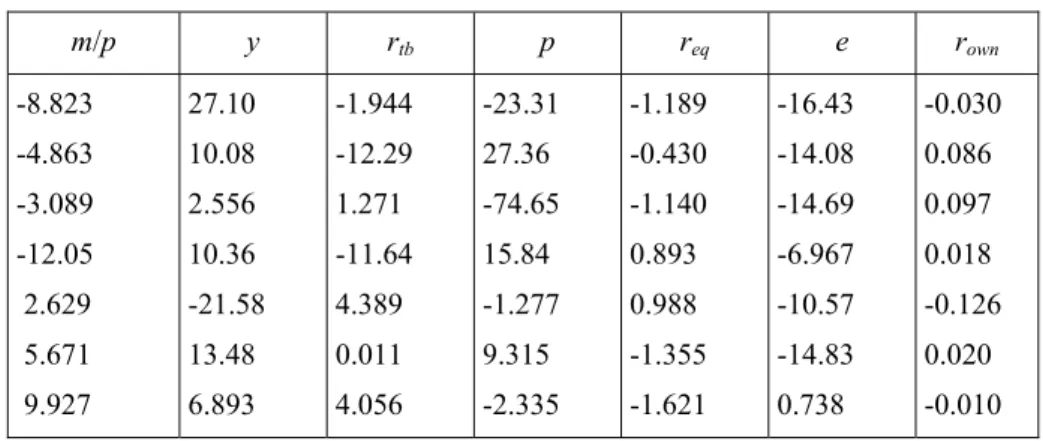
Unrestricted Co-integrating Coefficients
m/p y rtb p req e rown -8.823 -4.863 -3.089 -12.05 2.629 5.671 9.927 27.10 10.08 2.556 10.36 -21.58 13.48 6.893 -1.944 -12.29 1.271 -11.64 4.389 0.011 4.056 -23.31 27.36 -74.65 15.84 -1.277 9.315 -2.335 -1.189 -0.430 -1.140 0.893 0.988 -1.355 -1.621 -16.43 -14.08 -14.69 -6.967 -10.57 -14.83 0.738 -0.030 0.086 0.097 0.018 -0.126 0.020 -0.010
1 Co-integrating Equation (t-stat. in parantheses) m/p y rtb p e req rown Constant 1.000 -3.071 0.220 2.642 1.862 0.135 0.003 19.85 (-4.69) (1.07) (1.80) (3.33) (2.75) (1.06) Adjustment coefficients m/p y rtb p e req rown -0.077 -0.002 -0.131 -0.046 -0.050 -0.354 -0.207 (0.04) (0.03) (0.20) (0.06) (0.06) (0.18) (-0.11)
Multivariate Statistics for Testing Stationarity
m/p y rtb p e req rown
χ2 (6) 29.97 30.56 42.33 33.80 47.57 29.91 44.66
In Tab. 2, we find that trace test indicates 3 and max-eigen test 1 poten-tial co-integrating vectors lying in the long-run variable space. When we examine the unrestricted co-integrating coefficients in Tab. 2 above, we find that the first vector with the largest eigenvalue seems to be a theoretically plausible money demand vector. Thus, we accept that this vector which is found common to represent a long-run stationary relationship by both rank statistics is the money demand vector we search for. Rewriting the normali-zed money demand equation under the assumption of r = 1 yield in Eq. 10 below2:
β′
m1zt-k= m/p-3.07y+0.22rtb+2.64p+1.86+0.14req+0.01rown+19.85 (11) The results from Eq. 11 reveal that income elasticity of money demand for the real broad money balances is above unity indicating a monetization2 When the deterministic trend is restricted in the co-integrating space, we find highly similar estimation results to those with no deterministic trend, but the adjustment coefficient on real money balances turns out to be statistically insignificat in this case. These results not reported here to save space are available upon request.
process in the economy. We estimate that the unit income homogeneity rest-riction is rejected through
χ
2 (1) = 10.63 against theχ
2 (1)-table value 3.84. All the alternative cost variables have the expected normalized sign, but the sta-tistical significance can only be achieved for the currency substitution and equity price variables. The domestic inflation has also a significance in the margin for the acceptable levels. The t-statistics indicate that as for the signi-ficance levels, the main alternative cost for the economic agents to hold bro-adly defined monetary balances is the depreciation rate inside the period examined. This brings out the importance of an ongoing currency substitution phenomenon settled in the economy when the economic agents make their decisions for their monetary holdings. Besides, we find that for the feedback effects correcting disturbances from the steady-state functional form in the long-run, real income, Treasury bill rate, inflation rate and currency depreciation rate have a weakly exogenous characteristic in the money demand variable space, but the adjustment coefficients of real money balances, equity prices and own rate of return are found statistically significant. As Sriram (1999) emphasizes, in the case of negative significant error correction term of the money demand equation, a fall in excess money balances in the last period would result in higher level of desired money balances in the current period, that is, it is essential for maintaining long run equilibrium to reduce the existing disequilibrium over time. About 8% of the adjustment in money demand disequilibrium conditions to achieve long run static equilibrium is realized within one period. Multivariate statistics for testing stationarity are in line with the DFGLS unit root test results obtained above in the sense that no variablealone can represent a stationary relationship in the co-integrating vector. An important policy conclusion can also be extracted from the Tab. 2 such that no dynamic vector error correction model upon domestic inflation is warranted to be constructed, which can be derived from the money demand co-integrating vector. Such a case would mean that the main factors leading to the domestic inflation are determined out of the money demand variable space considered in this paper. Finally, the model has good diagnostics and fits well to the data generating process in the VEC model using LM (1) = 48.61 (prob. 0.49), LM (4) = 60.25 (prob. 0.13), where LM (1) and LM (4) are the 1st and 4th order VEC system residual serial correlation lagrange multiplier
statistics under the null of no serial correlation. For the VEC system residual serial correlation test, probs. come from
χ
2 (49).Concluding Remarks
In this paper, we construct a portfolio-based money demand model upon the Turkish economy employing contemporaneous multivariate co-integration methodology of the same order integrated variables. Our estimation results indicate that income elasticity of money demand for the real broad money balances is above unity indicating a monetization process in the economy. Among the various alternative cost variables, the most statistically significant one is the depreciation rate which brings out the importance of currency substitution phenomenon settled in the economy. Equity prices are also find another main alternative cost variable to hold monetary balances. Besides, we find that domestic inflation is weakly exogenous and conclude that the main factors leading to the domestic inflation are determined out of the mo-ney demand variable space.
References
Akinci, O. (2003). “Modeling the Demand for Currency Issued in Turkey”, Central Bank Review, 1, 1-25.
Altinkemer, M. (2004). “Importance of Base Money Even When Inflation Targeting”, CBRT Research Department Working Paper, No. 04/04.
Choudhry, T. (1995). “High Inflation Rates and the Long-Run Money Demand Function: Evidence from Cointegration Tests”, Journal of Macroeconomics, 17 (1), 77-91. Civcir, I. (2000). “Broad Money Demand, Financial Liberalization and Currency Substitution
in Turkey”, ERF Seventh Annual Conference Proceedings.
Civcir, I. (2005). “Dollarization and Long-Run Determinants in Turkey”, Research in Middle East Economics, 6, 201-232.
Dickey, D.A. and Fuller, W.A. (1979). “Distribution of the Estimators for Autoregressive Time Series with a Unit Root”, Journal of the American Statistical Association, 74, 427-431.
Dreger, C., Reimers, H.-E. and Roffia, B. (2006). “Long-Run Money Demand in the New EU Member States with Exchange Rate Effects”, European Central Bank Working Paper Series, No. 628, May.
Elliott, G., Rothenberg, T.J. and Stock, J.H. (1996). “Efficient Tests for an Autoregressive Unit Root”, Econometrica, 64, 813-836.
Friedman, M. (1956). “The Quantity Theory of Money - a Restatement”, M. Friedman (ed.), Studies in The Quantity Theory of Money, The University of Chicago Press, 3-21.
Granger, C.W.J. and Newbold, P. (1974). “Spurious Regressions in Economics”, Journal of Econ6ometrics, 2/2, 111-120.
Giovannini, A. and Turtelboom, B. (1992). “Currency Substitution”, NBER Working Paper, December, 4232.
Harris, R.I.D. (1995). Using Cointegration Analysis in Econometric Modelling, Prentice Hall. Johansen, S. (1995). Likelihood-based Inference in Cointegrated Vector Autoregressive
Mo-dels, Oxford University Press.
Kontolemis, Z.G. (2002). “Money Demand in the Euro Area: Where Do We Stand (Today)?, IMF Working Paper, No. 02/185.
Laidler, D.E.W. (1993). The Demand for Money: Theories, Evidence and Problems, 4. ed. New York: Harper Collins Collage Publishers.
Mahadeva, L. and Robinson, P. (2004), “Unit Root Testing to Help Model Building”, A. Blake and G. Hammond (eds.), Handbooks in Central Banking, Centre for Central Banking Studies, Bank of England, No. 22, July.
Mutluer, D. and Barlas, Y. (2002). “Modeling the Turkish Broad Money Demand”, Central Bank Review 2, 55-75.
Nachega, J.-C. (2001). “A Cointegration Analysis of Broad Money Demand in Cameroon”, IMF Working Paper, WP/01/26.
Sriram, S.S. (1999). “Demand for M2 in an Emerging-Market Economy: An Error-Correction Model for Malaysia”, IMF Working Paper, WP/99/173.
Yılmaz, G. (2005). “Financial Dollarization, (De)dollarization and the Turkish Experience”, TEA Discussion Paper, 2005/6.