IMPLEMENTATION OF PHYSICAL
THEORY OF DIFFRACTION FOR RADAR
CROSS SECTION CALCULATIONS
a thesis
submitted to the department of electrical and
electronics engineering
and the institute of engineering and sciences
of bilkent university
in partial fulfillment of the requirements
for the degree of
master of science
By
Alper K¨
ur¸sat ¨
Ozt¨
urk
July 2002
I certify that I have read this thesis and that in my opinion it is fully adequate, in scope and in quality, as a thesis for the degree of Master of Science.
Prof. Dr. Ayhan Altınta¸s(Supervisor)
I certify that I have read this thesis and that in my opinion it is fully adequate, in scope and in quality, as a thesis for the degree of Master of Science.
Prof. Dr. Hayrettin K¨oymen
I certify that I have read this thesis and that in my opinion it is fully adequate, in scope and in quality, as a thesis for the degree of Master of Science.
Dr. Vakur B. Ert¨urk
I certify that I have read this thesis and that in my opinion it is fully adequate, in scope and in quality, as a thesis for the degree of Master of Science.
Dr. Satılmı¸sTopcu
Approved for the Institute of Engineering and Sciences:
Prof. Dr. Mehmet Baray
ABSTRACT
IMPLEMENTATION OF PHYSICAL
THEORY OF DIFFRACTION FOR RADAR
CROSS SECTION CALCULATIONS
Alper K¨
ur¸sat ¨
Ozt¨
urk
M.S. in Electrical and Electronics Engineering
Supervisor: Prof. Dr. Ayhan Altınta¸s
July 2002
A computer program which uses the Physical Theory of Diffraction (PTD) method to calculate the Radar Cross Section (RCS) of perfectly conducting tar-gets with arbitrary shape is developed. Given an arbitrary surface, it is first meshed using planar triangles. The area of each triangle is restricted to be smaller than 0.005λ2 in order to obtain a good approximation to the actual surface.
Af-ter meshing, Physical Optics (PO) surface integral is numerically evaluated over the whole surface. If the surface has edges or wedges, diffractions originating from these edges play a significant role in the overall scattered field. This part of the diffracted field is calculated using PTD-EEC method. Calculation of the edge currents is made possible by canonically modelling the arbitrary-shaped edge. If the surface of the scatterer has thin wires attached to it, then the thin wire scattering formulation in the literature is applied. Expressions for scatter-ing mechanism on a straight wire are based on diffraction, attachment, reflection and launch. The results get sufficiently accurate especially for electrically large bodies.
Keywords: Physical Theory of Diffraction (PTD), Triangular Surface Meshing, Physical Optics (PO), Physical Theory of Diffraction-Equivalent Edge Currents (PTD-EEC), Radar Cross Section, Scattering by Thin Wires.
¨
OZET
F˙IZ˙IKSEL SAC
¸ INIM TEOR˙IS˙I KULLANILARAK RADAR
KES˙IT ALANI HESAPLANMASI
Alper K¨
ur¸sat ¨
Ozt¨
urk
Elektrik ve Elektronik M¨
uhendisli˘gi B¨ol¨
um¨
u Y¨
uksek Lisans
Tez Y¨oneticisi: Prof. Dr. Ayhan Altınta¸s
Temmuz 2002
Fiziksel Sa¸cınım Teorisini esas alarak radar kesit alanı hesaplayan genel ama¸clı bir yazılım geli¸stirilmi¸stir. Verilen geli¸sig¨uzel bir y¨uzey, ¨u¸cgenleme y¨ontemi kullanılarak d¨uzlemlere b¨ol¨unm¨u¸st¨ur. Y¨uzeyin yeterince iyi yakınsanabilmesi i¸cin, y¨uzeyde ¨u¸cgenleme yapılırken, olu¸san ¨u¸cgenlerin her birinin bir ke-nar uzunlu˘gunun ¸calı¸sılan dalgaboyunun onda birini ge¸cmemesi kriteri esas alınmı¸stır. Bu d¨uzlemler kullanılarak Fiziksel Optik y¨uzey integrali hesa-planmı¸stır. Verilen y¨uzey ¨uzerinde kenar var ise, bu kenarlardan kaynaklanan sa¸cınım alanının toplam sa¸cınım alanına katkısı ihmal edilemeyecek kadar fa-zla olmaktadır. Bu kenarlardan kaynaklanan sa¸cınım alanı, Fiziksel Sa¸cınım Teorisi-E¸sde˘ger Kenar Akımı (PTD-EEC) metodu kullanılarak hesaplanmı¸stır. E¸sde˘ger Kenar Akımının bulunmasında, s¨oz konusu kenar yarım d¨uzlemler kullanılarak modellenmi¸stir. Radar kesit alanı hesaplanacak cismin y¨uzeyi ¨
uzerinde ince teller takılı ise tellerin ¨uzerinde olu¸san kılavuzlanmı¸s dalga, sa¸cınım alanının bulunmasında ¨onemli rol oynamaktadır. ˙Ince telden sa¸cınan alan hesabı, literat¨urde bulunan ¸calı¸smalara dayanlı olarak, gelen dalganın tel ¨uzerine ba˘glanması, kılavuzlanması ve tel boyunca hareket ettikten sonra salıverilmesi esasına dayanılarak yapılmı¸stır.
Anahtar kelimeler: fiziksel sa¸cınım teorisi, y¨uzey ¨u¸cgenleme, fiziksel optik, fiziksel sa¸cınım teorisi-e¸sde˘ger kenar akımı, radar kesit alanı, ince telden sa¸cınım.
ACKNOWLEDGMENTS
I gratefully thank my supervisor Prof. Ayhan Altınta¸s for his suggestions, supervision, and guidance throughout the development of this thesis.
I would also like to thank Prof. Hayrettin K¨oymen, Assist. Prof. Vakur B. Ert¨urk, and Dr. Satılmı¸s Top¸cu, the members of my jury, for reading and commenting on the thesis.
It is a pleasure to express my special thanks to Dr. Satılmı¸s Top¸cu, also for the ideas and suggestions he has given related to the thesis.
Contents
1 INTRODUCTION 1
2 PHYSICAL OPTICS FORMULATION 6
2.1 The Scattering Problem and Radar Cross Section . . . 6
2.2 Approximating the Target by Triangular Meshes . . . 9
2.3 Physical Optics Formulation . . . 15
3 Equivalent Edge Currents 32 3.1 Formulation of Equivalent Edge Currents . . . 33
3.2 PTD-EEC . . . 37
3.3 PTD-EEC for a Wedge . . . 40
3.4 Numerical Results . . . 44
4 SCATTERING BY THIN WIRES 50 4.1 Scattering Mechanisms . . . 50
List of Figures
2.1 Basic Scattering Configuration . . . 7
2.2 Approximation of a sphere using triangular facets . . . 10
2.3 Contouring the target by splitting along z-axis . . . 11
2.4 Triangular facets on the surface . . . 12
2.5 Triangular facet on the surface . . . 14
2.6 Vector definitions . . . 16
2.7 GO reflected and PO diffracted waves . . . 19
2.8 Scattering data for a sphere with a radius of one meter (Backscat-terer vs. frequency ) . . . 19
2.9 Scattering data for a sphere with a radius of one meter (Backscat-terer vs. Aspect angle at 300MHz ) . . . 20
2.10 σθθ for a sphere with a radius of one meter (Bistatic scattering at 300MHz) . . . 21
2.11 σφφ for a sphere with a radius of one meter (Bistatic scattering at 300MHz) . . . 21
2.12 Scattering data for a prolate spheroid with A=1m and B=0.5m
(Backscatterer vs. frequency) . . . 22
2.13 Scattering data for a prolate spheroid with A=1m and B=0.5m (Backscatterer vs. aspect angle at 300 MHz) . . . 23
2.14 σθθ for a prolate spheroid with A=1m and B=0.5m (Bistatic scat-tering at 300MHz) . . . 23
2.15 σφφfor a prolate spheroid with A=1m and B=0.5m (Bistatic scat-tering at 300MHz) . . . 24
2.16 Scattering data for an oblate spheroid with A=0.5m and B=1m (Backscatterer vs. frequency) . . . 24
2.17 Scattering data for a prolate spheroid with A=1m and B=0.5m (Backscatterer vs. aspect angle at 300 MHz) . . . 25
2.18 σθθ for a oblate spheroid with A=0.5m and B=1m (Bistatic scat-tering at 300MHz) . . . 26
2.19 σφφ for a oblate spheroid with A=0.5m and B=1m (Bistatic scat-tering at 300MHz) . . . 26
2.20 Scattering data for an ogive with A=1m and α = 22.5o . . . . 28
2.21 σθθ and σφφ for an ogive with A=1m and α = 22.5o . . . 29
2.22 Scattering data for a cone with L=1m and α = 18o . . . . 30
2.23 σθθ and σφφ for a cone with L=1m and α = 18o . . . 31
3.1 Scattering configuration . . . 33
3.3 Integration variables l and u. . . 37
3.4 Half plane illuminated by a plane wave . . . 39
3.5 Wedge geometry . . . 40
3.6 Square plate configuration . . . 45
3.7 RCS σφφ of a square plate of area 36λ2 . . . 46
3.8 RCS σφφ of a disc. ka=5,10,15 . . . 47
3.9 Cylinder configuration. Backscattered field vs. θ is computed at φi = φs = π/2 . . . 48
3.10 RCS σφφ of a cylinder. ka=2.16,klc = 12.45 . . . 49
4.1 Geometry of a straight wire and scattering paths . . . 51
4.2 Backscattered field from a 19.5 in long perfectly conducting wire of radius 0.0118 in, MOM and program output . . . 53
4.3 Wire-attached cylinder configuration lc = 12.45/k, l=5.53/k, a=2.16/k . . . 54
Chapter 1
INTRODUCTION
When a perfectly conducting body is illuminated by an electromagnetic field, electric and magnetic currents are induced on the body in accordance with Maxwell’s equations and the corresponding boundary conditions. The currents induced on the surface act as new sources and generate an electromagnetic field of their own. This field is the scattered field and is radiated in space as a function of the shape of the object, frequency and polarization of the incoming wave.
The spatial distribution of scattered energy or scattered power is character-ized by a cross section, a fictitious property of the target. This fictitious area is called Radar Cross Section (RCS) of the target. There are three RCS regimes that characterize the relationship between the wavelength and the body size: Low-Frequency scattering, resonant scattering and high frequency scattering.
In this thesis, the attention is focused on calculating the RCS of a perfectly conducting body with arbitrary shape in the high frequency scattering region. Various calculation techniques are available for high-frequency scattering prob-lems. In this introductive chapter a brief review of widely used high frequency techniques and their calculation procedures in general will be given.
In the high frequency regime, the total electromagnetic field originated by a source may be expressed as the superposition of the reflected field, diffracted field and incident field. Incident and reflected fields may be calculated through geometrical optics (GO), which is the high frequency limit of zero wavelength and in which the scattering phenomenon is treated by classical ray tracing of incident, reflected and transmitted rays.
The phenomenon of diffraction was conceived by Young, who described the source of this field as an interaction between all incremental elements of the edge. Young advocated that interaction of different edge elements with each other and with the GO field produces the observed interference pattern for the total field. To date, many high-frequency edge diffraction techniques have been developed to calculate the diffracted fields. Most well-known edge-diffraction techniques are Keller’s Geometrical Theory of Diffraction (GTD) and Ufimtsev’s Physical Theory of Diffraction (PTD). Uniform Theory of Diffraction (UTD) of The Ohio State University and Uniform Asymptotic Theory (UAT) of University of Illinois are improved versions of Keller’s GTD. Detailed information on these techniques can be found in [1] and [2].
In GTD, a class of diffracted rays are introduced systematically depending on the concepts of GO. These diffracted rays exist in addition to the usual incident, reflected and transmitted rays of GO. GTD is based on determining the fields due to stationary points on the edge and superposing the contributions of all stationary points. Fields originating from points other than stationary points are assumed to be cancelling each other. The field originating from a stationary point is simply the product of four factors: The value of the incident field at the scattering center, a diffraction coefficient, a divergence factor and a phase factor. The overall field at the observation point is found by adding to diffracted field the Geometrical Optics (GO) field or Physical Optics (PO) field according to whether GTD or PTD is being employed.
Since GTD is a purely ray optical theory, it fails within the transition regions adjacent to the shadow boundaries. This failure of GTD can be overcome through the use of uniform ray techniques based on UTD and UAT. The GTD, UTD, and UAT all generally fails in ray caustic regions. The situations when these techniques are not applicable can be listed as follows:
(i) If an infinite number of rays pass through the observation point, the total field cannot be obtained numerically. In such a case, the observation point is said to be a caustic. In this case total field obtained by using ray-optical techniques diverges. (ii) When the observation point is located at a point near a caustic, phase variation is so slow that destructive interference, which is the initial assumption for non-stationary points, is not realized sufficiently. In this case ray-optical techniques can be applied but they produce inaccurate results. (iii) If no stationary points exist, the observation point is outside the Keller cone and no rays pass through the observation point. Keller cone is the cone with the tip at the edge point, sides making the same angle with the edge tangent as the one that the incident ray makes with the edge tangent, but in the opposite direction. This case might occur when there are corners in the edge curve. Diffraction from corners can be calculated using corner diffraction coefficients formulated for GTD [1]. Corner diffraction coefficients are based on heuristic modifications of the wedge or half-plane solutions. An empirical corner diffraction coefficient for PTD is reported by Hansen [3].
Other than the problematic cases listed above, there may still be another problem even if isolated stationary points can be identified. If the amplitude of the incident field changes rapidly along the edge, the ray-optical techniques can not be applied.
The solution to these discrepancies is to use the method of Equivalent Edge Currents (EEC) for edge-scattered fields and PO method for surface-scattered fields. This approach is the basis for PTD. Just like GTD, being a correcting
extension to GO, PTD is a correcting contribution to PO. For edged bodies, PTD corrects the inaccurate diffraction coefficient obtained from the PO surface integration. PO overcomes the catastrophe of the infinities of GO by approxi-mating the induced surface currents and integrating them to obtain the scattered field. Because the induced fields remain finite, the scattered fields are finite as well. To calculate the PO-scattered field, the scattering structure is first de-scribed in terms of the coordinates of a large number of points on the surface. Approximating the target is presented in detail in Chapter 2.
In EEC, contributions from all edge points are taken into account explicitly. The diffraction from each edge point is expressed in terms of equivalent electric and magnetic currents which yields the total diffracted field after integration along the whole edge. The term equivalent here refers to the fact that the currents are not physical currents, but fictitious currents used as an analytical tool. EEC method can also be used to calculate the diffracted fields from an edge of infinite length and for observation angles away from the cone of diffracted rays. Equivalent Edge Currents are functions of the incident field, direction of incidence, direction of observation and the edge geometry. According to the type of the field to which the approximation is being made, different types of EEC’s are applied (PO-EEC for PO diffracted field, PTD-EEC for fringe wave diffracted field and GTD-EEC for the total diffracted field).
In this thesis, PTD-EEC method is used to calculate the edge-diffracted fields. The total scattered field is obtained by adding this edge diffracted field to the PO surface integral. These concepts are presented in more detail in Chapter 2 and in Chapter 3.
The computer code developed can also handle the calculation of diffracted field originating from thin wires. The above mentioned methods do not apply to such geometries, because the surface of a thin wire cannot be meshed. The
method presented in [4] and [5] has been used for calculating the diffraction from thin wires. This method is discussed in Chapter 4.
In the most general case, using the appropriate calculation methods, the computer code developed has the ability to calculate the diffraction from an arbitrarily shaped, wire attached bodies. The program gives RCS patterns as output to make comparisons with the published results in the literature.
Chapter 2
PHYSICAL OPTICS
FORMULATION
This chapter is devoted to the discussion of Physical Optics. The concept of Radar Cross Section (sometimes echo area is used instead of RCS throughout this thesis) is explained in Section 2.1. In order to numerically evaluate the PO surface integral, the target shape is described in terms of small triangular flat plates called triangular meshes. This meshing process is presented in Section 2.2. Physical Optics formulation is presented in Section 2.3.
2.1
The Scattering Problem and Radar Cross
Section
Basic scattering configuration is depicted in Figure 2.1. Assuming ejwt time
dependence and suppressing it, the incident electric and magnetic fields are given by
¯ Ei(r) = ¯Ei 0e−jki ˆ ki.¯r (2.1) ¯ Hi(r) = ¯Hi 0e−jki ˆ ki.¯r (2.2) ¯ Hi 0 = 1 ηkˆi× ¯E i 0 (2.3) where ¯Ei
0 and ¯H0i are real and constant amplitude vectors, η is the intrinsic
impedance of free space. The propagation vector ˆki is given by
ˆ
ki = −(ˆx sin θicos φi+ ˆy sin θisin φi+ ˆz cos θi) (2.4)
Figure 2.1: Basic Scattering Configuration
Incident field can also be expressed in terms of its orthogonal components as ¯
Ei = Eθiθˆi+ Ei
φφˆi (2.5)
Since, for RCS calculations the observation point is in the far field of the scat-tering structure, the direction of the observation point can safely be assumed to
be equal to ks in Figure 2.1 everywhere on the scatterer surface. The scattered
far field can be expressed as ¯ Es = ¯Es 0 e−jksr r (2.6) where ¯Es
0 is a complex amplitude vector. Similar to the incident field, scattered
field can be expressed along ˆθs and ˆφs as
¯
Es = Eθsθˆs+ Eφsφˆs (2.7) Radar Crass Section is a measure of the power that is returned or scattered in a given direction, normalized with respect to the power density of the incident field. RCS is a characteristic property of the scatterer. It is defined in [6] as the area required to be cut out of the incident wavefront, at the position of the scatterer, so the power thereby intercepted would, if radiated isotropically, create the same power density at the observation point as does the scatterer itself. The expression for RCS is
σ = lim
r→∞4πr 2| ¯Es|2
| ¯Ei|2 (2.8)
To make the RCS quantity be independent of the distance between the scatterer and the observation point, the scattered power should be normalized so that the decay due to spherical spreading of the scattered wave is eliminated. This is achieved by the multiplication factor 4πr. (2.8) is a general definition and does not contain any information about the polarization of the incident and scattered fields. The following definitions, which make use of the components defined in (2.5) and (2.7), are introduced to emphasize the polarizations.
σθθ = lim r→∞4πr 2| ¯Eθs|2 | ¯Eθi|2 (2.9) σθφ= lim r→∞4πr 2| ¯Eθs|2 | ¯Eφi|2 (2.10) σφφ = lim r→∞4πr 2| ¯Eφ s |2 | ¯Eφ i |2 (2.11)
σφθ = lim r→∞4πr 2| ¯Eφ s |2 | ¯Eθ i |2 (2.12)
RCS can also be expressed in terms of the incident and scattered magnetic fields. (2.8) through (2.12) applies directly by replacing the E-field terms with the cor-responding magnetic field quantities. From these definitions of RCS, it can be concluded that RCS is a function of
• Target configuration • Frequency
• Incident polarization • Receiver polarization
2.2
Approximating the Target by Triangular
Meshes
To calculate the PO integral, the surface of the scatterer is approximated using planar facets. The target shape is described in terms of the cartesian coordinates of a large number of points on the surface. The surface is then approximated by planar triangular facets (meshes) connecting these points. A meshed sphere surface is depicted in Figure 2.2. Meshing procedure for a surface starts with slicing the target surface in planes perpendicular to the z-axis. For each slice at z = zn (n=1,...N), the target surface is described by M(n) points, so that a
total of PN
n=1
PM (n)
m=1(xmn, ymn, zn) points are obtained. The coordinate origin
is assumed to be located in the interior of the target. The size of each facet should be small enough so that the actual surface can be approximated with enough accuracy. This means that the area of each facet should not exceed a determined fraction of the total area of the actual surface. This constraint applies
to every type of surface if the region where the surface normal changes abruptly within small distances on the surface is taken as the reference in determining the maximum value of the facet area. This may cost additional run time but is necessary for accuracy. Another constraint that restricts the size of the facets is the fact that normal vector of the center point of a facet can safely be assumed to be a normal vector through the whole facet. This assumption becomes valid as the facet size is reduced.
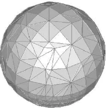
Figure 2.2: Approximation of a sphere using triangular facets
The methods mentioned up to this point are applicable to high frequency problems. By high-frequency phenomena, it is meant that fields are being con-sidered in a system where the properties of the medium and scatterer size param-eters vary little over an interval on the order of a wavelength. In other words, what restricts the application of a high-frequency method is the fact that the size of a scatterer must be large in terms of the wavelength at the given frequency. Thus, the above mentioned constraint is already satisfied. The computer pro-gram assumes the value of 200λ2 for the area of a facet. In other words, each facet is assumed to be equilateral triangles of edge length no more than 10λ. This length
is small enough for the high frequency approach. Smaller values may also be used to obtain more accurate results but of course with the expense of longer run times.
In evaluating the PO integral numerically, the contributions from each facet is calculated separately. Thus, the facets should be small enough so that the normal vector of a facet can safely be assumed to be constant through the entire surface of it.
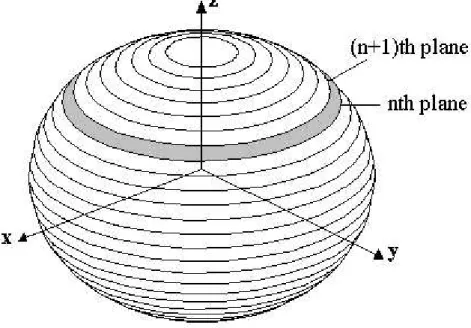
The target surface is first described by its boundary values. Using this in-formation, the target is split into a number of planes along z-axis as shown in Figure 2.3. Number of planes used in describing the target surface is unknown
Figure 2.3: Contouring the target by splitting along z-axis
and should be determined. Note that these planes may not be equally spaced along z axis. If the number of points on each plane is known, then the problem is to find out the z components of the planes (see Figure 2.4). To determine the relation between the number of points to be taken on each plane and the total surface area, the surface area between two consequent planes is calculated
(the shaded area in Figure 2.3). Then, number of triangles that should cover the region between nth and (n + 1)th planes is found by dividing the area to
λ2
200, which is the predefined value for the area of each triangle. Note that the
number of triangles is twice the number of points taken on each contour unless one of the planes is not composed of only a single point. Once, the number of triangles needed to cover the surface area between two consequent planes is determined, call it T, then T2 equally spaced points are chosen on each contour (number of points to be taken is the same for each contour). If T, the number of triangles needed, is an odd number, then T
2 is rounded to the nearest bigger
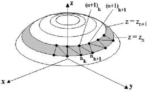
integer. The cartesian coordinates for the vertices of the triangles are determined but the parameters that must be determined for each triangle are its vector area and the coordinates of its midpoint. These parameters are determined using the coordinates of the vertices. As depicted in Figure 2.4, kth and (k + 1)th points
Figure 2.4: Triangular facets on the surface
on plane n and kth point on plane n + 1 form a triangle. Vertices of the next
triangle are kth and (k + 1)th points on plane n + 1 and (k + 1)th point on plane
n. This process is repeated starting from the first points of both planes until last points are reached (see Figure 2.4). When the region between the planes n
and n + 1 is completely filled, this process is repeated for the region between the planes n + 1 and n + 2 and so on. Calculating the area and midpoint of each facet for a sphere of radius R is presented next.
Spherical coordinates of a point on plane n and n + 1 are (R, θn, φn) and
(R, θn+1, φn+1) respectively. θn and θn+1 can be expressed as
θn = arccos zn R (2.13) θn+1 = arccos zn+1 R (2.14)
The surface area between these two planes is given by
An,n+1= Z θn θn+1 Z 2π 0 sin θr2dφdθ (2.15)
and evaluating (2.15) gives
An,n+1 = 2πr2(cos θn+1− cos θn) (2.16)
Using (2.13) and (2.14) in (2.16), the surface area between planes n and n + 1 is found to be An,n+1 = 2πr2( zn+1− zn R ) (2.17) then, T = An,n+1λ2 200 = (400πR 2 λ2 )( zn+1− zn R ) (2.18)
If N (the number points to be taken on each plane) is known, using the fact T = 2N and (2.18), zn+1 can be written in terms of zn as
zn+1 = zn+
λ2N
200πR (2.19)
Starting from z = 0, z component of every plane can be found using (2.19). This equation is applied until zn+1 exceeds R. Once z values are found, referring to
and plane n + 1 are found using the coordinates of vertices. The coordinates for midpoints of all facets (Xi, Yi, Zi) can be written as:
X2k−1 = x(n+1)k+ x(n+1)k+1+ xnk+1 3 X2k = x(n+1)k+ xnk+ xnk+1 3 Y2k−1 = y(n+1)k + y(n+1)k+1+ ynk+1 3 Y2k = y(n+1)k + ynk+ ynk+1 3 Z2k−1 = z(n+1)k+ z(n+1)k+1+ znk+1 3 Z2k = z(n+1)k+ znk+ znk+1 3 f or k = 1 : N (2.20)
where N is the number of points per plane. Referring Figure 2.5, area of a facet can be written as:
Area = 1 2|
−→
AB ×−→AC| = 1
2ab sin α (2.21)
Figure 2.5: Triangular facet on the surface
Normal vector ˆn is a unit vector with its tip at the midpoint of the triangle. Then ˆn can be expressed as the cross product of the vectors −→AB and−→AC. These vectors are
−→
−→
AC = (xC − xA)ˆx + (yC− yA)ˆy + (zC− zA)ˆz (2.23)
Once −→AB and−→AC are found, ˆn can directly be found by ˆ
n = −→ AB ×−→AC
|−→AB||−→AC| (2.24) To calculate the PO surface integral, ˆn and midpoint of the triangles given by (2.20) are stored for each triangle.
If a total of P triangles are used to cover the actual surface, the computer program produces an output of P by 7 matrix, each row representing a triangle. In each row x, y, and z components of the midpoint is stored in the first three columns, where fourth column stands for the area of the triangle and the last three columns represent the unit vector ˆn.
2.3
Physical Optics Formulation
In the presence of a perfectly conducting surface, the total electromagnetic field of a source may be expressed as a superposition of the incident fields (Ei, Hi) and
the fields (Es, Hs) which are scattered by the surface. The scattered fields can
be expressed in terms of the radiation integrals over actual currents induced on the surface of the scatterer. Physical Optics method assumes that the induced surface currents on the scatterer surface are given by the geometrical optics currents over those portions of the surface directly illuminated by the incident field, and zero over the shadowed sections of the surface:
¯ JP O = 2ˆn × ¯Hi , illuminated region 0 , shadow region (2.25)
where ˆn denotes the outward unit normal vector on the surface. Once this induced current is calculated, it is used in a radiation integral to find the scattered field. Since radiation integral for the scattered field is calculated by employing a GO approximation for the currents induced on the surface, it can be concluded
that PO is a high frequency method, which implies that target is assumed to be electrically large.
If the source is at a great distance from the target, it will illuminate the target with an incident field which is essentially a plane wave. The incident electric field intensity is given by (with ejωt time dependence):
¯
Ei = (Eθiθˆi+ Ei
φφˆi)ejk ˆri·¯r (2.26)
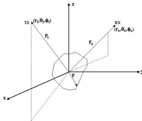
where (ri, θi, φi) are the spherical coordinates of the source and ( ˆri, ˆθi, ˆφi) are the
unit vectors. An arbitrary point on the target surface is assigned the coordinates (r, θ, φ). Note that such a point is the midpoint of a triangle and these coordinates are known after meshing process. Similarly, the observation point is assigned the coordinates (rs, θs, φs) and the unit vectors ( ˆrs, ˆθs, ˆφs). These parameters are
depicted in Figure 2.6.
The magnetic field intensity of the incident field is given by ¯ Hi = 1 ηˆk × ¯E i, = (Eφiθˆi− Eθiφˆi) ejkˆri·¯r η . (2.27)
For the scattered field, the vector potential is given by ¯ A = µ 4πrs e−jkrs Z Z ¯ Jejkˆrs·¯rds (2.28)
For a far-field observation point, the following approximation holds ¯ Es= −jω ¯A, = −2πrjωµ s e−jkrs Z Z ˆ n × ¯Hiejkˆrs·¯rds. (2.29) using (2.27) in (2.29) gives ¯ Es= e −jkrs rs (Eφiθˆi− Eθiφˆi) × ( j λ) Z Z ˆ nejk(ˆri+ˆrs)·¯rds. (2.30)
a new vector equal to the second term on the right hand side of (2.30) is defined: ¯ S = (j λ) Z Z ˆ nejk(ˆri+ˆrs)·¯rds. (2.31)
the scattered field may also be represented by: ¯
Es = (Eθsθˆs+ Eφsφˆs)
e−jkrs
rs
(2.32)
from (2.30), (2.31), (2.32) and the vector identity ¯ A · ( ¯B × ¯C) = ( ¯A × ¯B) · ¯C it is found that ¯ Es θ = (Eθiφˆi× ˆθs+ Eφiθˆs× ˆθi) · ¯S ¯ Es φ= (Eθiφˆi× ˆφs+ Eφiφˆs× ˆθi) · ¯S. (2.33)
equations in (2.33) can be cast into a single matrix equation: Es θ Es φ = ( ˆφi× ˆθs) · ¯S ( ˆθs× ˆθi) · ¯S ( ˆφi× ˆφs) · ¯S ( ˆφs× ˆθi) · ¯S Ei θ Ei φ (2.34)
The 2 × 2 matrix in (2.34) is the scattering matrix, which relates ¯Es to ¯Ei
component by component. To find the elements of the scattering matrix, (2.31) must be solved for given ˆri, ˆrs, ˆr and ˆn. These quantities are available after
the meshing process is performed as mentioned in Section 2.2 and are shown in Figures 2.5 and 2.6. Since (2.31) is a surface integral, ¯S can be found by superposing the contributions from each triangle. For a single facet as shown in Figure 2.5, this quantity is:
¯ St = ( j λ)ˆnte jk(ˆri+ˆrs)·¯rt4s t for t = 1 : K (2.35)
where K is the total number of illuminated facets on the surface, and 4st is the
area of the tth facet. Then, ¯S can be written as
¯ S = (j λ) X t ˆ ntejk( ˆri+ˆrs)·¯rt4st. (2.36)
Once, ¯S is computed, the scattering matrix can be found for given directions of incident and scattered fields. Note that, only the illuminated facets make con-tribution to the summation in (2.36). To find out whether a facet is illuminated or not, a new quantity It is defined. The facet is
illuminated if It > 0
shadowed if It < 0
(2.37)
where
It= ˆnt· ˆri (2.38)
Figures 2.8 through 2.23 display the numerical results for scattering by several different targets.
The scattering matrix for such targets, which have axial symmetry with re-spect to z-axis, closed form expressions for (2.31) can be derived [7]. The results presented here closely agree with the ones depending on the closed form solutions in [7]. This agreement does not mean that these results agree with the exact scat-tering data but shows that the computer program generates the correct Physical Optics data.
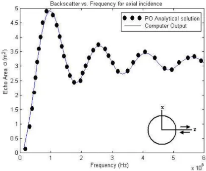
Scattering data for a sphere of radius 1 m are presented in Figures 2.8 through 2.11. Figure 2.8, shows the curve of backscatterer echo area versus frequency for axial incidence. It is observed that echo area approaches to πa2, which is the
geometric cross section of the target, with increasing frequency. The oscillatory
Figure 2.7: GO reflected and PO diffracted waves
Figure 2.8: Scattering data for a sphere with a radius of one meter (Backscatterer vs. frequency )
behavior of the RCS pattern is due to the interaction of GO reflected field and PO diffracted field contributions. GO reflected ray corresponds to the station-ary phase contribution and the PO diffracted fields correspond to the end-point contribution in the asymptotic integration of PO. PO diffracted field travels an
additional path length equal to the sphere diameter (see Figure 2.7), thus the peaks occur when this path difference is an integer multiple of λ (4f=c/path difference, where c is the speed of light).
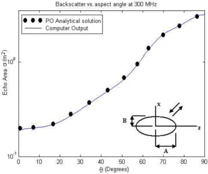
Figure 2.9 shows the variation of RCS as a function of aspect angle for the same sphere. The pattern in Figure 2.9 is a nice tool to find out whether the target is meshed adequately or not. Since the target is perfectly symmetric with respect to the origin, backscatterer echo area should be the same for every value of θ. Scattering data for different number of meshes are depicted in the Figure. The pattern becomes nearly constant as the number of meshes used to cover the surface of the target is increased. The result is satisfactory when 3120 meshes are used.
Figure 2.9: Scattering data for a sphere with a radius of one meter (Backscatterer vs. Aspect angle at 300MHz )
Figure 2.10: σθθ for a sphere with a radius of one meter (Bistatic scattering at
300MHz)
Figure 2.11: σφφ for a sphere with a radius of one meter (Bistatic scattering at
Figures 2.10 and 2.11 show E-plane bistatic scattering and H-plane bistatic scattering (σθθ and σφφ, respectively) for a sphere of radius 1m. RCS is the
largest for both polarizations for θ = 180o (forward scattering).
Figure 2.12: Scattering data for a prolate spheroid with A=1m and B=0.5m (Backscatterer vs. frequency)
Scattering data for a prolate spheroid of radius 1m are presented in Figures 2.12 through 2.15. Figure 2.12 shows the curve of backscatterer echo area versus frequency for axial incidence. Radius of curvature of the spheroid at the point on the axial direction can be calculated through the use of following formula [1]:
a(u) = −(c
2cos2u + d2sin2u)3/2
cd . (2.39)
where u is the angle that the ray from the origin to the reflection point makes with the z-axis and c and d are two principal radius of curvatures of the ellipse on the x-z plane (represented by A and B in Figure 2.12). With c = 0.5m, d = 1m and u = 0o, radius of curvature is found to be 0.25m. Thus in the
limit k −→ ∞, echo area approaches to the geometric cross-section of the sphere of radius 0.25m, which is 0.196 (see Figure 2.12). Occurrence of peaks in the 0 − 600MHz interval during the oscillation is the same as the one for the sphere
Figure 2.13: Scattering data for a prolate spheroid with A=1m and B=0.5m (Backscatterer vs. aspect angle at 300 MHz)
Figure 2.14: σθθ for a prolate spheroid with A=1m and B=0.5m (Bistatic
Figure 2.15: σφφ for a prolate spheroid with A=1m and B=0.5m (Bistatic
scat-tering at 300MHz)
Figure 2.16: Scattering data for an oblate spheroid with A=0.5m and B=1m (Backscatterer vs. frequency)
Figure 2.17: Scattering data for a prolate spheroid with A=1m and B=0.5m (Backscatterer vs. aspect angle at 300 MHz)
because phase difference between the diffracted and reflected fields is the same for two cases (2 m in both cases).
Figure 2.13 shows the variation of RCS as a function of aspect angle for the prolate spheroid. Echo area increases as θ increases because the area that intercepts the incoming wave increases as θ increases. E-plane bistatic scattering (σθθ) and H-plane bistatic scattering (σφφ) for the prolate spheroid are depicted
in Figures 2.14 and 2.15. Figure 2.16 shows the curve of backscatterer echo area versus frequency for axial incidence for an oblate spheroid. Using (2.39) with c = 1m, d = 0.5m and u = 0o, radius of curvature of the spheroid at the point
on the axial direction is 2m. Thus, in the limit k −→ ∞, echo area approaches to the geometric cross-section of the sphere of radius 2m, which is 12.56m2 (see
Figure 2.16). Number of peaks in the 0 − 600MHz interval is less than the one for sphere and prolate spheroid. This is due to the fact that the diffracted field this time travels an additional distance of 1 m and 4f = c/1.
Figure 2.18: σθθ for a oblate spheroid with A=0.5m and B=1m (Bistatic
scat-tering at 300MHz)
Figure 2.19: σφφ for a oblate spheroid with A=0.5m and B=1m (Bistatic
It is also observed from Figures 2.8, 2.12 and 2.16 that
4foblatesphereoid > 4fprolatesphereoid > 4fsphere (2.40)
which is consistent with the calculations. E-plane bistatic scattering (σθθ) and
H-plane bistatic scattering (σφφ) for the prolate spheroid are depicted in Figures
2.18 and 2.19.
Figures 2.20 through 2.23 show the scattering data for an ogive and a cone. Note that, these two shapes have edges, which makes large contributions to the scattered field especially around the GO boundaries. The results presented here only contains the PO component of the scattered field and compared with the PO analytical solutions. These result do not contain any information on the edge-scattered fields, meaning that for these two shapes, the difference between the actual scattering data and the computer output may be larger compared to the previous simulations.
Chapter 3
Equivalent Edge Currents
Method of equivalent edge currents (EEC) is a powerful technique in the analysis of scattering. Any finite current distribution yields a finite result for the far-zone diffracted field when that distribution is summed in a radiation integral. Thus, the invalidity of the GTD diffraction at the caustics can be avoided by the use of a proper current distribution on the edge. In addition, the method also allows the calculation of diffracted fields in the scattering directions that are away from the cone of diffracted fields. The concept of equivalent edge currents is discussed in [1], [6] and [8] in detail.
Method of equivalent edge currents depends on finding currents that would, when integrated along the edge, give a known value of radiated field at the obser-vation point. In other words, EEC method yields the result that already appears to be correct at the specified observation point. GTD equivalent currents asymp-totically yield GTD field at the observation point. It is also possible to derive the equivalent edge currents from the surface current density induced by the incident field. This approach is first introduced by Millar and developed by Mitzner and Michaeli[9]. Later, there has been some improvements and modifications in this
surface-current-based equivalent edge currents [11]. The equations presented in [11] are used in this work.
3.1
Formulation of Equivalent Edge Currents
Let us consider the scattering from flat plates. The scattering configuration is shown in Figure 3.1. To calculate the equivalent currents along the edge of an arbitrary flat plate with an arbitrary geometry, the edge is approximated using half planes.
Figure 3.1: Scattering configuration
The vector ˆrsdenotes the position vector of an arbitrary surface element and
ˆ
re is the position vector of an edge element. Since, calculations are done for
far-field observation points, the unit vectors ˆr, ˆs and ˆR are approximated to be equal to each other. In the PTD approach, total scattered field is divided into two components; the PO field and the fringe wave (FW) field:
¯
These fields are generated by the physical optics and fringe wave surface current densities ( ¯JP O and ¯JF W respectively). In other words, the induced current can
be decomposed into PO and non-uniform (fringe) components, so that ¯
Jtot = ¯JP O + ¯JF W (3.2) Just like FW field, being a correcting contribution that must be added to the PO field to obtain the exact field, fringe wave current is a correcting contribution to the PO current to obtain the total current.
The first term on the right hand side of (3.1) is the PO surface integral and is calculated using the procedure explained in Chapter 2. This chapter is devoted to the calculation of the edge-diffracted field, the second term on the right hand side of (3.1).
For a far-field observation point, the field caused by an induced current of ¯J on a surface S is given by ¯ Es(r) = jkζ Z Z S ˆ R × ( ˆR × ¯J)e−jkR 4πRds 0 (3.3)
This surface integral may be evaluated over the near-edge points because con-tribution from the rest of the surface is negligible. If this region is denoted as Sedge, total scattered field can asymptotically be expressed as
¯ Es(r) ∼ ¯EsP O+ jkζ Z Z Sedge ˆ R × ( ˆR × ¯JF W)e −jkR 4πR ds 0 (3.4)
and EF W,the scattered field due to ¯JF W, is
¯ EF W ∼ jkζ Z Z Se ˆ R × ( ˆR × ¯J)e −jkR 4πR ds 0 (3.5)
To describe the scattered field in terms of edge currents, the equation in (3.5) is expressed in terms of new integration variables ` and u (see Figure 3.2). Here, ` is the arc length along the edge measured starting from an arbitrary point. The total length of the edge is L. The unit vector ˆu might be different
Figure 3.2: Integration variables l and u.
for different values of ` and points inwards away from the edge. For a far-field observation point, R appearing in the phase term in (3.5) can be approximated by s − ˆs · (¯rs − ¯re) = s − ˆs · ˆuu taking the phase reference as the origin. ˆR
can be approximated by ˆs and the distance appearing in the denominator can be approximated by s. It is clear that, the integration limits for the variable ` is 0 and L. For u, the lower limit is 0 and specification of the upper limit is not necessary since the only contribution to the integral is from the edge points where u = 0. Incremental area ds0 on the scatterer surface is equal to |ˆu × ˆt|dudl.
Using these approximations in (3.5), diffracted field caused by the fringe currents on the scatterer is:
¯ EF W ∼ jkζ Z Z Se ˆ s × (ˆs × ¯JF W)e −jk(s−ˆs·ˆuu) 4πs ds 0, = jkζ Z L 0 |ˆu × ˆt| e−jks 4πs s × [ˆs ׈ Z 0 ¯ JF Wejkˆs·ˆuu)du]dl. (3.6)
This expression states that [8] the incremental diffracted field associated with the end point at the position ¯re is the endpoint contribution to the field generated by
the surface currents density ¯JF W on an incremental strip starting at that edge
The diffracted field generated by an incremental element on the edge can be assumed to be generated by line currents induced on the edge. This electric and magnetic line currents are located at position ˆre and points the same direction
as ˆt. The field generated by these currents is given by ¯ E = jk Z L 0 e−jks 4πs [ζ ˆs × (ˆs × ˆt)I + ˆs × ˆtM]dl (3.7) Expressions for I and M (will be denoted by IF W and MF W from this point on)
are found by equating (3.7) to (3.6):
IF W = | ˆu × ˆt | | ˆs × ˆt |2s · (ˆt× ˆs) ׈ Z 0 ¯ JF Wejkˆs·ˆuudu (3.8) MF W = ζ | ˆu × ˆt | | ˆs × ˆt |2ˆt · ˆs × Z 0 ¯ JF Wejkˆs·ˆuudu (3.9) The term ¯JF W appearing in these equations is the fringe wave surface current
density and is integrated along the direction ˆu to yield the expressions for fringe wave electric and magnetic currents on the edge. IF W and MF W are then used
in (3.7) to give the total fringe wave diffracted field, EF W. Currents expressed
by (3.8) and (3.9) are called the Physical Theory of Diffraction-Equivalent Edge Currents (PTDEEC). A similar derivation could be written for the PO current (POEEC) [10], however, PO integral is left as a surface integral in this work. PTDEEC are then used as an improvement to PO for edged bodies.
Since, the actual edge geometry is modelled by half planes, it is the half plane surface current density that is integrated along ˆu to give IF W and MF W
in (3.8) and (3.9). The actual edge is modelled using half-planes as depicted in Figure 3.3. The incremental diffracted field caused by each segment (the length dl) on the edge of the actual scatterer is then found using (3.7) Expressions for IF W and MF W depend on the characteristics of the local configuration, i.e. the
tangential components of the incident electric and magnetic fields, the directions of incidence and observation, and on the direction of ˆu (at non-stationary points only).
Figure 3.3: Integration variables l and u.
3.2
PTD-EEC
As mentioned in the previous section, the only contribution to the incremental diffracted field is from the edge. This approximation makes possible to use only the lower limit in (3.8) and (3.9).
For the FW surface current, it is found that the end-point contribution is identical to the result of an explicit integration along the incremental strip start-ing at the edge and extendstart-ing to infinity [8]. Thus, FW parts of the equivalent edge currents, using (3.8) and (3.9), can be expressed as
IF W = | ˆu × ˆt | | ˆs × ˆt |2s · (ˆt× ˆs) ׈ Z ∞ 0 ¯ JF Wejkˆs·ˆuudu (3.10) MF W = ζ | ˆu × ˆt | | ˆs × ˆt |2t · ˆs ׈ Z ∞ 0 ¯ JF Wejkˆs·ˆuudu (3.11) Fringe wave component of the scattered field is found using (3.10) and (3.11) in (3.7). For the configuration depicted in Figure 3.4, total surface current density
is found by applying the boundary condition (using cylindrical coordinates) ¯
J(ρ, z) = ˆy × ( ¯H(ρ, 0, z) − ¯H(ρ, 2π, z)) (3.12)
The exact solution to the problem in Figure 3.4 is found by Sommerfeld and can be expressed as (from Breinbjerg [8]):
Ez = ¯E0i · ˆze jπ/4 √ π [e jk sin θiρ cos(φ−φi) F (−p2k sin θiρ cos(φ−φi 2 ))
−ejk sin θiρ cos(φ+φi)
F (−p2k sin θiρ cos(φ+φi 2 ))]ejkz cos θ i (3.13) Hz = ¯H0i· ˆze jπ/4 √ π [e jk sin θiρ cos(φ−φi) F (−p2k sin θiρ cos(φ−φi 2 )) +ejk sin θiρ cos(φ+φi) F (−p2k sin θiρ cos(φ+φi 2 ))]e jkz cos θi (3.14)
where, F is the Fresnel function and is given by
F (x) = Z ∞
0
e−jt2dt (3.15)
Using (3.12) and (3.13) with ρ = x, the resulting expressions for the half-plane FW surface current density can be expressed as [8]:
JxF W(x, z) = − ¯H0i· ˆz4e jπ/4 √ π F ( √ 2kx sin θicosφ i 2) .ejk(x sin θicos φi+z cos θi)
(3.16) JzF W(x, z) = −(1 ζE¯ i 0 · ˆz sin φi sin θi + ¯H i 0· ˆz cos θicos φi sin θi ) . 4e jπ/4 π12 F (√2kx sin θicosφ i 2)e
jk(x sin θicos φi+z cos θi)
+ (1 ζE¯ i 0 · ˆz sin φi 2 + ¯H i 0· ˆz cos φi 2 cos θ i) . 4e −jπ/4 √ π 1 sin θi√2kx sin θie −jk(x sin θi−z cos θi) (3.17)
Figure 3.4: Half plane illuminated by a plane wave
An asymptotic expression for the FW current is necessary to find the equiva-lent currents (see (3.10) and (3.11)) since the vector ˆu extends to infinity. When the argument of F is large, it can be approximated as
lim
x→∞F (x) =
e−jx2
j2x (3.18)
Using (3.18) in (3.16) and (3.17), x and z components of the FW current density are found to be Jxf w= − ¯H0i· ˆz2e −jπ/4 √ π e−jk(x sin θi−z cos θi) √ 2kx sin θicosφi 2 Jzf w= ¯H0i· ˆz 2e−jπ/4 √ π cos θi sin θi e−jk(x sin θi−z cos θi) √ 2kx sin θicosφi 2 (3.19)
¯ Jf w = −ˆu ¯H0i · ˆz2e −jπ/4 √ π e−jk ˆu·¯r √ 2kx sin θicosφi 2 sin θi (3.20) where ˆ u = ˆx sin θi − ˆz cos θi (3.21) This means that the strip that ¯Jf w is integrated along lies at the intersection of
the Keller cone with the half-plane and points to the direction of ˆn as shown in Figure 3.4. Choosing the direction along which the integral is evaluated to be the intersection of the Keller cone with the surface is the origin of the development of the EEC equations used in this work. These equations, introduced by Michaeli [11], will be discussed next.
3.3
PTD-EEC for a Wedge
Figure 3.5: Wedge geometry
To apply the EEC method to a wedge, the configuration is replaced by the one in Figure 3.5. The equations for the half-plane directly apply to face-1. For
face 2, x remains the same and y points opposite to its current direction. Thus, z also changes its direction to -z. This means that, the equations for EEC’s related to face 1 can be used to find the EEC’s related to face 2 with the following change of variables; z → −z, β → π − β, β0 → π − β0, φ → Nπ − φ, φ0 → Nπ − φ0.
Then, equivalent electric and magnetic edge currents take the form: ¯
I = (I1− I2)ˆz
¯
M = (M1− M2)ˆz
(3.22)
where I1, M1 are related to the surface current density on face 1 and I2, M2 are
related to the surface current density on face 2. As mentioned in Section 3.1, I1
and M1 can be split into its PO and FW components.
¯
I1f = I1− I1P O
¯
M1f = M1− M1P O
(3.23)
where (from Michaeli[11])
I1P O = 2jU (π − φ 0) k sin β0(cos φ0+ µ)[ sin φ0 Z sin β0z · ¯ˆ E i 0
− (cot β0cos φ0 + cot β cos φ)ˆz · ¯Hi
0] (3.24)
M1P O = −2jZ sin φU(π − φ
0)
k sin β sin β0(cosφ0+ µ)z · ¯ˆ H i 0 (3.25) I1 = 2j k sin β0 1 N cosφN0 − cos(π−αN ) · [ sinφN0 Z sin β0z · ¯ˆ E i 0 +sin π−α N sin α · (µ cot β 0− cot β cos φ)ˆz · ¯Hi 0] − 2j cot β 0 kN sin β0z · ¯ˆ H i 0 (3.26) M1 = 2jZ sin φ k sin β0sin β 1 N sinπ−αN csc α cos π−α N − cos φ0 N · ¯H0i (3.27) where ¯Ei
0 and ¯H0i are the incident electric and magnetic field vectors at the point
function and α = arccos µ = −j ln(µ + jp1 − µ2), (3.28) µ = cos γ − cos 2β0 sin2β0 = 1 − 2 sin2 γ2 sin2β0 (3.29)
cos γ = ˆu · ˆs = sin β0sin β cos φ + cos β0cos β (3.30)
Choosing the direction of ˆu as the direction of the grazing diffracted ray reduces the number of singular directions. These expressions are singular for degenerate cases such as glancing incidence (φ0 = π) or edge-on incidence (β → 0 or β → π).
The latter one is in fact is insignificant because the diverging term disappears when substituted in the radiation integral (see (3.7)).
Based on the change of variables listed before for face 2, total equivalent edge currents can be expressed as
If = I1f − I2f (3.31)
Mf = M1f − M2f (3.32) Using equations (3.23)-(3.28), final expressions for If and Mf for a half-plane
(N=2, Figure 3.5) are If = Eti 2jY k sin2β0 √ 2 sinφ20 cos φ0+ µ[p1 − µ − √ 2 cosφ 0 2] + Hi t 2j k sin β0 1 cos φ0+ µ[cot β
0cos φ0+ cot β cos φ
+ √2 cosφ0 2
µ cot β0− cot β cos φ
√ 1 − µ ] (3.33) Mf = Hti 2jZ sin φ k sin β sin β0 1 cos φ0+ µ[1 − √ 2 cos φ20 √ 1 − µ ] (3.34)
where Y = Z−1, Ei
t = ˆz · ¯E0i, Hti = ˆz · ¯H0i. For the half-plane case, the only
singularity occurs when ˆs = ˆs0 = ˆu or β = β0, φ0 = π, φ = 0 for face 1. Similarly,
a singularity occurs for face 2 when the observation direction is the continuation of the incident ray, grazing face 2 from the outside [11].
For monostatic RCS calculations, expressions for backscattering are derived using (3.23) through (3.28). Having obtained the expressions for I1f and M1f, the expressions for I2f and M2f are found directly by the change of variables. In the backscattering case, β = π − β0, φ = φ0 and (3.28) simplifies to (3.35) and (3.36)
for face 1 and face 2 respectively.
α1 = arccos µ1 = arccos(cos φ − 2 cot2β) (3.35)
α2 = arccos µ2 = arccos(cos(N π − φ) − 2 cot2β) (3.36)
Fringe current densities for backscattering are given by (3.37) and (3.38). (3.37) and (3.38) with (3.35) and (3.36) derived for backscattering do not involve any singularities except the degenerate cases just mentioned and are used in the computer program for the backscattering calculations.
If = −2jY k sin2β[ sin φU (π − φ) cos φ + µ1 + 1 N sin φ N cos π−α1 N − cos φ N ]ˆz · ¯E0i + 2j sin π−α1 N N k sin β sin α1
µ1cot β0− cot β cos φ
cosNφ − cosπ−α1 N ˆ z · ¯H0i − { −2jY k sin2β[ sin(N π − φ)U(π − Nπ + φ) cos(N π − φ) + µ2 + 1 N sinN π−φN cosπ−α2 N − cosN π−φN ](−ˆz · ¯E0i) + 2j sin π−α2 N N k sin β sin α2
cot β cos(N π − φ) − µ2cot β0
cosN π−φN − cosπ−α2
N
(−ˆz · ¯H0i)}
Mf = 2jZ sin φ k sin2β [ U (π − φ) cos φ + µ1 − 1 N sinπ−α 1 N csc α1 cos Nφ − cosπ−α1 N ]ˆz · ¯H0i − {2jZ sin(N π − φ) k sin2β [ U (π − Nπ + φ) cos(N π − φ) + µ2 − 1 N sinπ−α 2 N csc α2 cosN π−φN − cosπ−α2 N ]}(−ˆz · ¯H0i) (3.38)
3.4
Numerical Results
In this section, scattering data for several configurations are calculated. The results are compared with the results that are currently available in the literature. Discrepancies of the method used in this work are also mentioned.
The square plate configuration depicted in Figure 3.6 will be presented first. Expressions for If and Mf for this configuration are found using (3.33) with
β0 = φ0 = π 2 and N = 2: If = t · ¯Ei2 √ 2jY sinπ 4 kµ [p1 − µ − √ 2 cosπ 4] + t · ¯Hi2j kµ[cot β cos φ − √
2 cosπ4 cot β cos φ √ 1 − µ ] (3.39) Mf = t · ¯Hi2jZ sin φ k sin βµ [1 − √ 2 cosπ 4 √ 1 − µ ] (3.40) where µ = sin β cos φ (3.41)
and ˆt is the direction of the equivalent currents. σφφ vs. θ for the square plate
configuration is depicted in Figure 3.7 with the MOM result from Breinbjerg [8]. The deep nulls throughout the pattern are caused by the destructive interference of the fields caused by two orthogonal edges. Furthermore, as mentioned earlier only the first order diffractions are calculated in this work. Since the FW current is assumed to be travelling to infinity in accordance with the half plane geometry,
Figure 3.6: Square plate configuration
diffraction caused by the same current at another edge is neglected (second-order diffraction). This effect can also be reduced by using a larger plate.
A similar configuration is depicted in Figure 3.8. Bistatic scattering from the edge of a disc, obtained by using (3.39) and (3.40), is presented in Figure 3.8. A φi polarized wave is normally incident on a disc and the plane of observation is
the y − z plane. Three different disc sizes, ka = 5, 10 and 15 are investigated.
It is observed that the agreement between the results presented in Figure 3.8 and the exact results, from Breinbjerg [8], improves with increasing disc radius. The edge interaction effects decrease as the disc size becomes larger. When the disc size is small, the FW surface current possess sufficient strength to cause diffraction at the edge point of interest after traversing the disc. This effect is decreased by increasing the radius of the disc.
The edge-diffracted field is added to the surface-diffracted field to obtain the total scattered field at the observation point. The computer program computes
Figure 3.7: RCS σφφ of a square plate of area 36λ2
the PO surface integral for this purpose. Total scattered field can be written as: ¯
Etot = ¯EP T DEEC + ¯EP O (3.42)
Scattering from a cylinder of length l = 12.45/k and base radius a = 2.16/k is calculated using (3.42). The configuration and scattering data are depicted in Figures 3.9 and 3.10. In Figure 3.10, RCS obtained using only the PO component and RCS obtained using the total scattered field are plotted separately to observe the effect of edge diffraction. The experimental results (from Shaeffer [12]) are also plotted in Figure 3.10.
The surface of the cylinder is approximated with 950 triangles. Experimental results are normalized to σ0 = 0.0052, and the measurement frequency is 2.6GHz.
Figure 3.9: Cylinder configuration. Backscattered field vs. θ is computed at φi = φs = π/2
It should be noted that, whole edge contributes to the edge-scattered field for the top face of the cylinder whereas only the half of the edge contributes to the scattered field for the bottom face for the same observation angle. Equiva-lent currents are assumed to exist at an edge segment if only it is illuminated. Otherwise no FW currents are induced at the edge point. The pattern depicted in Figure 3.10 shows a good agreement with the experimental results. Results of the computer program would be more accurate if the dimensions of the cylinder were electrically larger.
Chapter 4
SCATTERING BY THIN
WIRES
This chapter is devoted to the study of scattering mechanisms that includes thin wires. As indicated in Chapter 1, scattering by a thin wire cannot be calculated using the techniques mentioned previously in this report. Travelling wave energy plays a significant role in the overall scattered field on a straight wire. This was demonstrated by Hong [4]. It was suggested that the source of backscattering from a thin wire is a travelling wave, launched at the near end and then reflected at the far end. Thin wire scattering in this work is based on the method described in [4] and [5].
4.1
Scattering Mechanisms
Consider a wire of length L and radius a that is centered on the z-axis as shown in Figure 4.1. Expressions for each scattering mechanism on a straight wire are cast in the form of four basic wave concepts: diffraction, attachment, launch and reflection. These scattering mechanisms are also shown in Figure 4.1.
Figure 4.1: Geometry of a straight wire and scattering paths
When the incident wave reaches to either end of the wire, the incident field is diffracted by the tip of the wire and a travelling wave is is simultaneously attached along the wire. When this travelling wave reaches to the other end of the wire, a portion of its energy is diffracted and the remaining energy is reflected back forming a secondary travelling wave. This process goes on until the guided wave completely fades away as shown in Figure 4.1. Based on this process, Ufimtsev’s [13] representation of the backscattered field is [4]:
¯
E = ˆθ−e
jkr
kr
2jS(θ)
where γ = 1.781 is Euler’s constant and S(θ) = −{sin4 θ 2ln( j γka sin2(θ/2))} + {ej2kL cos θcos4 θ 2ln( j γka cos2(θ/2)) − ejkL(1+cos θ)cos4 θ 2ln( j γka cos(θ/2))2Ψ+ + ejkL(1+cos θ)sin4 θ 2ln( j γka sin(θ/2))2Ψ− + ej2kLcos θ ln( j γka)(Ψ+) 2 } + { ∞ X n=0 ej2nkLΨ2n[(Ψ)2(Ψ+)2ej4kL + (Ψ−)2ejkL2(1+cos θ)
− 2Ψ+Ψ−ΨejkL(3+cos θ)] cos θ ln(
j γka)}
(4.2)
The functions Ψ and Ψ∓ satisfy the Volterra equation of the first kind and represented in the form
Ψ = jπ − 2 ln(γka) ln(γkj2kL2a2) − E(2kL)e−j2kL (4.3) Ψ∓ = jπ − ln(γ 2q ∓) ln(γkj2kL2a2) − E( 2kLq∓ k2a2 )e −j2q∓k2a2kL (4.4) q∓= (ka) 2 2 (1 + cos θ) (4.5) E(x) = Z x ∞ ejt t dt (4.6)
Each term appearing in (4.2) corresponds to one of the specific ray paths shown in Figure 4.1. For a straight wire as depicted in Figure 4.1, all of these terms are included into the total scattered field. However, when the wire is attached on a body, some of them should be neglected.
To examine the results as a function of angle, scattering from a perfectly conducting straight wire of length L = 19.5 in with radius of a = 0.0118 in at 10 GHz is calculated using (4.1) through (4.6). The output of the computer program perfectly agrees with the MOM result [5] as seen from Figure 4.2.
Figure 4.2: Backscattered field from a 19.5 in long perfectly conducting wire of radius 0.0118 in, MOM and program output
4.2
Wire-Attached Bodies
Consider the configuration depicted in Figure 4.3, in which the wire is attached to a cylinder at one of its endpoints. As mentioned in the previous section, each term in (4.2) corresponds to a different path. All of the terms are included to calculate scattering from an isolated wire. For the configuration in Figure 4.3 however, the terms corresponding to the diffraction from endpoint B and the terms corresponding to the paths that include attachment from endpoint B should be neglected.
Neglecting the above mentioned terms in S(θ), what remains is only the terms that correspond to the attachment and diffraction from endpoint A:
S(θ) = −{sin4 θ2ln( j γka sin2(θ/2))} + {ej2kLcos θ ln( j γka)(Ψ+) 2 } (4.7)
Figure 4.3: Wire-attached cylinder configuration lc = 12.45/k, l=5.53/k,
a=2.16/k
Scattering from the wire-cylinder configuration is calculated at 2.6 GHz using (4.7) instead of (4.2). The results are presented in Figure 4.4. The effect of the thin wire to the total backscattered field is noticeable.
Figure 4.4: RCS σθθ of the cylinder+wire structure shown in Figure 4.3
Note that the scattering pattern for the cylinder remains the same for θ > 140o. Because, the region where θ > 140 (see Figure 4.3) is shadowed by the
(tip of the wire+edge of the cylinder), but it is omitted in this work since its contribution to the total scattered field is weak.
Chapter 5
CONCLUSIONS
In this work, a computer program which uses the Physical Theory of Diffrac-tion (PTD) method to calculate the RCS of perfectly conducting targets with arbitrary shape including edges or linear parasitics is developed.
Since, high-frequency techniques are used in calculations, what restricts the application of this computer program is the fact that the size of the scatterer must be large in terms of the wavelength at the given frequency (e.g. ka> 10 for a sphere).
Physical Optics method is used to calculate the scattering from smooth sur-faces. The theory of PO overcomes the catastrophe of the infinities of flat and singly curved surfaces by approximating the induced surface fields and by inte-grating them to obtain the scattered field. PO surface integral must be evaluated numerically. It should be noted that if PO integral is approximated asymptot-ically using the method of stationary phase, then what is obtained is the GO reflected field that is associated with the stationary phase point. Additionally, asymptotic end-point contribution can be considered as the diffraction of the PO. The target surface is meshed to numerically evaluate the PO surface integral.
The accuracy of the PO method depends on the size of the meshes. Triangles with area= 0.005λ2 are used for meshing. This mesh size is appropriate both
in terms of accuracy and run-time of the program. PO theory also includes erroneous contribution due to abrupt discontinuities of current at the shadow boundaries of the surface. PO approximation is also expected to be inaccurate in the regions where the GO current does not produce the dominant scattering (e.g. deep shadow regions). Furthermore, fields in the PO approximation do not satisfy reciprocity except in the direction of specular reflection.
PO becomes more inaccurate if the target surface contains edges. PTD is used to overcome this discrepancy. GO current approximation is improved by includ-ing a correction (that is the FW current) in the PTD approach. FW component of the current includes the effects not accounted for in the GO approximation to the surface current. In fact, PTD is the superposition of the PO field (originat-ing from the smooth surface) and the field of the equivalent currents on the edge (edge-diffracted field). Method of EEC’s depends on finding the currents that would, when integrated along the edge, give a known value of radiated field.
When attached to a body, contribution of a thin wire to the total scattered field may be large so that its effect cannot be omitted. For this purpose, the program calculates the scattering by thin wires using a method that depends on diffraction, attachment, reflection and launch. All of the multiple travelling waves on the wire can be expressed in a closed form representation, in terms of simple asymptotic coefficients. These expressions yield excellent agreement with the moment method solution for an isolated thin wire (see Figure 4.2). Only the tip diffraction term is included for the body+wire structure.
To finalize, having demonstrated that the computer program gives correct data for a variety of target shapes presented in this report, we have confidence that the program will perform equally well with other targets.
Bibliography
[1] D. A. McNamara, C. W. I. Pistorius, J. A. G. Malherbe, Introduction to The Uniform Geometrical Theory of Diffraction, Artech House, Boston, 1990. [2] P. H. Pathak, Techniques for High Frequency Problems, Antenna Handbook
Volume I, Chapter 4, Van Nostrand Reinhold, New York, 1993.
[3] T. B. Hansen, “Corner Diffraction Coefficients for the quarter plate”, IEEE Transactions on Antennas Propagation, Vol. 39 , NO.7, pp.976-984, July 1991.
[4] S. Hong, S. L. Borison, and D. P. Ford, “Short-Pulse scattering by a long Wire”, IEEE Transactions on Antennas Propagation, Vol. AP-16, NO.3, pp.338-342, May 1968.
[5] H. T. Shamansky, A. K. Dominek, L. Peters, “Electromagnetic Scattering by a Straight Thin Wire”, IEEE Transactions on Antennas Propagation, Vol. 37, NO.8, pp.1019-1025, August 1989.
[6] E. F. Knott, J. F. Shaeffer, and M. T. Tuley, “Radar Cross Section“, Artech House, Inc., USA, 1985.
[7] J. H. Richmond, “A computer Program For Physical-Optics Scattering by Convex Conducting Targets“, Deputy For Surveillance and Control Systems Electronic Systems Division Air Force Systems Command United States Airforce, L. G. Hanscom Field, Bedford, Massachusets, May 1985.
[8] O. Breinbjerg, “Equivalent Edge Current Analysis Of Electromagnetic Scat-tering By Plane Structures”, PhD thesis, Electromagnetics Institute, Tech-nical University of Denmark, LD 83, March 1991
[9] A. Michaeli, “Equivalent Edge Currents for arbitrary aspects of observa-tion”, IEEE Transactions on Antennas Propagation, Vol.32, no.3, pp.252-258, March 1984
[10] T. Oguzer, A. Altintas, O. Merih Buyukdura, “On the Elimination of infini-ties in in the PO component of Equivalent Edge Currents”, Wave Motion, Vol.18, pp.1-10, 1993
[11] A. Michaeli, “Elimination of infinities in equivalent edge currents, part I:Fringe current components”, IEEE Transactions on Antennas Propaga-tion, Vol.34, no.7, pp.912-918, July 1986
[12] John F. Shaeffer, “EM Scattering From Bodies of Revolution with At-tached Wires”, IEEE Transactions on Antennas Propagation, Vol.AP-30, no.3, pp.426-431, May 1982
[13] P. Ya. Ufimtsev, “Diffraction of plane electromagnetic waves by a thin cylin-drical conductor”, Radio Eng. Electron Phys., vol. 7, pp. 241-249, 1962.