Parallel direct volume rendering of unstructured grids based on object-space decomposition

ш м ш 2^

ем

¿ΒΘΨ

^жщтх-іХі

7;:'і!:У:к.:тшш

У :^

PARALLEL DIRECT VOLUME RENDERING

OF UNSTRUCTURED GRIDS

BASED ON OBJECT-SPACE DECOMPOSITION

A THESIS

SUBMITTED TO THE DEPARTMENT OF COMPUTER ENGINEERING AND INFORMATION SCIENCE AND THE INSTITUTE OF ENGINEERING AND SCIENCE

OF BILKENT UNIVERSITY

IN PARTIAL FULFILLMENT OF THE REQUIREMENTS FOR THE DEGREE OF

MASTER OF SCIENCE

By

Ferit Fındık

October, 1997

T

■ F5é

I certify that I have read this thesis and that in my opin­ ion it is fully adequate, in scope and in quality, as a thesis for the degree of Master of Science.

Assoc. Prof. Cevdet Aykanat( Principal .Advisor)

I certify that I have read this thesis and that in my opin­ ion it is fully adequate, in scope and in quality, as a thesis for the degree of Master of Science.

I certify that I have read this thesis and that in my opin­ ion it is fully adequate, in scope and in quality, as a thesis for the degree of Master of Science-.

\ .. .

.Asst.'Profr-Ijgur Güdükbay

.Approved for the Institute of Engineering and Science;

________

Prof. Dr. M e h m e t ^

Ill

A B S T R A C T

PARALLEL DIRECT VOLUME RENDERING OF UNSTRUCTURED GRIDS

BASED ON OBJECT-SPACE DECOMPOSITION

Ferit Fındık

M.S. in Computer Engineering and Information Science Supervisor: Assoc. Prof. Cevdet .\ykanat

October, 1997

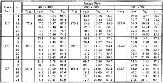
This work investigates object-space (OS) parallelization of an efficient ray­ casting based direct volume rendering algorithm (DVR) for unstructured grids on distributed-memory architectures. The key point for a successful paral­ lelization is to find an OS decomposition which maintains the OS coherency and computational load balance as much as possible. The OS decomposition problem is modeled as a graph partitioning (GP) problem with correct view- dependent node and edge weighting. As the parallel visualizations of the results of parallel engineering simulations are performed on the same machine. OS de­ composition, which is necessary for each visualization instance because of the changes in the computational structures of the successive parallel steps, con­ stitutes a typical case of the general remapping problem. .A GP-based model is proposed for the solution of the general remapping problem by constructing an augmented remapping graph. The remapping tool RM-MeTiS, developed by modifying and enhancing the original MeTiS package for partitioning the remapping graph, is successfully used in the proposed parallel DVR algorithm. -An effective view-independent cell-clustering scheme is introduced to induce more tractable contracted view-dependent remapping graphs for successive vi­ sualizations. .An efficient estimation scheme with high accuracy is proposed for view-dependent node and edge weighting of the remapping graph. Speedup values as high ¿is 22 are obtained on a Parsytec CC system with 24 processors in the visualization of benchmark volumetric datasets and the proposed DVR algorithm seems to be linearly scalable according to the experimental results.

Key words: Parallel Direct Volume Rendering, Unstructured Grids. Object-

IV

ÖZET

DÜZENSİZ IZGARALARIN

OBJE UZAYI BÖLÜNMESİNE DAYANAN PARALEL HACİM GÖRÜNTÜLENMESİ

Ferit Fındık

Bilgisayar ve Enformatik Mühendisliği, Yüksek Lisans Tez Yöneticisi: Doç. Dr. Cevdet .Aykauat

Ekim, 1997

Bu çalışma düzensiz ızgaraların ışın izlemeye dayanan verimli doğrudan hacim görüntüleme (DHG) algoritmasının çok-işlemcili dağıtık bellekli bilgisa­ yarlarda obje-uzayı (OU) paralelleştirilmesini araştırmaktadır. Başarılı bir paralelleştirmenin sırrı, OU benzerliğini koruyan ve mümkün olduğunca hesap- sal yük dengesini sağlayan OU bölümünü bulmaktır. OU bölümü problemi çizge bölünmesi (ÇB) problemi olarak bakış açısına bağımlı doğru düğüm ve kenar ağırlığı verilmesiyle modellendi. Paralel mühendislik sinıulasyon- larmın sonuçları aynı makiiıada paralel görüntülendiği için, ardışık paralel adımlarda oluşan hesapsal yapıdaki değişiklik. OU bölünmesini gerektirir ve bu bölünme genel yeniden eşleme problemine örnek teşkil eder. Genel \eniden eşleme probleminin çözümü için eklentili yeniden eşleme çizgesi oluşturarak, ÇB’ne dayalı bir model sunuldu. MeTiS ÇB aracını değiştirerek, yeniden eşleme aracı RM-MeTiS geliştirildi ve bu araç sunulan paralel DHG algorit­ masında başarıyla kullanıldı. .Ardışık görüntülemeler için bakış açısına bağımlı olmayan hücre gruplamasma gidilerek daha hızlı bölünebilen yeniden eşleme çizgesi oluşturuldu. Yeniden eşleme çizgesindeki düğüm ve kenarlarının ağırlık hesaplamaları için verimli ve hassas bir tahmin yöntemi geliştirildi. 24 işlemcili Parsytec CC sisteminde 22’ye varan hızlanma değerleri elde edildi. Deney­ sel sonuçlar, sunulan DHG algoritmasının doğrusal ölçeklenebilir olduğunu gösterdi.

Anahtar Kelimeler. Paralel Doğrudan Hacim Görüntüleme, Düzensiz Izgar­

A C K N O W L E D G M E N T S

I would like to express my deep gratitude to my supervisor Dr. Cevdet Aykanat for his guidance, suggestions, and enjoyable discussions. I would like to thank Dr. Atilla Gürsoy and Dr. Uğur Güdükbay for reading and commenting on the thesis. I also owe special thanks to Dr. Tuğrul Dayar for his help. I would also like to thank my dear friend Hakan Berk and Tahsin Kurç for their help and suggestions on the coding. Finally, I am very grateful to my family and my friends for their support and patience.

C o n ten ts

1 Introduction 1

2 Sequential D V R Algorithm 7

2.1 P re lim in a rie s... 7

2.2 Major Data S tru c tu re s... 9

2.3 Koyamada’s A lgorithm ... 10

2.4 E.xecution Time A nalysis... 13

3 Issues in Object-Space D ecom position 15 3.1 Graph Partitioning (GP) P ro b lem ... 15

3.2 A GP-based OS Decomposition M o d e l ... 16

3.3 Remapping Problem in OS D ecom position... 18

4 A G P-based Remapping M odel 20 4.1 Problem D efin itio n ... 20

4.2 Two-Phase Solution M odel... 21

4.3 One-Phase Solution M o d e l... 22

5 M eTiS-based Rem apping H euristic 24

5.1 Graph Partitioning H e u ris tic s ... 24

5.2 Modifying MeTi.S Package for Remapping 25 5.2.1 Coarsening P h a s e ... 26

5.2.2 Initial Partitioning Pha.se 27 5.2..3 Uncoarsening Phase 29 6 Parallel DV R Algorithm 30 6.1 Clustering P h a s e ... .30

6.2 Remapping P h a s e ... 33

6.2.1 Graph Update (GU) Step 34 6.2.2 Graph Partitioning (GP) S t e p ... 37

6.2.3 Cluster Migration (CM) Step 38 6.3 Local Rendering P h a.se... 38

6.4 Pixel Merging P h a s e ... 40

6.4.1 Pixel Assignment (PA) S t e p ... 41

6.4.2 Ray-segment Migration (RSM) S te p ... 44

6.4.3 Local Pi.xel Merging (LPM) Step 45 7 E xperim ental Results 46 7.1 Clustering P h a s e ... 49

7.2 Remapping P h a se ... 51

7.3 Pixel Merging P h a s e ... 54

CONTENTS Vl l l

7.4 Overall Performance Analysis 56

List o f F igures

2.1 Ray-casting based direct volume rendering... 8

2.2 Ray-face intersection and linear sampling scheme in Koyamada's algorithm... 12

6.1 Local rendering of shaded subvolume by processor Pi. 39

7.1 Rendered images of the volumetric datasets used in performance analysis... 48

List o f T ables

7.1 List of volumetric datasets used for experimentation...49

7.2 Variation of normalized average parallel rendering {Tp,ir) and view-dependent preprocessing {Tpre) times with aaig...50

7.3 The clustering quality of various weighting schemes... 50

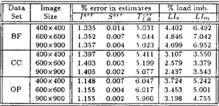
7.4 Estimated and measured percent load imbalance values, and per­ cent errors in the estimation of ray-face intersection counts (I), sampling counts (S), local rendering times (Tl r)... 52

7.5 Worst-case performance evaluation of RM-MeTiS compared to MeTiS... 52

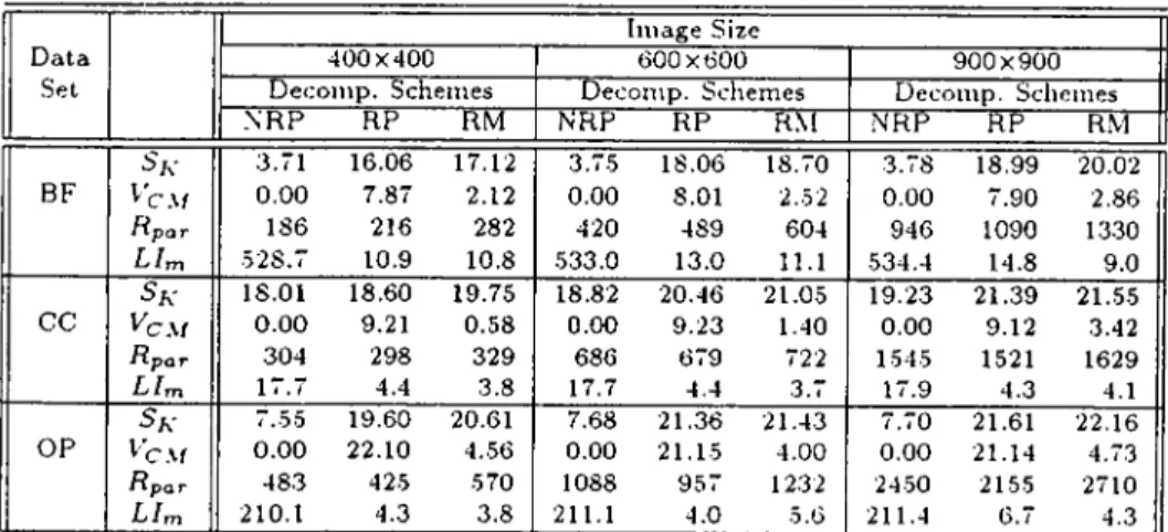
7.6 Performance comparison of various OS decomposition schemes for K=24... 54

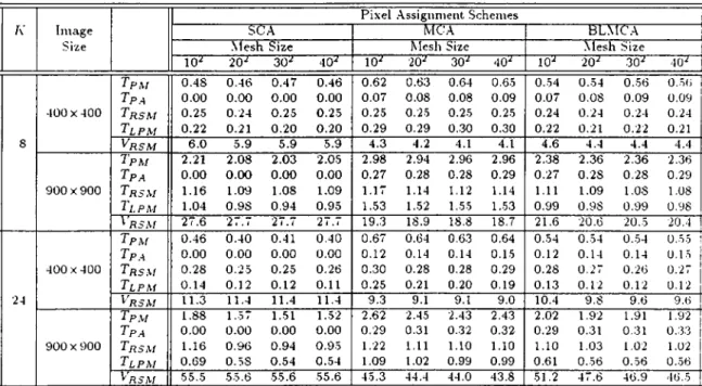
7.7 Relative performance comparison of pixel assigment ( PA ) schemes on the parallel pixel merging (PM) phase. 55

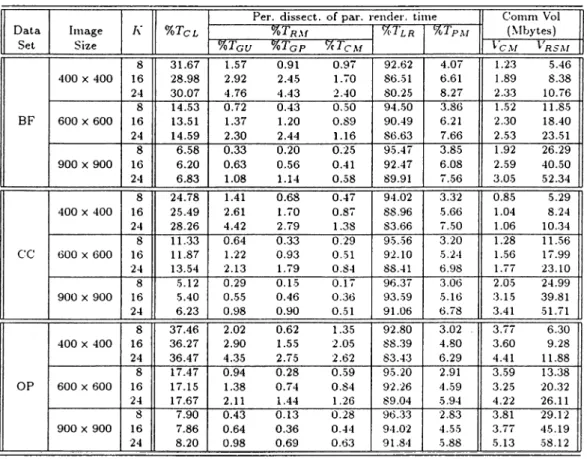
7.S View-dependent clustering overhead as a percent of view-dependent parallel rendering time Tpar, and percent dissection of Tpar- 57

C h ap ter 1

In tro d u ctio n

The increasing complexity of scientific computations and engineering simula­ tions necessitates more powerful tools for the interpretation of the acquired results. At this point, scientific visualization algorithms are utilized for the de­ tailed interpretation of the resulting datasets to reach useful conclusions. Vol­

ume rendering is a very important branch of scientific visualization and makes

it possible for scientists to visualize .3-Dimensional (3D) volumetric datasets.

Volumetric data used in volume rendering is in the form of grid superim­ posed on a volume. The vertices of this grid contain the scalar values that represent the simulation results. Type of the grid defines spatial character­ istics of the volumetric dataset, which is important in the rendering process. V'olumetric grids can be divided into two categories as: structured and un­

structured [1]. In structured grids, the distribution of grid (sample) points in

3D-space exhibit a structure. As these grids preserve a regularity in the distri­ bution of sample points, they can be represented by 3D arrays, therefore they are usually called array oriented grids. The mapping from the array elements to sample points and the connectivity relation between cells are implicit. On the other hand, in unstructured grids, the distribution of sample points do not follow a regular pattern, and there may be voids in the grid. Another term used for unstructured grids is cell oriented grids, because these grids are represented by a list of cells in which each cell contains pointers to sample points that form the cell. Due to the cell oriented nature and the irregularity of those grids,

CHAPTER 1. INTRODUCTION

the connectivity information must be provided explicitly. With the recent ad­ vances in generating higher quality adaptive meshes, unstructured grids are becoming increasingly popular in the simulation of scientific and engineering problems with complex geometries.

There are two major categories of volume rendering methods; indirect and

direct methods. Indirect methods try to track, and extract intermediate geo­

metrical representation of the data, and render those surfaces via conventional surface rendering methods. Direct methods render the data without generat­ ing an intermediate representation. However, these methods are slow due to massive computations performed, but give more accurate renderings. As the direct methods do not rely on the extraction of surfaces, they are more general and flexible.

Although volume rendering algorithms have become practical to use. there are still some problems to overcome. The most important of these problems is the speed of the rendering algorithms. Especially direct volume rendering (DVR) of unstructured grids, which is the major concern of this work, is still far from interactive response times. The slowness of the DVR process create the lack of interactivity which in turn prevents its wide use. This is one of the major reasons why there is a need for faster DVR algorithms through parallelization. In addition, it is very important for scientists to be able to change the simulation parameters so that the simulation is steered in the correct direction. Interactive visualization could help the scientists experiment with the parameters to select the useful ones.

Visualization of vast amount of volumetric dataset produced by scientific computations and engineering simulations requires large computer memory space. Hence, DVR is a good candidate for parallelization on distributed- memory multicomputers. In addition, most of the engineering simulations are done on multicomputers. Visualization of results on the same parallel machine, where simulations are done, avoids the extra overhead of transporting large amounts of data.

Existing DVR algorithms for unstructured grids can be classified into two categories; object-space and image-spcLce. In object-space methods, the volume

CHAPTER 1. INTRODUCTION

is traversed in object-space to perform a view-dependent depth sort on the cells. Then, all cells are projected onto the screen, in this visibility order, to find their contributions on the image-plane and composite them. Image-space methods are also called ray-casting methods [2, 3, 4]. In these methods, for each pi.xel of the screen, a ray is cast and followed through the volume by intersecting it with the cells to find ray-face intersections. Samples are computed along the ray and they are composited to generate the color of the pixel. For non-convex datasets, the rays may enter and exit the volume more than once. The parts of the ray that lie inside the volume, which in fact determines the contributions of the dataset to the pixel, are referred to here as ray-segments. Ray-casting approach is a desirable choice for DVR because of its capability of rendering non-convex and cyclic grids, and its power of generating images of high quality.

In this work, Koyamada’s algorithm [5], being one of the outstanding al­ gorithms of image-space methods, is selected for parallelization. Koyamada's algorithm inherently exploits the object-space coherency available in the vol­ ume through connectivity relation. Furthermore, the algorithm handles the first ray-cell intersections for ray-segment generations very efficiently by ex­ ploiting the image-space coherency. Another superiority of the algorithm is the way that it handles the resampling operations utilizing the linear sampling method. Moreover, its novel approach of determining ray-face intersections enables the use of these results in resampling phase to reduce the amount of interpolation operations.

Parallelization of ray-casting based DVR constitutes a very interesting case for domain decomposition and mapping. This application can be considered as containing two interacting domains, namely image-space and object-space. Object space is a 3D domain containing the scene (volume data) to be visual­ ized. Image space is a 2D domain containing pixels from which rays are shot into the 3D object domain to determine the color values of the respective pixels. Based on these domains, there are basically two approaches for parallel DVR;

image-space parallelism and object-space parallelism. The focus of this work is

object-space (OS) parallelism for DVR. In OS parallelism, 3D object domain is decomposed into K disjoint subvolumes and each subvolume is concurrently rendered by a distinct processor of a parallel machine with K processors. .At

CHAPTER 1. INTRODUCTION

the end of this local rendering phase, partial image structures are created at each processor. In the pixel-merging phase, these image structures are merged over the interconnection network.

Most of the previous work on parallel DVR is for structured grids. Some of these approaches and related references can be found in [6, 7, 8, 9, 10, 11. 12]. The research work on parallel DVR of unstructured grids is relatively sparse [1.3, 14, 15, 16, 17, 18]. Most of these works are for shared-memory ar­ chitectures and only Ma’s work [18] considers the parallel DVR of unstructured grids on distributed-memory architectures. The multicomputer used is an In­ tel Paragon with 128 processors. Ma’s OS-parallel algorithm uses the graph partitioning (GP) tool Chaco [19] for the OS-decomposition. Unit node and edge weighting is used in his graph model, so that the GP algorithm gener­ ates subvolumes containing equal number of cells. The ray-casting based DVR algorithm of Garrity [20] is used to render local subvolume in each processor. This static mapping is not altered when viewing parameters change. For pixel merging, image-space is evenly divided into horizontal strips, which are as­ signed to distinct processors. Pixel merging and local rendering computations are overlapped to reduce time.

The disadvantages of Ma’s OS-parallel DVR algorithm can be summarized as follows. Experimental observations indicate that having equal number of cells in each subvolume may result in extremely poor load balance due to large cell-size variations in unstructured grids. Our experimentations on benchmark volumetric datasets show that computational load imbalance can be as high as 500% on 24 processors. Similar situation holds for unit edge weighting scheme. Furthermore, the view-independent OS decomposition adopted in Ma’s algorithm does not consider the fact that the computational structure of DVR for unstructured grids substantially change with changing viewing parameters. Finally, the sequential DVR algorithm [20] employed in the local rendering computations is slow, thus hiding many overheads of the parallel implementation.

The contributions of our work can be summarized eis follows. The OS de­ composition problem for OS-parallel DVR is modeled as a GP problem with

CHAPTER 1. INTRODUCTION

correct view-dependent node and edge weighting. In the proposed model, min­ imizing the cutsize of a partition of the visualization graph corresponds to min­ imizing both the total volume of inter-processor communication during pi.xel merging computations due to ray-segment migration, and the total amount of redundant calculations during local rendering computations due to the addi­ tional ray-segments generated as a result of the partitioning. Maintaining the balance criterion corresponds to maintaining the computational load balance among processors during the local rendering computations.

As the visualization process will be carried out on the same parallel machine where simulations are done, the volumetric dataset representing the simulation results initially resides on the parallel machine in a distributed manner. How­ ever, the computational structure of parallel DVR of the first visualization instance is substantially different from that of the parallel simulation. Fur­ thermore, the computational structures of successive visualization instances with different viewing parameters may also considerably change. Thus, a new OS decomposition is necessary for each parallel visualization instance, which w'ill change the mapping of the cells of the dataset. Hence, each OS decompo­ sition should also consider the minimization of the amount of cell migration to incur because of the difference in the new and existing mappings of the cells. This problem constitutes a very typical case of a general problem known as the remapping problem. In this work, we propose a novel graph theoretical model which enables a one phase solution of the general remapping problem through GP. The proposed model generates a remapping graph by node and edge augmentations to the graph representing the computational structure of the parallel application. A MeTiS based remapping tool, which is referred to here as ReMapping-MeTiS (RM-MeTiS), is developed by modifying and enhancing the original MeTiS package for partitioning the remapping graph.

In this work, a novel OS-parallel DVR algorithm is proposed and imple­ mented. The proposed algorithm consists of four consecutive phases, namely.

clustering, remapping, local rendering and pixel merging phases. In the clus­

tering phase, GP is used for top-down clustering of the cells of the volumetric dataset to induce more tractable contracted visualization graph instances for the following view-dependent remappings. In the remapping phase, the nodes

and edges of the contracted visualization graph are weighted according to the current viewing parameter by exploiting the efficient node weight and edge weight estimation schemes proposed in this work. The contracted visualiza­ tion graph is augmented to construct the remapping graph by using the current cluster mapping. Then, the remapping graph is partitioned using R.M-MeTiS to find the new mappings for the clusters. Finally, those clusters whose new mappings differ from the current mappings migrate to their new home proces­ sors. In the local rendering phase, each processor concurrently renders its local subvolume formed by the set of local clusters by using Koyamada’s sequential algorithm. In the pixel merging pha.se. each processor produces the final im­ age of a distinct screen subregion. In this work, three screen decomposition and assignment schemes are proposed and implemented which consider the minimization of load imbalance and/or communication overhead due to ray- segment migration. Note that clustering is a view-independent preprocessing phase which is performed only once before the first visualization instance. So, the last three phases are effectively executed for the successive visualization instances.

CHAPTER 1. INTRODUCTION 6

The organization of the thesis is as follows. In Chapter 2, basic concepts of DVR, major data structures. Koyamada's DV^R algorithm and execution-time analysis of Koyamada’s algorithm are presented. Issues in OS decomposi­ tion and the GP-based OS decomposition model are discussed in Chapter 3. Chapter 4 presents the definition of the remapping problem and the proposed GP-based remapping model. The enhancements and modifications introduced to MeTiS package for developing RM-MeTiS are discussed in Chapter 5. In Chapter 6, the details of the proposed DVR algorithm are presented and dis­ cussed. Finally, Chapter 7 gives the experimental results obtained by running the proposed DVR algorithm on a Parsytec CC-24 system, which is a dis­ tributed memory multicomputer, for the visualization of benchmark volumetric datasets.

C h ap ter 2

S eq u en tial D V R A lg o rith m

In this chapter, basic concepts of DVR, major data structures, Koyainada's DVR algorithm, and execution-time analysis of Koyamada's algorithm are pre­ sented.

2.1

P relim inaries

■\ dataset is called volumetric dataset or volume data if data points of the set are defined in 3D space in a volume. The term sample point refers to a point with 3D spatial coordinates for which a numerical value is a.ssociated. Sample points in the volume data are connected in a predetermined way to form volume elements, also referred to here as cells. Sample points that form a cell are called vertices of the cell. There are various cell shapes: rectangular prism, hexahedron, tetrahedron and polyhedron being the most common ones. Our work is based on the tetrahedral cell type. A tetrahedral cell permits the direct interpolation of a point inside it by its four vertices. It also has the advantage that the data distribution is linear in any direction inside the cell. Note that other cell types mentioned can be divided into tetrahedral cells through a preprocessing step called tetrahedralization [21. 22].

In the tetrahedral cell model, each cell contains four vertices and four trian­ gular faces. The face normal is defined to be oriented outward from the parent

CHAPTER 2. SEQUENTIAL DVR ALGORITHM

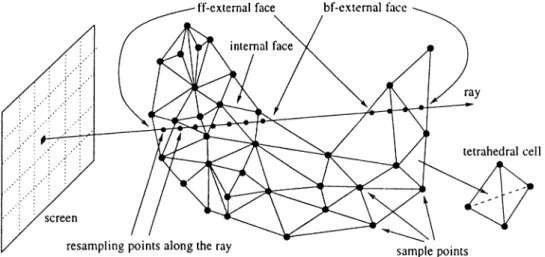
Figure 2.1; Ray-casting based direct volume rendering.

cell. If a face of a cell is shared by two cells, that face is called internal. If it is not shared by any other cell, the face is called external. A cell with at least one external face is called an external cell. Otherwise, it is called an internal

cell.

Visualization of a volumetric dataset V for the given viewing parameter t- is called a visualization instance denoted by the 2-tuple (V, e). The viewing parameter v consists of view-direction vector, view-up vector, view-reference point, view-plane window and image resolution. The vertices of the volumetric dataset V are initially in world space coordinate (WSC) system, and they are transformed into the normalized projection coordinate (NPC) system b\· using the viewing parameter t>. In NPC system. V is viewed in the positive direction, and the (.c,i/) coordinate values of vertices of V are in fact their

(.r. y) coordinate values on the image-plane. In a visualization instance (V. r).

a face of a cell of V is a front-facing (ff) face or a back-facing (bf) face if the c component of the face normal in NPC is negative or positive, respectively. In other words, a ray enters a cell through an ff-face and exits the cell through a bf-face. An external cell containing at least one ff-external face is called as a

front-external cell.

There are various types of sampling schemas in the literature. The major factors that affect the type of sampling schema used are data resolution, the variation of data values, and the variation of the transfer function. The most

common three types of schemas are: mid-point sampling, equi-distant sam­

pling, and adaptive sampling. In this work, equi-distant sampling is used. In

this schema, samples are generated at fixed intervals of length A s. Hence, for some cells more than one samples will be generated, but there will be cases such that no sample is taken in a cell. But this problem may be solved by choosing As small enough so that at least one sample wdll be taken in each cell [18]. Figure 2.1 displays the some of the concepts introduced in this section.

2.2

M ajor D a ta S tru ctu res

The first of the data structures is the data structure that stores the tetrahedral cell data. This consists of two arrays: the \ertexArray and the Cell Array.

VertexArray structure keeps the scalar values, the WSC values and the NPC

values of the vertices of the volumetric dataset. The CellArray structure keeps the following two components for each cell of the dataset:

1. A Vertices component stores the identifiers of four vertices of the cell. 2. .A NeighborCells component stores the indices of four neighbors of the cell

through its four faces and also identifies each of its internal faces by its index in the respective cell. A sentinel \alue is used for external faces. Each of the four local face indices represents a value between 0-3 which is an index to one of the four faces in the neighbor cell. This component is exploited to avoid the search for finding the entry face of the ray to the next cell during the ray-casting process.

The second major data structure is the RayBuffer. It is a 2D virtual array that holds a linked list of composited ray-segments for each pixel location of the screen. Each element of a linked list stores the following 2 components:

CHAPTER 2. SEQUENTIAL DVR ALGORITHM 9

1. A ZDeptb component which denotes the r coordinate of the exit point of the respective ray-segment. The lists are maintained in sorted increasing order according to this component.

CHAPTER 2. SEQUENTIAL DVR ALGORITHM 10

2. A Color-Opacity component which holds the composited RGB color values and the opacity value of the respective ray-segment.

2.3

K oyam ad a’s A lgorith m

Koyamada’s algorithm [5] is a ray-casting approach that makes use of the image space coherency to generate rays, and follows those rays in the object- space. Therefore, the first step of his algorithm generates the ray-segments to be traced. In his original algorithm, he sorts the ff-external faces with respect to ^ coordinates of their centroids in increasing order. This, in fact, is an approximate order, which may be wrong in some cases [5]. As the objective in this work is producing high cpiality and correct images in a fast way, this step of the original algorithm is slightly modified. Instead of sorting the external faces in the beginning, we scan convert them one by one in any order and for each pixel covered by the projection area of an ff-external face, we generate a ray-segment, traverse it through the volume for composition until it exits from a bf-external face, and finally we insert the composited ray-segment into the respective list in the RayBuffer structure.

Each ray is followed in the volume data utilizing the connectivity informa­ tion between cells. To trace a ray inside the volume, two things have to be known for each cell that is hit by the ray; the entry face and the (c,s) values at the entry point to the cell, and the exit face and the (r, s) values at the exit point from the cell. Note that the exit face and the (::,5) values at the exit point from the cell, are the entry face and the (.:,;>) values at the entry point to the next cell that the ray intersects. As for each ray-segment, the values at the point that the ray-segment first penetrates into the volume is determined during the scan conversion of ff-external faces, the problem of tracing a ra\ - segment inside the volume reduces to the problem of determining the exit point from a cell, where the entry point is given. Koyamada’s method relies on the observation that if a ray intersects a face, then the pixel that the ray is shot must be covered by the projection area of that face on the screen. So, he uses the projected area of a face to determine if the ray exits the cell from that face. His method uses the NPC values of the vertices of a face to take this decision.

CHAPTER 2. SEQUENTIAL DVR ALGORITHM 11

Consider a ray r shot from the pixel location (Xr.y,·) which intersects a tetrahedral cell ABCD through entry-point P of entry-face ABD as shown in Fig. 2.2. Let triangle ACD be the face of the cell that is subject to the ray-face intersection test. If the projection of vectors AC and AD are parallel, that is the face is perpendicular to screen, then the ray does not leave the cell through that face, so another face of the cell is tested. Otherwise, the ray r intersects the plane determined by the triangle ACD at a point Q. As the ray passes through points P and Q. (.r,j/) coordinate values (in NPC) of points P and

Q are equal to (.r^.t/r), i-e.. Xr = xp = XQ and Vr = yp = Uq ■ Then, the vector

AQ can be expressed as a linear combination of the vectors AC and AD as: AQ = aA C + fSAD.

Here, Q and (3 are weighting values, and are found by solving

(2.1) xc — xa -td — 3:a yc - Í/.4 yo - Va X a X r - Xa yr - yA ( 2.2 )

w'here {xc,yc)·, i ^D-yo) and {x a^Va) are the coordinates of points C, D and

.4 in NPC, respectively. If a and ¡3 do not satisfy the three conditions

Q>0,

¡3 > 0 and a + j3 < 1, then the point Q is not inside the triangle ACD. so

another face is tested. Otherwise, the point Q is inside the triangle ACD. so no further tests need to be done on other candidate faces. As the exit face is identified, the (.r,^i) values (-q,^^) at the exit point Q are calculated as:

= -.4 + Oi{zc - Za) — 3{zd - Í.4),

Sq = Q S c + ¡3sd -h (1 — Of — 3 )s a·

(2.3) (2.4)

Equation 2.3 is in fact writing Ecp 2.1 for the c components. Equation 2.4 is 2D inverse distance interpolation, where a . /?. and (1—a —/?) denote the ratios of areas of triangles QAD, QAC, and QCD to the area of triangle .AC'D, respectively.

As the exit-point (.Jq,S(5 ) values are computed and the entry-point {zp.sp) values are already known, the next step is to resample and composite along the ray between the entry and exit points P and Q according to the equi­ distant sampling scheme. Koyamada’s algorithm exploits the fact that the change of the scalar in any direction is linear in a tetrahedral cell to speed up

CHAPTER 2. SEQUENTIAL DVR ALGORITHM 12

Figure 2.2; Ray-face intersection and linear sampling scheme in Koyamada's algorithm.

the interpolation operations for resampling through utilizing linear sampling method. That is, the scalar value sx at each resampling point X along the line segment PQ is efficiently computed using ID inverse distance interpolation formula as sx = ’ysQ + { l —-y)sp, where 7 is the ratio of the length of the line segment PX to the length of line segment PQ. Then, the scalar value sx is mapped to a color Cx and an opacity value Ox through applying a transfer

function which converts the numerical value sx to color and opacity values to

represent the characteristics of the physical environment and simulation results. These color and opacity values are composited in front-to-back composition order as

0,+i = 0i + 0 x { \ — 0i),

C7.+1 = ( C A + C v 0 .v ( l- 0 .) ) /0 ,+ i·

(2.5) (2.6) where (C,,O.) and (C ,+i,0 ,+i) values are the composited (color,opacity) val­ ues before and after processing the resampling point A', respectively [3]. Ini­ tially, Co and Co are set to zero.

At the end of this process, the RayBuffer structure contains all the com­ posited ray-segments. The lengths of individual ray-lists in the RayBuffer structure are completely dependent on the visualization instance. If the rate of non-convexity is high for the given viewing parameters, then this means that a ray shot at a pixel has entered, and exited the volume many times. For example, the ray shown in Fig. 2.1 generates two ray-segments. For convex

CHAPTER 2. SEQUENTIAL DVR ALGORITHM 13

datasets, the length of each ray list in the Ray Buffer structure is either 0 or 1, hence the color field of the single ray-segment of each active pixel contains the final color of the respective pixel of the image. On the other hand, non-con vex datasets necessitate a final composition process over each ray-segment list of multiple length.

The nice features of Koyamada’s DVR algorithm can be summarized as follows. It makes use of image-space coherency for ray-segment generation through scan-conversion. It performs 2 ray-face intersection tests per cell on the average whereas the conventional approach always checks 3 faces [20]. It performs a ID inverse distance interpolation for each resampling, and a 2D inverse distance interpolation for each ray-cell intersection, whereas the con­ ventional approach performs expensive 3D inverse distance interpolation for each resampling. Furthermore, it uses the results of the ray-face intersection operations to reduce the amount of 2D interpolation operations.

2.4

E xecu tion T im e A nalysis

The parallelization scheme used in this work is based on graph-theoretical static decomposition and mapping of the volumetric dataset. This scheme necessitates the estimation of computational load of rendering a subvoluine for static load balancing.

The execution-time Ty of Koyamada’s algorithm for a visualization instance (V,u) can be dissected into four components, Tr, T/ and Ts- The node transformation time T/vt involves the computations for transforming WSC values of vertices to NPC values. This component can be neglected in the computational load estimation since it is extremely small compared to the total rendering time T^ (below 0.1%). The ray-segment generation time 7r involves the scan-conversion of fF-external faces to compute the intersections of ray-segments with ff-external faces and the (2,-s) values at these intersection points. The ray-face intersection time T/ involves the computation of the intersections of the ray segments with bf-faces, the scalar values, and the scalar gradients at the intersections (Eqs. 2.2- 2.4). The sampling time Ts involves

CHAPTER 2. SEQUENTIAL DVR ALGORITHM 14

the computation of the scalar values at sampling points, mapping the scalar values to colors and opacities using a transfer function and the composition of these values. Hence, the total execution time Ty can be written as;

T^ = Tn + Ti + T s ^ R^tR + Ii;ti + (2.7)

where /?y, /y and 5y denote the numbers of ray-segments generated, ray- face intersections performed and samples taken respectively. In Ecj 2.7. ¿r, ti

and ¿5 represent the unit cost of respective computations. These unit costs can not be determined through measurement because of the highly interleaved execution manner of the respective types of computations. Instead, we have estimated these unit costs statistically using the Least-Squares Approximation method. Our experimental analysis show that the average error in estimating Ty using Eq. 2.7 is below 3.5%. Efficient schemes for estimating the 7?y, 7y and 5y counts will be described in Section 6.2.1.

C h ap ter 3

Issu es in O b ject-S p a ce

D eco m p o sitio n

Koyainada’s algorithm, being an image-space method, successfully exploits the

object-space (OS) coherency through the connectivity information available in

the volume data. Therefore, the key point for a successful OS parallelization is to find an OS decomposition which maintains the OS coherency and com­ putational load balance as much as possible. In OS decomposition. .3D object domain is subdivided into disjoint subvolumes and both the computations and the data associated with all cells in each subvolume are assigned to a distinct processor for rendering. In this work, we model the OS decomposition problem as a graph partitioning problem.

3.1

Graph P artition in g (G P ) P rob lem

A weighted undirected graph 0 = €. w) is defined as a set of nodes A^, a set

of edges £ , and weighting functions w defined on nodes and edges. Every edge

Cij € £ connects a pair of distinct nodes n,· and n j . The degree d, of a node

n,· is equal to the number of edges incident to n, . The functions ic(n,) and

w(n{, Uj) denote the weights of a node U i^A f and an edge e,j e£ ■, respectively.

n = { V \,V2, ■ ■ ■ , Vk} is a K-way partition of Q if the following conditions lo

CHAPTER 3. ISSUES IN OBJECT-SPACE DECOMPOSITION 16

hold: each part Vk·, 1 < A: < A', is a nonempty subset of parts are pairwise disjoint [ VkOVi = il) for all 1 < k < C < K) , and union of K parts is equal to ^VO.e., U L i n = ^ ) . A A'-way partition is also called a multiway partition if A > 2 and a bipartition if A' = 2. A partition is said to be balanced if each part Pk satisfies the balance criterion

fbai/p(l ^ ^ I'bavffj 1 + s)? fo r k — 1 ,2 ,..., A . (3.1)

In Eq. 3.1, the size Wk of a part Vk is defined as the sum of the weights of the vertices in that part (i.e., Wk = En.6T>t ), H ai.5 = (En.e.V ii-’('6))/A

denotes the size of each part under ideal balance condition, and c represents a predetermined maximum imbalance ratio allowed.

In a partition IT of an edge is said to be cut if its pair of vertices belong to two different parts, and uncut otherwise. The set of cut edges for a partition n constitutes its edge-cut, and is denoted here as Scut- The cutsize definition for representing the cost xjlT) of a partition IT is

\(n)=

Cij^S cut

(3.2)

In Eq. 3.2, each cut edge eq contributes its cost Uj) to the cutsize. Hence.

A'-way graph partitioning problem can be defined as the task of dividing a graph into K parts such that the cutsize is minimized, while the balance criterion among part sizes is maintained.

3.2

A G P -based OS D eco m p o sitio n M odel

A visualization instance (V, v) is represented as a weighted undirected graph

Q\) = (,\/v, w’v)· The nodes in the node set A^v correspond to the cells of the dataset. Each node n, € A v corresponds to the atomic task of rendering computations associated with cell c,·. For any cell, rendering computations involve ray-face intersection tests performed on its back faces, and sampling and composition operations performed along the rays inside the cell. A front external cell involves the additional computation of ray-segment generation for its ff-external face(s), through scan-conversion. So, the computational load

CHAPTER 3. ISSUES IN OBJECT-SPACE DECOMPOSITION 17

of ail internal cell c,· and a front-external cell cj are te(n,) = E ti + Sits and

iv(nj) = Ijt[-\-Sjts + RjtR, respectively. Here, /, and 5, denote the numbers

of ray-face intersections and sampling operations associated with cell c, re­ spectively, and Rj denotes the number of ray-segments generated by the front external cell cj. Recall that i/, ts and ta are the unit costs of the respective operations (Eq. 2.7).

In the edge set £\>, e,j G £v if and only if cells c, and cj share a face / , j . In tetrahedral cell model, the given edge-set definition generates exactly one edge between each neighbor cells, since each pair of neighbor cells shares exactly one face. Furthermore, each cell can have at most four neighbor cells, hence

di < -1. Relative to the given viewing parameter v, either Ci is behind c j.

or vice versa. Here, we define the behind relation <i· such that c, <„ cj if and only if cells c,· and cj share a face fij and any ray r G R-ij intersecting face fij first hits cell cj and then hits cell c, [17]. The relation Ci <vCj also denotes that /,j is a bf-face of cell Cj, whereas it is a ff-face of cell c, . Without loss of generality let us assume that c,· is behind cj . Edge e,j represents the dependency of cell c,· to cj on the composition operations along the rays in R i j , since the composition operation is not commutative. Fortunately, this sequential nature of the composition operation can be avoided by exploiting its associativity. That is, if cells c, and cj are mapped to two distinct processors, cell c, can generate ray-segments for the rays in R.j and initiate the traversal and composition of these ray-segments without waiting the composition results of the respective rays from cell Cj. However, these partial composition results obtained by cells c, and cj for rays in Rij should be merged according to the visibility order determined by the behind relation. Hence, any cut edge e,j will incur inter processor communication because of these merge operations. The volume of communication will be proportional to the number of rays in Rij. Note that \Rij\ = Rij is in fact the number of pixels covered by the projection area of the face f i j .

Each cut edge tij will also disturb the OS coherency utilized by Koyamada’s algorithm. In Koyamada’s algorithm, for any ray r ^ R i j intersecting face f j , the exit-point ( 2, 5) values computed by cell Cj are directly used by the cell c, as the entry-point ( 2, 5) values for linear sampling and composition. So, any

CHAPTER 3. ISSUES IN OBJECT-SPACE DECOMPOSITION 18

cut edge Cij will introduce the redundant computation of entry-point (~,s) values from scratch for each ray in IZij during ray-segment generation. The amount of redundant computation will also be proportional to i?,j.

By setting the weight w{ni,nj) = Rij for each edge Cij, OS decomposition for a visualization instance, reduces to the /\-way partitioning of its associ­ ated graph according to the balance criterion (Eq. 3.1) and the cutsize definition (Eq. 3.2), where K denotes the number of processors. Each part

Vk in a partition 11 of corresponds to a subvolume V* to be rendered si­ multaneously and independently by a distinct processor Pk for 1, 2, . . . , / t . Minimizing the cutsize according to Ecp 3.2 corresponds to minimizing both the total volume of interprocessor communication and the total amount of re­ dundant computation. Maintaining the balance criterion according to Eq. 3.1 corresponds to maintaining the computational load balance among processors during local rendering calculations.

Consider a cut-edge Cij in a partition IT such that n, e Vk and c, <p Cj. Then, tij incurs the above mentioned redundant computation to processor Pk because of cell c,·. This redundant computation associated with cell c,· is same as the ray-segment generation operations performed for the front external cells in the sequential algorithm. In fact, face /,j is not shared by two cells in sub- volume V*;. and it can be considered as a ff-external face of the subvolume V*,.. Each face fij corresponding to cut edge e,j, and any cell which contains at least one such face will be referred to here as ff-boundary face and front-boundary cell, respectively. Hence, the node-weight computation scheme mentioned for front-external cells should also be used for the front-boundary cells.

3.3

R em apping P ro b lem in OS D eco m p o si­

tio n

As mentioned earlier, the main objective in parallel DVR is to visualize the volumetric datasets produced by engineering simulations and scientific com­ putations on the same parallel machine, where these computations are held.

CHAPTER 3. ISSUES IN OBJECT-SPACE DECOMPOSITION 19

So, the volumetric dataset representing the simulation results resides on the parallel machine in a distributed manner. However, this data distribution is ac­ cording to the efficient parallelization of simulation computations, which may drasticalh' differ from the decomposition criteria for efficient parallelization of DVR. Hence, a new decomposition is necessary. Furthermore, multiple vi­ sualizations of the same dataset for different viewing parameters are usually needed for a better understanding of the visualization results. However, the structure of rendering computation may substantially change with changing viewing parameters. Thus, new decompositions are also necessary between successive visualizations. However, each new decomposition and mapping may incur excessive cell migration because of the difference in the new and existing mappings of the cells. Therefore, the OS decomposition model should also consider the minimization of this data redistribution overhead. This problem constitutes a very typical case of a general problem known as the remapping

C h a p ter 4

A G P -b a sed R em ap p in g M od el

In the remapping problem, the computational structure of an application to be parallelized changes from one phase of the computation to another. The quality of the existing mapping may deteriorate both in terms of load balance and interprocessor communication. So, we should adapt the mapping in accor­ dance with these changes in the computation which necessitate the migration of computational tasks together with their associated data structures. The objective in each remapping step is to minimize the total overhead due to the task migration and the mapping of interacting tasks to different processors, while improving the load balance.

4.1

P rob lem D efinition

.A. remapping problem instance is defined by the three-tuple ( Q . M, T ) . Here,

Q = u') denotes the computational graph ¡23] representing the modified

computational structure of the application. Nodes represent atomic computa­ tions which can be executed simultaneously and independently. The weight

w{ni) of node n,· denotes the computational load of the respective task. Each

edge denotes the need for the bidirectional interaction between the respective pair of computations. The weight ty(n,, ny) of edge e,y denotes the amount of

CHAPTER 4. A GP-BASED REMAPPING MODEL 21

respective interaction. In other words, it represents the amount of communi­ cation and redundant computation to incur when n, and nj are remapped to distinct processors. M denotes the current K -way task-to-processor mapping function, where yt4 (n,·) = k means that the respective task currently resides in processor P^.. T denotes the tcisk-migration cost function, where T(ni) is the cost of migrating the respective task from its current processor Pm m to

another processor due to remapping. This cost usually refers to the communi­ cation cost for the data associated with a task.

4.2

T w o-P hase Solution M odel

A straightforward approach for solving the remapping problem is to follow a

two-phase scheme. In the first phase, K-way partitioning is performed on

graph Q as desci’ibed in Section 3.1, and a partition II is obtained. Then, n , M and T are used to construct a weighted bipartite graph for the second phase. The K parts of FI and K processors constitute the two partite nodes sets and y of the bipartite graph B = {A’,y ^£ ) such that .r*.. and y( denote part Vk and processor P(, respectively. There exist an edge between and

ye if there exists at least one task ii,· in Vk that currently resides in processor Pe (i.e.. n, e Vk and M(rii) = i). The weight of an edge t y is equal to the

sum of the migration costs of those tasks of part Vk which currently reside in processor Pe. An optimal part-to-processor assignment can be found by solving the maximum weight perfect matching problem in B. Each matched edge tke in the matching incurs the remapping of the tasks of the part Vk to processor Pe. In two phase approaches, solving the partitioning problem separately from the assignment problem usually restricts the quality of the remapping, because decisions made during the partitioning phase may prevent finding a good remapping in the second phase.

CHAPTER 4. A GP-BASED REMAPPING MODEL •y>

4.3

O n e-P hase S olution M od el

In this work, we propose a novel graph-partitioning based model for the so­ lution of the general remapping problem using a one phase approach. In the proposed model, we construct a new graph Q = {A'.S, w), referred to here as the remapping graph, through augmenting the computational graph Q. We add a node pk for each processor Pk to the node set W” of ^ to obtain the node set M oi Q. These added nodes and the original nodes of Q will be re­ ferred to here as the processor-nodes (p-nodes) and task-nodes (t-nodes) of Q. respectively. In order to obtain the edge set ^ of ^ , we augment the edge set S by connecting each p-node to those t-nodes corresponding to the tasks residing in the respective processor according the current mapping function yVf. These added edges and the original edges will be referred to here as processor-to-task edges (pt-edges) and task-to-task edges (tt-edges), respectively. That is,

jif = J^^l) jCp and £ = ¿^^[J ¿p, where (4.1)

Aft = M and Afp = { pi ,p2<---- Pa'}, (4.2)

£tt = £ and £pt = {{ni,pk) : n,· G A’i.pjt G A'p and M(ni) = k}. (4.3)

In node weighting, weights of t-nodes remain the same, whereas p-nodes are assigned zero weights. In edge weighting, weights of tt-edges remain the same, whereas each pt-edge will be assigned the task-migration cost of the respective task. That is,

w(ni) = iv(ni) y n i^ A ft and w{pk) = 0 '^Pk^Afp, (4.4)

ih{n,.pk) = T{ni) 'icik^Aipt and w (ni.nj) = w{iii,nj) Ve,j G ;V'’„.(4.5)

A A'-way partition fl = {V i,V2·, · · ·, Vk} of graph Q is defined to be feasible

if it satisfies the mapping constraint

V k = L - 2 . . . . , K . (4.6) That is, each part Vk of IT contains exactly one p-node. Then, a feasible partition n of ^ induces the remapping M in which tasks corresponding to the t-nodes in each part are all assigned to the same processor corresponding to the unique p-node in that part. That is, yW(n,) = k if both the t-node n, and the p-node pk are in the same part of II.

CHAPTER 4. A GP-BASED REMAPPING MODEL 23

One phase solution to the remapping problem reduces to the /\-way parti­ tioning of graph ^ according to the mapping constraint (Eci. 4.6), balance cri­ terion (Eci· 3.1), and the cutsize definition (Eq. 3.2). Maintaining the balance criterion corresponds to maintaining the computational load balance among processors, since p-nodes are assigned zero weights. Minimizing the cutsize corresponds to minimizing the total overhead due to task migration and inter­ actions between tasks mapped to different processors. Note that there might be two types of edges in the edge-cut. A tt-edge eq in the edge-cut incurs communication between processors Pj\;^(n,) ^M(nj) because of the inter­

actions between atomic tasks corresponding to the t-nodes n, and iij. Such tt-edges in the edge-cut may also incur redundant computations. A pt-edge e,t in the edge-cut incurs interprocessor communication due to migration of the task corresponding to the t-node n,· from processor P^ to processor PjCn„^y Note that the task-migration cost function T should be wisely selected to in­ corporate the appropriate scaling between weights of tt-edges and pt-edges. In the absence of redundant computation, the scaling can be inherently solved by weighting both types of edges in terms of their relative communication volume requirements.

The proposed graph-partitioning based remapping model is e.xploited for OS decomposition in our parallel DVR. In the OS decomposition, the remapping instance is identified by three-tuple (^y..V f,T ). Here the graph t/y represents the computational structure of the visualization instance (V, c) as mentioned in Section 3.2. M is the current cell-to-processor mapping inherited either from the parallel simulation or the previous parallel visualization. The cell- migration cost T can be constructed through a scaling which considers only the communication volume overhead. So, T(ni) can be set equal to the ratio of the size of the data associated with cell c,· to the size of an individual ray- segment information.

C h a p ter 5

M eT iS -b a sed R em a p p in g

H eu ristic

5.1

G raph P a rtitio n in g H eu ristics

Kernighan-Lin (KL) based heuristics are widely used for graph/hypergraph partitioning because of their short run-times and good quality results. KL algorithm is an iterative improvement heuristic originally proposed for bipar­ titioning [2-1]. KL algorithm, starting from an initial bipartition, performs a number of passes until it finds a locally minimum partition. Each pass consists of a sequence of vertex swaps. Fiduccia-Mattheyses (FM) [25] introduced a faster implementation of KL algorithm by proposing vertex move concept in­ stead of vertex swap. This modification as well as proper data structures, e.g.. bucket lists, reduced the time complexity of a single pass of KL algorithm to linear in the size of the graph.

The performance of FM algorithms deteriorates for large and too sparse graphs. Furthermore, the solution quality of FM is not stable (predictable), i.e., average FM solution is significantly worse than the best FM solution, which

CHAPTER 5. METIS-BASED REMAPPING HEURISTIC ■lo

is a common weakness of move-based iterative improvement approaches. Ran­ dom multi-start approach is used in VLSI layout design to alleviate this prob­ lem by running FM algorithm many times starting from random initial parti­ tions to return the best solution found [26]. However, this approach is not viable in parallel computing since decomposition is a preprocessing overhead intro­ duced to increase the efficiency of the underlying parallel algorithm/program. Most users will rely on one run of the decomposition heuristic, so that the quality of the decomposition tool depends equally on the worst and average decompositions than on just the best decomposition.

Recently, multilevel grAph. partitioning methods have been proposed leading to successful graph partitioning tools Chaco [19] and MeTiS [27]. These mul­ tilevel heuristics consists of .3 phases, namely coarsening, initial partitioning, and uncoarsening. In the first phase, multilevel clustering is successively ap­ plied starting from the original graph by adopting various matching heuristics until number of vertices in the coarsened graph reduces below a predetermined threshold value. In the second phase, coarsest graph is partitioned using vari­ ous heuristics including FM. In the third phase, partition found in the second phase is successively projected back towards the original graph by refining the projected partitions on intermediate level uncoarser graphs using various heuristics including FM.

5.2

M od ifyin g M eT iS Package for R em apping

In this work, we exploit the state-of-the-art MeTiS graph partitioning tool (KMeTiS option) to partition the remapping graph Q for solving the A'-way remapping problem. However, MeTiS can not handle the mapping constraint (Eq. 4.6) directly. In this section, we present our modifications and enhance­ ments to each phase of the MeTiS package to make it support the mapping constraint. This version of MeTiS will be called as ReMapping-MeTiS (RM- MeTiS).

CHAPTER 5. METIS-BASED REMAPPING HEURISTIC 26

5.2.1

C oarsen in g P h ase

In this phase of MeTiS, the given graph 0 = Oo = {J^o,SQ, ibo) is coarsened into a sequence of smaller graphs , Q2 = (Л 2,¿21 ^ ····

Qm = Satisfying |7^o| > |A''il> |. \ 2| > ... > lACrJ, until reduces below a threshold value. This coarsening is achieved by coalescing disjoint subsets of vertices of graph Qe, into supernodes of next level graph Qt+\ through various randomized matching schemes. The weight of each supernode of is set equal to the sum of its constituent nodes in 0(. The edge set of each supernode is set equal to the weighted union of the edge sets of its constituent nodes. In randomized matching, nodes of Q( are visited in a random order. If a node n, has not been matched yet, one of its unmatched

adjacent nodes is selected according to a criterion. If such a node nj exists,

the matched pair n, and nj is merged into a supernode of . If there is

no unmatched adjacent node of n,·, then node nj remains unmatched. Among various matching criteria available in MeTiS, the heavy edge matching scheme (HEM) is selected for RM-MeTiS. In HEM, a node n,· is matched with node

nj such that the weight of the edge between these two nodes, is maximum over

all valid edges incident to node n,·.

.At each level i of the coarsening phase of MeTiS, the coarse graph Qf, effec­ tively induces a |AV|-way partition of the original graph Qo- The idea behind R.\l-MeTiS, is to maintain the mapping constraint (Eq. 4.6) in a relatively relaxed manner such that the node cluster corresponding to each supernode of Of. contains at most one p-node of the original graph Qq. In RM-MeTiS.

we maintain a flag for each node to indicate whether it is a t-node or p-node. Matching two t-nodes in Q(, produces a t-supernode in , whereas matching a t-node with a p-node produces a p-supernode. In randomized HEM match­ ing. two unmatched supernodes are considered for matching only if at least one of them is a t-supernode. That is, at any coarsening level (!, the constituent nodes of a t-supernode in Qe are all t-nodes whereas the constituent nodes of a p-supernode in Qe are all t-nodes except one p-node. Note that there exist exactly К p-supernodes in at each level i during the coarsening phase.

CHAPTER 5. METIS-BASED REMAPPING HEURISTIC 21

5.2.2

In itia l P a rtitio n in g P hase

The objective of this phase is to find a good K -way partition of the coarsest graph Qrn which minimizes the cutsize (Eq. 3.2) while maintaining the balance criterion (Eq. 3.1). KMeTiS [28] constructs a A'-way partition of Qm by re­ cursive bisection using the multilevel bisection algorithm PMeTiS [29]. In this scheme, first a 2-way partition of Om is obtained, and then this bipartition is further partitioned in a recursive manner. After lg2 K phases graph Q,n partitioned into K parts.

In RM-MeTiS, the objective of the initial partitioning phase is to find a good A'-way partition of graph Qm which satisfies the mapping constraint (Eq. -1.6) in addition to the pure graph-partitioning criteria (Eqs. 3.2 and 3.1). In RM-MeTiS, we adopt a direct A'-way partitioning scheme instead of recur­ sive bisection scheme of original MeTiS because of the following two reasons. First, it is harder to maintain the mapping constraint during the recursive bi­ section steps. Second, the intrinsic features of coarsest graph can be efficiently exploited in direct A'-way partitioning as described below.

The most successful initial partitioning algorithm in PMeTiS is reported to be the greedy graph growing algorithm (GGGP). GGGP algorithm starts from an initial bipartition where a randomly selected node and all the remaining nodes constitute the bipartitioning. The former and later parts are referred here as growing and shrinking parts. Then, boundary nodes of the shrinking part are moved to the growing part according to their EM gains until the balance criteria becomes satisfied. The EM gain of a node move is defined as the decrease in the cutsize if the move is realized. A positive gain means a decrease, whereas a negative gain means an increase in the cutsize. A node in a part is said to be a boundary node if it is incident to at least one cut-edge in the partition.

The performance of GGGP algorithm is sensitive to the choice of the initial node. The extension of GGGP algorithm to A'-way partitioning requires the selection of A' — 1 such nodes for the initial growing parts, which may degrade the performance in the general partitioning Ccise. Fortunately, the property that contains exactly K p-supernodes and ]A''m|-A' t-supernodes can