PARALLEL-MLFMA SOLUTION OF CFIE DISCRETIZED
WITH TENS OF MILLIONS OF UNKNOWNS
¨
O. Erg ¨ul
1,2, L. G ¨urel
1,21Department of Electrical and Electronics Engineering 2Computational Electromagnetics Research Center (BiLCEM)
Bilkent University, TR-06800, Bilkent, Ankara, Turkey E-mail: [email protected], [email protected]
fax: +90-312-2905755
Keywords: Electromagnetic scattering, combined-field integral equation, multilevel fast multipole algorithm, large-scale problems, parallelization.
Abstract
We consider the solution of large scattering problems in electromagnetics involving three-dimensional arbitrary geometries with closed surfaces. The problems are formulated accurately with the combined-field integral equation and the resulting dense matrix equations are solved iteratively by employing the multilevel fast multipole algorithm (MLFMA). With an efficient parallelization of MLFMA on relatively inexpensive computing platforms using distributed-memory architectures, we easily solve large-scale problems that are discretized with tens of millions of unknowns. Accuracy of the solutions is demonstrated on scattering problems involving spheres of various sizes, including a sphere of radius 110λ discretized with 41,883,638 unknowns, which is the largest integral-equation problem ever solved, to the best of our knowledge. In addition to canonical problems, we also present the solution of real-life problems involving complicated targets with large dimensions.
1 Introduction
Surface integral equations are commonly used to formulate scattering problems involving three-dimensional conductors with arbitrary shapes [24]. When the scatterer involves closed surfaces, the combined-field integral equation (CFIE) is usually preferred to formulate the problem. This is because CFIE is free of the internal resonances [22] and it provides better-conditioned matrix equations than the electric-field integral equation (EFIE) and the magnetic-field integral equation [17],[31]. Simultaneous discretizations of the scatterer and CFIE lead to dense matrix equations, which can be solved iteratively using efficient acceleration methods, such as the multilevel fast multipole algorithm (MLFMA) [27]. However, accurate solutions of many real-life problems
require discretizations with millions of elements leading to matrix equations with millions of unknowns. To solve these large problems, it is helpful to increase computational resources by parallelizing MLFMA. Recently, there have been many efforts to develop parallel implementations of MLFMA running on clusters of computers connected via fast networks [30]. Thanks to these efforts, it has become possible to solve 20–30 million unknowns on relatively inexpensive computing platforms [18],[19],[28]–[30].
In this paper, we present our efforts to develop a sophisticated simulation environment based on MLFMA for the solution of large-scale scattering problems formulated by CFIE. Efficient and accurate solutions require a multidisciplinary study involving diverse components, such as discretization, iterative algorithms, preconditioners, and parallelization. For numerical solutions, we model the surfaces by using small planar triangles. Then, we employ linear basis functions, such as Rao-Wilton-Glisson (RWG) [25] functions, to expand the unknown surface current density. Formulation of closed surfaces with CFIE usually leads to well-conditioned matrix equations that are easy to solve iteratively. We further improve the iterative convergence by employing efficient preconditioners. For the solution of large-scale problems involving complicated structures, we implement a parallel version of MLFMA that is suitable for use on clusters of personal computers. By achieving an efficient parallelization of MLFMA, we are able to solve problems with tens of millions of unknowns. As an example, we present the results of a scattering problem involving a sphere of radius 110λ discretized with 41,883,638 unknowns, the largest integral-equation problem solved to date. We also demonstrate the effectiveness of our simulation environment by presenting examples on scattering problems involving a complicated target with a size larger than 300λ.
2 Combined-Field Integral Equation (CFIE)
For perfectly conducting objects, EFIE can be written directly by testing the boundary condition for the tangential electricfield on the surface as −ik ˆt · Z S dr0J(r0) ·³I −∇∇0 k2 ´ g(r, r0) = 1 ηˆt · E inc(r), (1) where the scattered electric field is expressed in terms of the induced (unknown) surface current J(r), ˆt is any tangential
unit vector on the surface at the observation point r, Einc(r) is the incident electric field, η is the impedance of free space,
k is the wavenumber, and gl(r, r0) =e
ikR 4πR
³
R = |r − r0|´ (2) denotes the free-space Green’s function in phasor notation with the e−iwt convention. For closed surfaces, MFIE can be formulated similarly (by using the boundary condition for the tangential magnetic field) as
J(r) − ˆn ×
Z S
dr0J(r0) × ∇0g(r, r0) = ˆn × Hinc(r), (3) where the observation point r approaches the surface from the outside, ˆn is the outwardly directed normal, and Hinc(r) is the incident magnetic field. In the case of EFIE, the tangential component of the electric field is directly sampled (tested) on the surface by using the tangential unit vector ˆt. On the
other hand, MFIE is constructed by using a cross product with the outward normal vector ˆn to obtain the tangential
magnetic field on the surface of the scatterer. The alternative choices, i.e., testing the fields by using the normal and the tangential unit vectors for EFIE and MFIE, respectively, usually produce extremely ill-conditioned matrix equations, when the discretization is performed by using a Galerkin scheme.
For the solution of problems involving closed surfaces, both EFIE and MFIE suffer from the internal-resonance problem and they do not provide unique solutions at resonance frequencies related to the geometrical properties of the closed conductors [22]. To alleviate this problem, EFIE and MFIE are combined to obtain CFIE as
CFIE = α(r)EFIE +£1 − α(r)¤MFIE, (4) where α(r) is chosen in the range from 0.0 to 1.0 depending on the observation (testing) point on the surface. For composite structures involving both open and closed surfaces, EFIE (α(r) = 1) is used for the open parts, while MFIE is activated in addition to EFIE (0 < α(r) < 1) for the closed parts. The scatterers considered in this paper involve only closed surfaces. Consequently, we use α(r) = 0.2 for all testing points, which is usually an optimal choice for the convergence rate of the iterative solutions [7]. Compared to EFIE and MFIE, CFIE is not only free of the internal resonance problem, but also provides well-conditioned matrix equations that are crucial for iterative solvers, such as MLFMA [17]. In addition, iterative convergence of CFIE solutions can be further accelerated by using simple and cost-efficient preconditioners.
3 Discretization of CFIE
For the numerical solution of CFIE, the unknown current density on the surface of the scatterer is expanded in a series of basis functions bn(r), i.e.,
J(r) =
N X n=1
anbn(r), (5) where an is the unknown coefficient of nth basis function. Then, the boundary conditions are enforced by a projection onto the testing functions tm(r) and N × N matrix equations are obtained as
N X n=1
ZmnC an = vCm, m = 1, ..., N. (6) In (6), matrix elements are derived as
ZC mn= αmZmnE + (1 − αm)ZmnM , (7) where ZE mn= −ik Z Sm drtm(r) · Z Sn dr0b n(r0)g(r, r0) + i k Z Sm drtm(r) · Z Sn dr0b n(r0) · h ∇∇0g(r, r0)i (8) and ZM mn= Z Sm drtm(r) · bn(r) − Z Sm drtm(r) · ˆn × Z Sn dr0b n(r0) × ∇0g(r, r0) (9) are the contributions of EFIE and MFIE, respectively. Sim-ilarly, elements of the right-hand-side vector can be written as vC m= αmvEm+ (1 − αm)vmM = Z Sm drtm(r) · h αm η E inc(r) + (1 − α m)ˆn × Hinc(r) i . (10) In (8)–(10), Sm and Sn represent the supports of the mth testing and nth basis functions, respectively.
In this paper, surfaces are discretized by using small triangles, on which RWG functions are defined. We use the same set of RWG functions as the basis and testing functions according to a Galerkin scheme. The matrix elements in (7)–(9) can be interpreted as the interactions between the basis and testing functions. In the MLFMA implementations, there are O(N ) near-field interactions that are calculated directly by evaluating the integrals in (8) and (9). In general, we perform the following steps for the efficient and accurate calculation of these interactions:
1) The loops are constructed over the triangles instead of the functions. In such a construction, the integrals over the basis and testing functions must be divided into many
basic (double) integrals that are independent from the alignment of the functions [6].
2) The inner integrals in the forms of
I1= Z St dr0 x10 y0 g(r, r0) (11) I2= Z St dr0 x10 y0 ∇0g(r, r0), (12) are evaluated accurately by using singularity extraction techniques [14],[20],[23], Gaussian quadratures [5], and adaptive integration methods [6]. Then, the inner inte-grals are used in forming the integrands of the outer integrals.
3) The outer integrals are calculated by using Gaussian quadratures and adaptive integration methods. For MFIE part of the matrix elements, a singularity extraction technique is applied for some of the outer integrals to improve the accuracy and efficiency of the calcula-tions [16].
4 Multilevel Fast Multipole Algorithm
The dense matrix equation in (6) can be solved iteratively, where the matrix-vector multiplications (MVMs) are acceler-ated by employing MLFMA. In general, MLFMA splits the MVMs as [27]
ZC· x = ZCN F · x + Z C
F F · x, (13)
where the near-field interactions denoted by ZCN F are calcu-lated directly and stored in memory, while the far-field in-teractions (ZCF F) are computed approximately in a group-by-group manner. For a single-level fast multipole algorithm [4], far-field interactions can be written as
ZmnC = ik (4π)2 Z d2ˆkFCm(ˆk) αT(k, RCC0) · GC0n(ˆk) (14) where ˆk is the angular direction on the unit sphere, k = kˆk,
and αT(k, RCC0) = T X t=0 it(2t + 1)h(1) t (kRCC0)Pt(ˆk · ˆRCC0) (15) is the translation function written in terms of the spherical Hankel function of the first kind h(1)t and the Legendre polynomial Pt. The translation function in (15) evaluates the interaction between the basis and testing groups that are located at C0 and C, respectively, and separated by
RCC0 = |RCC0| ˆRCC0 = rC− rC0. (16) In (14), GC0n(ˆk) = ¡ I − ˆkˆk¢· Z Sn dr0exp [−ik · (r0− r C0)]bn(r0) (17)
is the radiation pattern of the nth basis function with respect to a nearby reference point C0 [3]. Similarly,
FCm(ˆk) = h
αmFECm(ˆk) + (1 − αm)FMCm(ˆk) i
(18) represents the receiving pattern of the mth testing function with respect to a reference point C, where
FE Cm(ˆk) = ¡ I − ˆkˆk¢· Z Sm dr exp [ik · (r − rC)]tm(r) (19) and FMCm(ˆk) = −ˆk × Z Sm dr exp [ik · (r − rC)]tm(r) × ˆn(r). (20) Using the RWG functions, the integrals in (18)–(20) can be evaluated analytically.
In MLFMA, the interactions in (14) are calculated in a multilevel scheme using a tree structure constructed by including the scatterer in a cubic box and recursively dividing the computational domain into subboxes. The tree structure of MLFMA includes L = O(log N ) levels. At level l from 1 to L, the number of nonempty boxes (clusters) is Nl, where
N1= O(N ) and NL= O(1). Each MVM involves four main stages that are performed as follows.
• Near-field interactions: In MLFMA, there are O(N ) near-field interactions that are used to perform the multiplica-tion
y = ZCN F · x. (21) These interactions are calculated and stored in the mem-ory before the iterative solution.
• Aggregation: Radiated fields at the centers of the clusters are calculated from the bottom of the tree structure to the highest level. The fields are sampled uniformly in the φ direction, while we use the Gauss-Legendre quadrature in the θ direction [4]. To determine the number of samples required for a desired level of accuracy, we use the excess bandwidth formula considering the worst-case scenario according to a one-box-buffer scheme [21]. Oscillatory nature of the Helmholtz solutions requires that the sam-pling rate depends on cluster size as measured by the wavelength (λ = 2π/k). During the aggregation stage, we employ local Lagrange interpolation method to match the different sampling rates of the consecutive levels [10]. The radiation patterns of the basis functions are calculated and stored in the memory before the iterative solutions. • Translation: Radiated fields are translated into incoming
fields. For a basis cluster at any level, there are O(1) testing clusters to translate the radiated field. In addition, using cubic (identical) clusters, there is a maximum of 73− 33 = 316 different translations in each level,
independent of the number of clusters [29]. Similar to the radiation and receiving patterns, translation operators defined in (15) are also calculated and stored in memory
before the iterations. We employ interpolation methods to calculate these operators in O(N ) time [9],[26]. • Disaggregation: The incoming fields at the centers of the
clusters are calculated from the top of the tree structure to the lowest level. The sampling scheme for the incoming fields is the same as the sampling scheme for the radiated fields calculated during the aggregation stage. Different from the aggregation stage, however, sampling rates of the consecutive levels are matched by using transpose interpolation (anterpolation) [2]. At the lowest level, the incoming fields are multiplied by the receiving patterns of the testing functions. Similar to the radiation patterns of the basis functions, the receiving patterns are also calculated and stored in the memory before the itera-tive solution. Finally, the angular integration in (14) is performed to complete the MVM.
Since the memory requirement and the processing time required for each level of MLFMA are proportional to N , the overall complexity of the MVMs is O(N log N ) [27]. The complexity of the setup, which involves the construction of the multilevel tree and calculation of the data required during the MVMs (near-field interactions, radiation and receiving patterns of the basis and testing functions, and the translation operators) is O(N ).
5 Iterative Solvers and Preconditioners
For the iterative solutions accelerated by MLFMA, we employ Krylov subspace methods, such as conjugate gradient (CG), conjugate gradient squared (CGS), biconjugate gradient (BiCG), stabilized BiCG (BiCGStab), quasi-minimal residual (QMR), transpose-free QMR (TFQMR), generalized minimal residual (GMRES), and least-square QR (LSQR) algorithms [1]. For a given problem, performance of each algorithm may vary significantly, depending on the shape of the geometry, discretization, and the type of the formulation. Since reducing the number of iterations is extremely important to obtain efficient solutions, we investigate and compare the iterative solutions provided by various algorithms. For the solution of scattering problems formulated with CFIE, we prefer GMRES and BiCGStab, which usually perform better than other algorithms [13]. In addition, we further accelerate the iterative convergence by employing preconditioners and modifying the original matrix equation as
M−1Z · a = M−1v (22) by multiplying both sides with M−1. In (22), M is a preconditioner matrix constructed by using some of the near-field interactions. Due to its favorable computing cost, we usually employ the block-diagonal preconditioner (BDP) [27] obtained by selecting only the self interactions of the lowest-level clusters. For the solution of the matrix equations obtained by CFIE, BDP reduces the number of iterations significantly.
6 Parallelization of MLFMA
Many real-life scattering problems formulated by integral equations require the solution of matrix equations with millions of unknowns. For the solution of these large-scale problems, it is helpful to increase computational resources by assembling parallel computing platforms and at the same time by parallelizing the solvers. Of the various parallelization schemes for MLFMA, the most popular use distributed-memory architectures by constructing clusters of computers with local memories connected via fast networks [30]. However, parallelization of MLFMA is not trivial. Simple parallelization strategies usually fail to provide efficient solutions because of the communications between the processors and the unavoidable duplication of some of the computations over multiple processors.
A simple parallelization of MLFMA involves the distribution of the clusters among the processors [8]. In this scheme, each cluster at any level is assigned to a single processor. For an efficient parallelization of MLFMA, it is essential to distribute the tree structure among the processors with minimal duplication and communication between the processors. In this manner, the simple strategy works efficiently for the lower levels, which include many clusters with low sampling rates for the fields. Problems arise in the higher levels involving small numbers of clusters with large sampling rates.
1) It is difficult to distribute small numbers of clusters in the higher levels with a good load balance. To avoid communications during the aggregation and disaggre-gation stages, the clusters in the higher levels should be duplicated in multiple processors. Even using load-balancing algorithms, these duplications may deteriorate the efficiency of the parallelization dramatically, since these clusters have large numbers of samples for the fields.
2) Distributing the clusters among the processors, the translations involve dense one-to-one communications between the processors. The amount of the transferred data can be very large in the higher levels, which may also reduce the parallelization efficiency significantly. Identifying the problems of the simple strategy as described above, a hybrid partitioning approach employs different parti-tioning strategies for the lower and higher levels to improve the parallelization efficiency [30]. In this technique, processor assignments are made on the basis of the fields of the clusters in the higher levels. Then, each cluster in these levels is shared by all processors and each processor is assigned to the same portion of the fields of all clusters. Since the fields in the higher levels have large sampling rates, the samples can be distributed efficiently among the processors. In addition, dense one-to-one communications between the processors during the translations are eliminated. On the other hand, distributing fields among the processors introduces new communications during the aggregation and disaggregation stages. These
com-170 172.5 175 177.5 180 −20 −10 0 10 20 30 40 50 60 Total RCS (dB) Analytical Computational
80λ
170 172.5 175 177.5 180 −20 −10 0 10 20 30 40 50 60 Total RCS (dB) Analytical Computational96λ
170 172.5 175 177.5 180 −20 −10 0 10 20 30 40 50 60 Total RCS (dB) Bistatic Angle Analytical Computational110λ
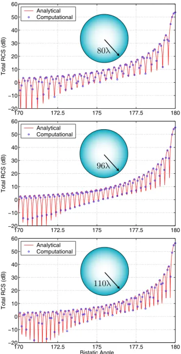
Fig. 1: Bistatic RCS (in dB) of spheres of radii 80λ, 96λ, and 110λ from 160◦ to 180◦, where 180◦ corresponds to the forward-scattering direction.
munications are performed to transfer relatively small amounts of data required for the interpolations and produced by the anterpolations, and their extra cost is usually unimportant when the number of processors is small (1 to 16). For the solutions using large numbers of processors, however, the hybrid parallelization may become inefficient due to increasing amount of the transferred data during the aggregation and disaggregation stages. For these solutions, a hierarchical parti-tioning approach based on appropriate partiparti-tioning of both the samples of the fields and the clusters for all levels can provide high efficiency [12]. Diameter 160λ 192λ 220λ Unknowns 23,405,664 33,791,232 41,883,648 Setup (minutes) 94 183 274 BiCGStab Iterations 17 21 19 MVM (seconds) 270 372 441 Solution (minutes) 155 264 290 Total Memory (GB) 113 184 229 Relative Error 4.4% 4.5% 4.7%
Table I: Solutions of large sphere problems with MLFMA parallelized into 16 processes.
7 Results
By constructing a sophisticated simulation environment based on parallel MLFMA, we are able to solve scattering problems discretized with tens of millions of unknowns. As an example, we present the solution of large scattering problems involving spheres of radii 80λ, 96λ, and 110λ, which are discretized with 23,405,664, 33,791,232, and 41,883,648 unknowns, re-spectively, using λ/10 triangulation. For all three problems, 9-level MLFMA is employed and parallelized into 16 processes running on a cluster of quad-core Intel Xeon 5355 processors connected via an Infiniband network. Using a top-down strat-egy, the cluster size in the lowest level is 0.16λ–0.21λ. We use the hybrid parallelization approach to distribute the tree structures among the processors. Both the near-field and the far-field interactions are calculated with 1% error. In Table I, we present the processing time and the total memory usage for the solution of the sphere problems. Using BDP, the number of BiCGStab iterations to reduce the residual error below 10−3is 17–21. For the largest problem with 41,883,648 unknowns, the setup and the iterative solution parts take about 274 and 290 minutes, respectively, and the total memory usage is 229 GB using the single-precision representation to store the data. To present the accuracy of the solutions, Fig. 1 depicts the normalized bistatic radar cross section (RCS/λ2) values in
decibels (dB) for the spheres. Analytical values obtained by Mie-series solutions are also plotted as a reference from 160◦ to 180◦, where 180◦ corresponds to the forward-scattering direction. Fig. 1 shows that the computational values sampled at 0.1◦ are in agreement with the analytical curves. For more quantitative information, we define a relative error as
eR= ||A − C||2
||A||2
, (23) where A and C are the analytical and computational values of the far-zone electric field, respectively, ||.||2 is the l2-norm
defined as ||x||2= v u u tXS s=1 ¯ ¯x[s]¯¯2 , (24) and S is the number of samples. As also listed in Table I, the relative error is smaller than 5% in the 160◦–180◦ range for all three solutions. This error is mostly due to
y
x
Fig. 2: A stealth airborne target Flamme.
the discretization of CFIE with the RWG functions and the accuracy can be improved by employing higher-order linear-linear basis functions [11].
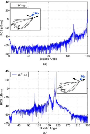
Next, we present solutions of a real-life problem involving the Flamme, which is a stealth airborne target, as detailed in [15] and also depicted in Fig. 2. The scattering problem is solved at 16 GHz and the maximum dimension of the Flamme is 6 meters, corresponding to 320λ. Using λ/10 triangulation, the problem is discretized with 24,782,400 unknowns. Solutions are performed by a 10-level MLFMA parallelized into 16 processes. The nose of the target is in the x direction. Fig. 3(a) presents the co-polar RCS values in dBm2 on the x-y plane as a function of the bistatic angle φ,
when the target is illuminated by a plane wave propagating in the −x direction with the electric field polarized in the y direction (φ polarization). In the plots, 0◦ and 180◦ correspond to the back-scattering and forward-scattering directions, respectively. In Fig. 3(b), the bistatic RCS values are plotted from 0◦ to 360◦ when the target is illuminated by a plane wave propagating in the x-y plane at a 30◦ angle from the x axis (from φ = 30◦). In this plot, 30◦ and 210◦ correspond to the back-scattering and forward-scattering directions, respectively. After the setup, which takes about 104 minutes, the problem is solved twice (for two excitations) in about 470 minutes. Using BiCGStab and BDP, the numbers of iterations to reduce the residual error below 10−3 are 36 and 35 for the illuminations from φ = 0◦ and φ = 30◦, respectively.
8 Conclusion
In this paper, we consider fast and accurate solutions of large-scale scattering problems formulated by CFIE. Using a parallel implementation of MLFMA, we are able to solve problems discretized with tens of millions of unknowns. We demonstrate the accuracy and efficiency of our implementations by considering both canonical and real-life problems, including a sphere of radius 110λ and the stealth Flamme geometry with a size larger than 300λ.
Acknowledgements
This work was supported by the Scientific and Technical Research Council of Turkey (TUBITAK) under Research
0 45 90 135 180 −80 −60 −40 −20 0 20 40 RCS (dBms) Bistatic Angle 0o−φφ (a) 0 45 90 135 180 225 270 315 360 −80 −60 −40 −20 0 20 40 RCS (dBms) Bistatic Angle 30o−φφ (b)
Fig. 3: Bistatic RCS (in dBm2) of the stealth airborne target
Flamme at 16 GHz. Maximum dimension of the Flamme is 6 meters corresponding to 320λ. The target is illuminated by a plane wave propagating (a) in the −x direction and (b) in the x-y plane at a 30◦angle from the x axis, as also depicted in the insets.
Grant 105E172, by the Turkish Academy of Sciences in the framework of the Young Scientist Award Program (LG/TUBA-GEBIP/2002-1-12), and by contracts from ASELSAN and SSM. Computer time was provided in part by a generous allocation from Intel Corporation.
References
[1] S. Balay, K. Buschelman, V. Eijkhout, W. D. Gropp, D. Kaushik, M. G. Knepley, L. C. McInnes, B. F. Smith, and H. Zhang, PETSc Users Manual, Argonne National Laboratory, 2004.
[2] A. Brandt, “Multilevel computations of integral trans-forms and particle interactions with oscillatory kernels,”
Comp. Phys. Comm., vol. 65, pp. 24–38, Apr. 1991.
[3] W. C. Chew, J.-M. Jin, E. Michielssen, and J. Song, Fast
Electromag-netics. Boston, MA: Artech House, 2001.
[4] R. Coifman, V. Rokhlin, and S. Wandzura, “The fast multipole method for the wave equation: a pedestrian prescription,” IEEE Ant. Propag. Mag., vol. 35, no. 3, pp. 7–12, Jun. 1993.
[5] D. A. Dunavant, “High degree efficient symmetrical Gaussian quadrature rules for the triangle,” Int. J.
Nu-mer. Meth. Eng., vol. 21, pp. 1129–1148, 1985.
[6] ¨O. Erg¨ul, “Fast multipole method for the solution of elec-tromagnetic scattering problems,” M.Sc. thesis, Bilkent University, Ankara, Turkey, Jun. 2003.
[7] ¨O. Erg¨ul and L. G¨urel, “Improving the accuracy of the magnetic-field integral equation with the linear-linear basis functions,” Radio Sci., vol. 41, RS4004, July 2006. [8] ¨O. Erg¨ul and L. G¨urel, “Efficient parallelization of multi-level fast multipole algorithm,” in Proc. European
Confer-ence on Antennas and Propagation (EuCAP), no. 350094,
2006.
[9] ¨O. Erg¨ul and L. G¨urel, “Optimal interpolation of transla-tion operator in multilevel fast multipole algorithm,” IEEE
Trans. Antennas Propagat., vol. 54, no. 12, pp. 3822–
3826, Dec. 2006.
[10] ¨O. Erg¨ul and L. G¨urel, “Enhancing the accuracy of the interpolations and anterpolations in MLFMA,” IEEE
Antennas Wireless Propagat. Lett., vol. 5, pp. 467–470,
2006.
[11] ¨O. Erg¨ul and L. G¨urel, “Linear-linear basis functions for MLFMA solutions of magnetic-field and combined-field integral equations,” IEEE Trans. Antennas Propagat., vol. 55, no. 4, pp. 1103–1110, Apr. 2007.
[12] ¨O. Erg¨ul and L. G¨urel, “Hierarchical parallelization of the multilevel fast multipole algorithm,” research report, Bilkent University, Ankara, Turkey, 2007.
[13] ¨O. Erg¨ul and L. G¨urel, “Efficient solution of the electric-field integral equation using the iterative LSQR algo-rithm,” IEEE Antennas Wireless Propagat. Lett., accepted for publication.
[14] R. D. Graglia, “On the numerical integration of the linear shape functions times the 3-D Green’s function or its gradient on a plane triangle,” IEEE Trans. Antennas
Propagat., vol. 41, no. 10, pp. 1448–1455, Oct. 1993.
[15] L. G¨urel, H. Ba˘gcı, J. C. Castelli, A. Cheraly, and F. Tardivel, “Validation through comparison: measurement and calculation of the bistatic radar cross section (BRCS) of a stealth target,” Radio Sci., vol. 38, no. 3, Jun. 2003. [16] L. G¨urel and ¨O. Erg¨ul, “Singularity of the magnetic-field integral equation and its extraction,” IEEE Antennas
Wireless Propagat. Lett., vol. 4, pp. 229–232, 2005.
[17] L. G¨urel and ¨O. Erg¨ul, “Extending the applicability of the combined-field integral equation to geometries containing open surfaces,” IEEE Antennas Wireless Propagat. Lett., vol. 5, pp. 515–516, 2006.
[18] L. G¨urel and ¨O. Erg¨ul, “Fast and accurate solutions of integral-equation formulations discretised with tens of millions of unknowns,” Electronics Lett., vol. 43, no. 9, pp. 499–500, Apr. 2007.
[19] M. L. Hastriter, “A study of MLFMA for large-scale scattering problems,” Ph.D. thesis, University of Illinois at Urbana-Champaign, 2003.
[20] R. E. Hodges and Y. Rahmat-Samii, “The evaluation of MFIE integrals with the use of vector triangle basis functions,” Microwave Opt. Technol. Lett., vol. 14, no. 1, pp. 9–14, Jan. 1997.
[21] S. Koc, J. M. Song, and W. C. Chew, “Error analysis for the numerical evaluation of the diagonal forms of the scalar spherical addition theorem,” SIAM J. Numer. Anal., vol. 36, no. 3, pp. 906–921, 1999.
[22] J. R. Mautz and R. F. Harrington, “H-field, E-field, and combined field solutions for conducting bodies of revolution,” AE ¨U, vol. 32, no. 4, pp. 157–164, Apr. 1978.
[23] P. Y.-Oijala and M. Taskinen, “Calculation of CFIE impedance matrix elements with RWG and ˆn×RWG
functions,” IEEE Trans. Antennas Propagat., vol. 51, no. 8, pp. 1837–1846, Aug. 2003.
[24] A. J. Poggio and E. K. Miller, “Integral equation solu-tions of three-dimensional scattering problems,” in
Com-puter Techniques for Electromagnetics, R. Mittra, Ed.
Oxford: Permagon Press, 1973, Chap. 4.
[25] S. M. Rao, D. R. Wilton, and A. W. Glisson, “Electro-magnetic scattering by surfaces of arbitrary shape,” IEEE
Trans. Antennas Propagat., vol. AP-30, no. 3, pp. 409–
418, May 1982.
[26] J. Song and W. C. Chew, “Interpolation of translation ma-trix in MLFMA,” Microwave Opt. Technol. Lett., vol. 30, no. 2, pp. 109–114, July 2001.
[27] J. Song, C.-C. Lu and W. C. Chew, “Multilevel fast multipole algorithm for electromagnetic scattering by large complex objects,” IEEE Trans. Antennas Propagat., vol. 45, no. 10, pp. 1488–1493, Oct. 1997.
[28] G. Sylvand, “Performance of a parallel implementation of the FMM for electromagnetics applications,” Int. J.
Numer. Meth. Fluids, vol. 43, pp. 865–879, 2003.
[29] S. Velamparambil, W. C. Chew, and J. Song, “10 million unknowns: Is it that big?,” IEEE Ant. Propag. Mag., vol. 45, no. 2, pp. 43–58, Apr. 2003.
[30] S. Velamparambil and W. C. Chew, “Analysis and perfor-mance of a distributed memory multilevel fast multipole algorithm,” IEEE Trans. Antennas Propag., vol. 53, no. 8, pp. 2719–2727, Aug. 2005.
[31] D. R. Wilton and J. E. Wheeler III, “Comparison of con-vergence rates of the conjugate gradient method applied to various integral equation formulations,” Progress in