Modified block replacement models in discrete and continuous time

(1)

.{if /‘î't ri :·*»·■««·■. (W. i 'Jftv >Л('І T J -'-r,. M,, jwtj,,e V i - ; i:-/·;-“ ■-- -M .i V : ^ ; ч - ί-* ^ ■*, ■' **

(2)

MODIFIED BLOCK REPLACEMENT MODELS IN

DISCRETE AND CONTINUOUS TIME

A THESIS

SUBMITTED TO THE DEPARTMENT OF INDUSTRIAL ENGINEERING

AND THE INSTITUTE OF ENGINEERING AND SCIENCES OF BILKENT UNIVERSITY

IN PARTIAL FULFILLMENT OF THE REQUIREMENTS FOR THE DEGREE OF

MASTER OF SCIENCE

Pelin Arım April, 2000

(3)

181,t

.ЙЯѢ Дооо

.0 Î-r 9

(4)

I certify that I have read this thesis and that in my opinion it is fully adequate, in scope and in quality, as a thesis for the degree of Master of Science.

Prof. Vladimir V. Anisimov(Principal Advisor)

I certify that I have read this thesis and that in my opinion it is fully adequate, in scope and in quality, as a thesis for the degree of Master of Science.

r _{Asst. Prof. Emre Berk}A D

Approved for the Institute of Engineering and Sciences:

Prof. Mehmet Bari

(5)

ABSTRACT

MODIFIED BLOCK REPLACEMENT MODELS IN DISCRETE AND CONTINUOUS TIME

Pelin Arım

M.S. in Industrial Engineering Supervisor: Prof. Vladimir V. Anisimov

April, 2000

In this study, we present modified multi-component block replacement policies. Units (items) are replaced only at prescribed times j = 1,2,... A

failed unit is changed with a good one with probability a. Replacement time is negligible. Three replacement policies for models that are not represented as renewal processes are provided under this setup. Some reliability characteristics are discussed.

In the first model, total control is considered. All units are controlled at time j T , j = 1,2,.... In the second model, a partial (group) control is studied in which a sample of size n, (0 < n < A) is taken from all units to inspect. And the last model deals with cyclic control: units are divided into r parties. Part}' k is controlled at time jT , j — 1,2,... where j = k (modulus r), k = l ,2 ,...,r — 1 and if k is equal to zero then party r is controlled. A comparison between the partial (group) control and cyclic control is provided. We also introduced cyclic partial control which combines the partial and cyclic control policies. The cyclic partial control and cyclic control is compared as well. Cost type of functionals are considered and optimal replacement interval T* is studied as well.

Key Words: Replacement Policies, Block Replacement, Total Control,

Partial Control, Cyclic Control.

(6)

ÖZET

KESİKLİ VE SÜREKLİ ZAMANDA FARKLILAŞTIRILMIŞ ÖBEK DEĞİŞTİRME MODELLERİ

Pelin Amil

Endüstri Mühendisliği Bölümü Yüksek Lisans Tez Yöneticisi: Prof. Vladimir V. Anisimov

Nisan, 2000

Bu çalışmada, kesikli ve sürekli zamanda çok bileşenli farklılaştırılmış öbek değiştirme modelleri sunuluyor. Toplamda N tane olan birimlerden herbiri rassal bozulmalara maruz kalıyor. Sistemdeki bozulmuş birimler önceden belirlenmiş^T, y = 1,2,... zamanlarında o olasılığıyla değiştirilİ3'or. Yenilenme süreci şeklinde gösterilemeyen modellerde değiştirme zamanları göz önünde bulundurulmuyor. Bu doğrultuda ortaya konulan üç modelin bazı güvenilirlik özellikleri tartışılıyor.

İlk model olan toplam kontrolda sistemdeki tüm birimler jT , j = 1,2,... zamanlarında kontrol ediliyor, ikinci model olarak kısmı kontrol orta.ya konuluyor. Bu modelde sistemden alınan n, (0 < n < TV), bÜ3mklüğündeki örneklemin kontrol edilmesi varsayılıyor. Son model olan çevrimsel kontrolda sistem sabit r gruba bölünÜ3'or ve j T , j = 1,2,... kontrol zamanlarında, j = k (mod 7') k = 1,2,..., 7’ — 1 durumunda grup k, eğer k sıfıra eşitse grup r kontrol ediliyor. Kısmi ve çevrimsel kontrolün karşılaştırılması yapılıyor. Ayrıca kısmi ve çevrimsel kontrolün birleşiminden meydana gelen çevrimsel-kısmi kontrol tanıtılıyor. Bu çalışmada son olarak malİ3'et tipi işlevleri ve en iyi değiştirme aralığı T” çalışılıyor.

Anahtar sözcükler: Değiştirme Kuralları, Öbek Değiştirme, Toplam Kontrol, Kısmi Kontrol, Çevrimsel Kontrol.

(7)

(8)

ACKNOWLEDGEMENT

I would like to express my sincere gratitude to Prof. Vladimir V. Anisimov for his supervision and encouragement during my graduate study. He has been so kind and patient in all my desperate times. His trust and understanding motivated me and let this thesis come to an end.

I am indebted to Assoc. Prof. Ülkü Gürler and Asst. Prof. Emre Berk for accepting to read and review this thesis.

I would like to take this opportunity to thank Gonca Yıldırım for being such a good friend in all Bilkent life. Without her friendship and support, I would not be able to bear with all this time. I would also like to thank my officemate Banu Yüksel for all for her morale support and encouragement in all my hard times. I am grateful to Ayten Türkcan, Eşmen Işın Toyman and Filiz Gürtuna for all for their helps and encouragement. I would like to thank also Hande Yaman, Evrim Didem Güneş and Ayşegül Toptal for their friendship, support and all the nice times we spent together.

I would like to express my gratitude to Ahmet Toktaş for his love and kindness. I owe so much to him for happiness he brought to my life.

(9)

List of Figures

2.1 The graph of simulated and expected number of failed units for = 1000 and (/= 0 .0 5 ... 13

2.2 The partition of N units... 27

2.3 Control times of parties, j T , j — 1,2,.... 27

3.1 Summary of Total Control... 36

3.2 Summary of Partial (Group) Control... 40

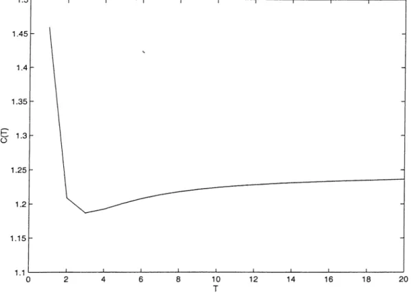
4.1 The graph of C{T) when Co = 1, Ci = 0, C2 = 0.0125, N = 100 and Л = 1... 61

(12)

List of Tables

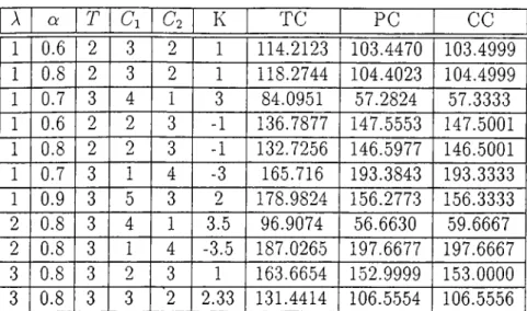
4.1 Long-run Expected Co.sts of Total Control, Partial Control and Cyclic Control for Different Values of Parameters... 67

4.2 Simulated T'* values when a = 1, (Co = 1, (Ci = 0, C2 = 0.0124867, N = 100 and A = 1. 67

4.3 Signs of f{x)· (If f{x) > 0, partial control is better than total c o n tr o l.) ... 67

(13)

Chapter 1 IN T R O D U C T IO N

Reliability ^ is design engineering discipline which applies scientific knowledge to assure a product will perform its intended function for the required duration within a given environment. This includes designing in the ability to maintain, test, and support the product throughout its total life cycle. Reliability is best described as product performance over time. This is accomplished concurrently with other design disciplines by contributing to the selection of the system architecture, materials, processes, and components -both software and hardware; followed by verifying the selections made by thorough analysis and test.

The skills and knowledge required to achieve reliable products are:

• statistical analysis

• product reliability modeling for selection of redundancy versus compo nent reliability

• trade study analysis

• reliability predictions

(14)

• worst case stress/tolerance/sigma design performance analysis • engineering based physics of failure

• failure modes/effects/criticality analysis

• reliability test planning and testing - product stress screening/accelareted life/demonstration

• failure analysis

• maintenance concept definition • maintainability analysis

• maintainability test planning and demonstration • supportability analysis

• derating analysis

• human engineering analysis

• product safety analysis

• reliability/niaintainability/system safety/quality/logistics support/human factors/software performance monitoring

• product effectiveness.

CHAPTER 1. INTRODUCTION 2

Many researches have been conducted on maintenance models for systems with stochastic failure in the last forty years. Maintenance models can be applied to a variety of areas such as military, industry, health, and the environment. Due to technological advances in recent decades, systems become more complicated and require new technologies, control policies and methodologies. Whichever the environment is under consideration, an important point is the determination of when to replace the system to guarantee that the system is used eifectivel}', efficiently and less costly and it is available whenever need arises.

(15)

CHAPTER 1. INTRODUCTION

In tlie thesis, we presented partial control policy with a multi-unit system. This model assumes that a random sample of n units is inspected at pre scheduled timesyT, j = 1,2,... and each failed item is replaced by new one with probability a. Consequently, the points of inspection are in general not renewal points and it is not possible to apply directly renewal theory. In literature, there are no known results about partial control of multi-unit models.

Since multi-unit maintenance models are much more difficult to analyze, the results of the single-unit models are used frequently (see examples in Section 1.1). In the usual block replacement policy (with single or multi-unit system), all units in the system are replaced simultaneously by new ones at prescribed times j T , j = 1,2,... Therefore, all known results about usual block replacement policy (to the best of our knowledge) are based on renewal theory.

In this study, we present three modified multi-unit block replacement policies. In all models, there are N units (items) which are subject to random failures. Each failed item is changed with probability a. Replacements are allowed only at times j T , j = 1,2,... and T > 0 is fixed. Some reliability characteristics are discussed under this setup.

The first model is a total control policy in which all units are controlled at times j T , j = 1,2,... Because of shortage of spare units, lack of money or workers, controlling all units may not be possible every time. So, we proposed a model called partial (group) control which depends on controlling a sample taken from all units of size n, {0 < n < N). The last model is a cyclic control in which all units are divided into r parties. Then, all parties are numbered from 1 to r. Party k is controlled at tim e jT , j = 1,2,... where j = k (modulus r) k — 1,2,..., r — 1 and if k is equal to zero then party r is controlled. We also introduced cyclic partial control which combines the partial and cyclic control policies. Under cyclic control policy, a random sample of m < n units are taken from party k at time j T , j = I , '2,... j = k (modulus 7·) k = 1, 2,..., r — 1 and if k is equal to zero then a random sample taken from party r is controlled. Then,

(16)

the failed units in the sample taken fro]n the part}' is replaced by probability ¡3.

The problem of multi-unit systems with general lifetimes practically is not analytically solvable. Thus, we study the exponential case. Since we replaced the failed items with good ones with a certain probability, the processes in our models are not renewal and regenerative processes. Hence, when we are studying the long-run behaviour of the number of failed items in the system and the cost functionals, we use the asymptotic results for Markov processes with discrete interference of chance.

1.1 Some Maintenance Policies and Litera

ture Review

Various maintenance policies are studied with a view toward information concerning their basic stochastic characteristics, such as the distribution of the number of failures, the expected time to in-service failure etc. Some decisions concerning replacement, repair and inspection are made in the study of maintenance policies.

Replacement decision making involves the problem of specifying a replacement policy which balances the cost of failures of a unit during operation against the cost of planned replacements. Two widely used replacement policies policies are age replacement and block replacement. Under age replacem.ent^ the system is replaced upon failure or upon reaching a specified age T whichever occurs first where T is considered as constant. Under block replacement, the system is replaced upon at failure and at times j T , j = 1,2,... (.see Barlow and Proschan [6]).

(17)

1979, Berg and Epstein [8] compared age, block and failure replacement (in which no preventive replacements are made at all) and provided a simple rule for choosing the least costly of the tree policies for any possible values of the planned replacement costs. Langberg [18] made the stochastic conrparisons of the number of failures and removals in an interval [0,s] under age and block replacement policies.

There is a large amount of literature on several maintenance models. In sequel, studies related to other maintenance actions and maintenance models are provided briefly.

Kaio and Osaki [16] studied the probabilistic characteristics of discrete and continuous lifetime distributions. Then, they applied the specific distributions to typical age and block replacements. The results are summarized in tables for the quick reference in real s3^stems.

Block replacement policy derives its name from the commonly employed practice of replacing a block or group of units in the system at prescribed times

j T , j = 1,2,... independent of the failure history of the sз^stem. However,

the studies on block replacement policy are usually single-unit, see e.g., Nakagawa [22]. He proposed new block replacement policies which convert the usual age, block, periodic and inspection models to discrete time replacement models. Other examples for single-unit block replacement policy have appeared in |4J |5) [6| ¡7) [11] |13J [14J (19) (20) |21| (27) and (28).

Some studies [4] [13] [17] have been written for optimization of replacement policies. Aven and Dekker [4] presented a general framework which covers many age and block replacement for this purpose.

Although the simple block replacement policy is simple to understand and easy to implement, the important disadvantage of this policy is that sometimes almost-new systems are replaced at prescribed replacement times j T , j = 1,2,... Many modifications have been introduced to avoid this unnecessary

(18)

waste: Allowing the system to remain inactive, replacing the failed item by a used one or less reliable one are some modifications. ?ilso for repairable systenis, two types of repair have been considered; minimcd and imperfect repair. Barlow and Hunter [5] introduced the block replacement policy with minimal repair at failure. Under minimal repair, the failed unit is repaired so that it functions again, but has the same failure rate and the same effective age as at the time of failure. Under imperfect repair, the failed unit is repaired with probability

p it is returned to the ”good-as-new” state (perfect repair), with probability q = 1 — p it is returned to the functioning state, but it is only as good as a

device of age equal to its age at failure (imperfect repair).

In 1979, Nakagawa [19] [20] studied block and age I'eplacement with imperfect repair. After introducing imperfect repair concept in [19], he presented optimum policies when preventive maintenance is imperfect. A year later, he gave a summary of imperfect preventive maintenance policies with minimal repair in [21].

Beichelt [7] proposed a generalized block replacement policy for a system with two failure modes. If the system is in mode 1, it is removed by minimal repair. If the system failure is in mode 2, it is removed by replacement.

Other studies in imperfect repair has a.ppeared in [11] and [14]. Fontenot and Proschan in [14] presented two models. In model I, they stated a modified age replacement model. At the beginning, a perfect repair is scheduled to take place at time T (a constant) a cost C2. If the device fails at a time tj prior to

T, it is repaired at a cost Ci < C2. This repair is perfect with probability p and imperfect (minimal) with probability q = 1—p. Model II is the same as model

I except in one concept: the unit is replaced (perfectly repaired) on the next failure after k — 1 successive imperfect repairs.

Shell [27] [28] studied the modified block replacement policies in detail. In his models, an operating system is periodically exchanged at times kT, k = 1,2,... independently of its failure history. After a generalization of the policy, he

(19)

CHAPTER 1. INTRODUCTION

proposed a model in which an operating s}^stem is either placed b}' a new or used one or minimall}/ repaired or remciins inactive until the next planned replacement at failure. In another policy, he introduced a modified block replacement with two variables and general random minimal cost. The cost of ¿th minimal repair at age y consists of two parts: C{y) is the age dependent random part, c,(y) is the deterministic part which depends on the age and the number of minimal repair. Thus, minimal repair cost id random. If the system fails in [(A; — 1)7", {k — \ ) T + Tq) it is either replaced by a new one or minimally

repaired, cincl if [(A; — 1)T + To^kT) it is either minimally repaired or remains

inactive until the next planned replacement.

The multi-unit maintenance models can be divided into the two main categories: ’’Preventive” a n d ’’preparedness” maintenance models (see in [12]). These models based on the knowledge of the state of systems. Preventive maintenance models assume that the state of equipment subject to stochastic failure is always known with certainty. Preparedness maintenance models also deal with equipment which fails stochastically; however, the state of equipment is assumed to be unknown unless either inspection or replacement is carried out. An additional decision related to an optimal inspection schedule must be made in these models.

Replacement models are included in the preventive maintenance models. In sequel, studies related replacement models with multi-unit system are provided. Tango [30] investigated a multi-unit system. He proposed a modified block replacement policy using less reliable items. If operating items fail in [(A; — 1)7", kT — u), they are replaced by new items, and in [(A: — 1)7" — kT),

they are replaced by less reliable items than new items. (Less reliable items should be cheaper and thus less durable than new items.) Haurie and L’ecu}'er [15] formulated a group maintenance replacement problem in continuous time for multi-component system having identical elements. Also, the numerical computation of optimal and suboptimal strategies of group preventive replacement are done for discrete time.

(20)

Due to the fact that items in a system function under the Scvme environmental conditions like temperature, humidity and vibrations, component lifetimes are generally stochastically dependent. Thus, they are also economically dependent because of doing preventive maintenance to functioning units. In [23], Ozekici discusses the effects of these dependencies on periodic replacement policies and provides useful characterizations of the optimal replacement polic}^

In 1990, Ritchken and Wilson [24] introduced (??r, T) group replacement policy which combines the m-failure and T-age policies. All items are replaced by new ones when the system is of age T, or when m failures have occurred whichever comes first.

Optimal group maintenance policies for a set of M identical machines subject to stochastic failures are considered in [3] [31]. Assaf and Shanthikumar [3] proposed a control limit policy which minimizes the expected cost per unit time over an infinite horizon when costs are incurred due to loss of production and repair only. In this model it is assumed that the number of failed machines in the system is unknown unless an inspection is carried out. Therefore, this model is an example for preparedness maintenance policy. In a part of their study, the following policy is considered: Inspection takes place every r units of time and all failed machines, if any, are repaired at each inspection epoch. Let W {t) be the average cost of this policy per unit of time. Then,

W M = Cq^ C od - + ./V(C· - (C./A))(l - ^

T

where Co is the overhead cost of repair, C\ is a cost of repair per machine and C2 is the cost of production loss for each failed machine during operation. Also, a positive cost Cq is paid every time such an inspection is performed.

In [31], Van Der Dyn Schouten and Vanneste introduced four possible states for each component: good, doubtful, preventive maintenance is due and failed. They considered two types of control policies which based on the number of doubtful components at component failure epochs. After introducing a general model with identical lifetime distributions for individual components, they

(21)

propose an approximate model in which the four possible states are identified with certain age intervals for each individual component.

Some other studies about multi-unit maintenance policies are the following: In 1992, Sheu and Griffith [29] studied multi-unit systems with dependent life- lenghts having certain multivariate distributions. Components are repaired upon failure (perfect or imperfect repair) depending on the different sources of failure. In the same year, several new results which connect the properties of block replacement policies with properties of corresponding renewal function and excess lifetimes are obtained in [26]. In [10] the concept of repair replacement is introduced by Block, Langberg and Savits. In repair replacement, items are repaired if they fail and replaced only if they survive beyond a certain fixed time from the last repair or replacement.

In [9], it is assumed that performance of M identical machines deteriorates with the operating time since the last maintenance and no random failures occur. Any machine can be taken off line for maintenance at any time, (that is, it is not a periodic inspection or a periodic replacement.) The maintenance times are independently and identically distributed. Under these assumptions, many maintenance policies are performed when the expected profit rate is maximized.

The rest of the thesis is organized as follows: In Chapter 2, after analyzing the behaviour of items in the system, we present total control, partial (group) control and cyclic control in discrete time. Some reliability characteristics are discussed. We compare partial (group) control and cyclic control when we consider the number of failed units in the system. In Chapter 3, all analysis for discrete time is done in continuous time. In Chapter 4, some cost functionals are studied and the optimal replacement interval T* is obtained. A simulation of total control policy is provided and the comparison with analytical result is given. Finally, we present our conclusion in Chapter 5.

(22)

Chapter 2 DISCRETE TIM E MODELS

In this chapter, we present modified multi-component block replacement policies in which units (items) are replaced only at prescribed discrete times r , 2 T ,.... In the first section, we will analyze the behaviour of items in the system and determine the number of failed units at time k, k = 0,1, 2,... . In

sequel sections, total control, partial (group) control and cyclic control policies for discrete time will be introduced.

2.1 Analysis of Behaviour of Items

Consider a discrete time control polic}c Suppo.se that there are N independent items each of which is in good condition at the beginning in the system. Let Qk be the number of failed items at time k, k = 1,2,.... Assume that every unit may fail independently of the failures of the other units with the probability q. Thus, the distribution of failed items is a binomial distribution. Let Bin{N,q) denote the Binomial random variable with parameters N and

q, that is, = 0 = ^ . j p'q^'~' where p = I - q and i - 0,1, 2,..., TV. In future we will use also the notion of double stochastic binomial random variable.

(23)

CHAPTER 2. DISCRETE TIME MODELS ₁₁

D efinition 2.1 If Z is some integer random variable with values {1,2,...}.

We will denote a double stochastic binomial random variable Bin{Z,o:) such that

a H \ - a Y ~ ^ P { Z ^ n ) . P{Btn{Z,a) = k ) ^ J 2 n

n > k V k

Expectation of the double stochastic binomial random variable is E[Bin{Z,a)] = aE{Z).

Then we can write the following stochastic relation between number of failed items at step k and A: + 1.

Qk+i — Qk + B i n f N — Qi;^ q). A: — 0,1,2,... (2.1.1)

In order to find the expected number of failed items at each step, we can use the following recurrent relation. If mr- = E{Qk) is the expected number of failed items at step A;, k = 0,1,2,.... For step A: + 1,

mfc+i = mk + {N - mk)q

or

m.k+1 = Nq + vikP where p = I — q. (2.1.2)

Since all units are in the good condition at the beginning, the expected number of failed items at initial step is zero, that is, m-o = 0. Then by Equation (2.1.2), we have the following,

mi = Nq. m2 — Nq + mip = Nq{l + p). m3 = Nq + 7TI2P = Nq{l + p + p'^). mk = Nq + rrik-ip = Nq{l + p + p^ + ... + p^ 1 -= N { l - p ) ^ . 1 - p

(24)

CHAPT'ER 2. DISCRETE TIME MODELS ₁₂

Therefore, we get

mk = N ( l - p ' ^ ) , ¿ = 0,1,2,... (2.1.3) As a result, we can say that number of failed items at step ¿, ^ = 0,1,2,... has binomial distribution with parameters N and 1 — for k = 0,1,2,....

If the number of failed units on the initial step is greater than zero, that is,

Qo > 0, with mean nio then the recurrent relation (2.1.2) gives the following:

mi = Nq + mop. Ш2 == Nq + mip = Nq{l + p) + p^'mo. шз = Nq + Ш2Р - Nq{l + p p ' ^ ) + p^mo. Finally, mk - Nq + mk-ip = Nq{l + p + p -h ... + p ) + p^mo = N { l - p ) \ — — +p''mo. 1 - p mk = N{1 - p^) + p^mo, ¿ = 0,1,2,... (2.1.4) When we compare Equation (2.1.3) and (2.1.4), there is an additional term containing expected number of failed units at the beginning in Equation (2.1.4).

Example:

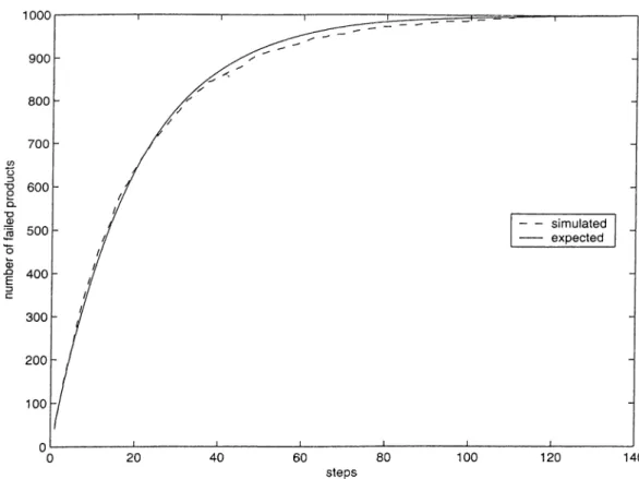
In order to demonstrate the use of the model, the case N = 1000 and q = 0.05 is analyzed. The number of failed units were obtained by simulation and the expected number of failed units for each step was calculated analytically. Since

N = 1000 and q = 0.05 the function of expected number of failed items is given

by

7Пк = 1000(1 — 0.95*") where ¿ = 0,1,2,... is any step.

At the end of 136 steps all units are failed. The graph of output is shown in Figure 2.1.

(25)

CHAPTER 2. DISCRETE TIME MODELS ₁₃

Figure 2.1: The graph of simulated and expected number of failed units for

(26)

CHAPTER 2. DISCRETE TIME MODELS 14

adding simulated binomial random variables, Qk at time k = 1,2,..., is

(27)

2.2 Total Control with Block Replacement

In this section, we study a control policy with modified block replacement. Again suppose that N independent units with failure probability q are installed. We call this control policy as “Total Control” because all installed units are controlled at time j T , j = 1,2,... where T is some positive integer. While making replacement we can make a mistake which means that we may change the failed item with good one only with probability a. We assume that replacement, repair or inspection time is negligible. Replacement is allowed only at times j T , j = 1,2,... for a fixed T > 0, that is, the failed units may be replaced only at discrete times T ,2T , ....

Consider the process at times j T , j — 1,2,... and let Qjt be the number of failed items before control at time j T , j = 1,2,... and

Mjr = E{QjT), j = l ,2,...

and let Moo be the expected number of failed items before control in the long- run, that is,

Moo = lim MjT-_{j —}_*oo

(We will prove that this limit exits.)

Main Relations:

We denote the number of failed units before control at time j T , j = 1,2,... by

QjX and the number of failed items just after control at time j T , j = 1,2,...

by Qjx- Then,

QjT — QjT — Bin{QjT,0:) (2 .2.1 )

Let

Then the expectation after control yields

Finally,

Mjy = Aljx — Mjxcx.

(28)

Rewriting Equation (2.1.1) by putting instead of Qk, we have

Q{j+i)T = QJt + Bin{N — Q'^x·, I — ) (2.2.3)

It follows that the recurrent relation for mean number of failed items is

= M/x + ( N - m;x)(i - / ) .

Substitute M^x and rewrite M(j+i)x.

M(j+i)x = (1 *- a)Mjx + (N — (1 — a)Mjx)(l — p^) = JMjx[l - a - (1 - a )(l - ; / ) ] + fV(l - p^).

M(j+i)x depending on Mjx is given by

M(j+i)x = Mjx(l - a)p^ + A^(l - p^).

In Equation (2.2.5), let a = (1 — a)p^, 0 < a < 1 and Then h = N{ \ — p^). (2.2.4) (2.2.5) — aMjT + h.

Here note that number of failed units at time 0 is greater than or equal to zero, Mo > 0. We can get M j j depending on Mo, a and 6, that is,

Mx — ciMq -j- b. M2T ~ Q·^Mq -(- cib "f b.

(29)

CHAPTER 2. DISCRETE TIME MODELS ₁₇ M.JT = MMo + a^~^b+... + ab + b = a^A4o + b J2 <i^ k=0 ( 1 - 0 ') — Mo -|- b-l — a

In general at tim ejiT, j = 1,2,...

M,T = { Mo - 7 - ^ " ) + ^

1 — a j \ — a

As the number of inspection times j goes to oo, since 0 < a < 1, then we get

lim MjT -

---j-*oo 1 — a (2.2.6)

Hence we can find average number of failed items before control in the long- run, Mco, by substituting a and b in Equation (2.2.6). Therefore,

ATI —p^)

(2-2-7) The expected number failed units just after control in the long-run is the following:

M+ = M ^ - c x M ^

= (1 - Q()Mco,

substitute Moo obtained in Equation (2.2.7) and get,

= T^(l - P )(1-a)_ .

l - ( l - a - ) p ^ ■ ^ ^

We proved that limit, as the number of inspection times j goes to infinity, exists. We can also find the limit directly from Equation (2.2.5). Thus,

lim M(j+iyr - M then.

(30)

that implies

“ 1- {1- Q y (2,2.9) In order to obtain the average long-run proportion of expected number of failures, we can use the following definitions and theorems:

D efinition 2.2 I f the random variable ^ ao, then we can denote it as

P lim (n = ao_n—₊₀₀

P

where —> denotes converges'in probability and P lim means a limit in probability.

D efinition 2.3 R(N^T^p^a) is the average long-run proportion of expected

number of failed items in the system and it is represented as follows: R { N , T , p , a ) = lim j ^ E Q u

-D efin itio n 2.4 Q{N,T,p^a) is the long-run average proportion of failed items

in the system and given by

0 ( A '.r ,p ,a ) = F lim n—♦•CO 77 ^

-k = l

L em m a 2.1 The limit of the expected value of j = 0, 1 and / = 0,1,... exists and is given by

where

lim EQiT+j = EJ"' /—♦CO

E r = M * + { N - y )(1 - p>).

Proof:

EQiT+j can be expressed by using Equation (2.1.3) as EQiT+, = MS- + ( N - M t r ) { l - p ’ )

(31)

CHAPTER 2. DISCRETE TIME MODELS ₁₉

where M ^ is the expected number of failed items just after control at time IT^

I = 0,1,... Therefore, as / ^ oo, we ha.ve

lirn EQ,T+, = M+ + {N - M+){1 - jA).

i—*-oo □

L em m a 2.2 If Uk as k —* oo then, 1 ”

— 7 aic a<x, as n —> oo.

Proof:

2 ^ \ ^ 2 ^

I ^ ^ ôo| ^ y 1^/: ôo I — ^ V l^/c ôo| "I" ^ ^ |^/c

/:=! /c=l /c=l k=l ^ ^-= L + l

n

< e - = e,

n

As ak goes to aco, then for any e > 0, there exists L such that k >

\dk “ <^co| < ^7 then

1 ^

> U q q. □

T h eo re m 2.1 Let EQk be the expected number of failed units at time k, k

1,2,.... The7i, we have

R[N, T, p. a) = lim i E e T “

"■ k=\ j=0

where Ef° is obtained by stochastic relation (2.2.5) in the long-run, that is, E T = W t + (.'V - M i) ( l - f ) ] ·

Proof:

If n =z T m , ^ Y fk = \ ^ Q k can be written in the following form: 1 / 1 m 1 77i 1 m ''

(32)

Consider EQiT+j for 0 < j < T, and refer to Lemma 2.1. As / —> oo, we get

EQI T+j ET.

Using Lemma 2.2 we get for an}^ j as rn —> oo, 1

m T.E Q_l=l 41T+İ ET.

where

E f = [M+ + (A' - W+)(l - P’ )].

M ^ is the average long-run number of failed items just after control and {N —

— pf) is average number of items failed during time (ITCT + j) in the long-run. Consider the case n = Tm-\-i where 0 < i < T. ^ EQk can be

written in the following form:

1 ( m m m \ Tm-\-i

'ÊQtr t YÊQit+1 + ■■■+ 'ÊQiT+T-ij + EQj

1=1 1=1 1=1 J j= T m

T m i

Rewrite the equation then we get

'T 'm \ ^ ^ 1 m 1 m ^ EQljr H---- EQiT-\-i + ... H---Y2 ^Ç/T+T-1 T m + i j T \ m m ₁₌₁ m ₁₌₁ T m + i

- E EQi

Note that 1 Tm+i jyf· T m + i

As m goes to infinity, the term (2.2.10) goes to zero and

T m ^

T m + i

Therefore, we get the same situation when the case n = Tm.

(2.2.10)

□

Theorem 2.2 In the long-run, average proportion of number of failed units Q ( N , T , p , a ) exists and it is given by

1

Q{N,T,p,a) = ~ J2 E·

(33)

Proof:

Let us represent the value 1/n Qk hi the following way: Consider at fixed j = 0,1,..., T - 1 a sequence Qir+j, I - 0,1,... and the case when n = Trn, then

■in i / - j m - j m -1771 \

- E = 7^ ( — £

QlT

+ — £

QiT+i

+ ··· + — S

QlT+r-1

I

n T \ m ₁₌₁ ₁₌₁

It can be easily see that this sequence Qir+j, I = 0,1,... forms a Markov process which is embedded for Qk- Lets find a limit of the value l / n ^ ¿ _ j Qk- Consider first the sequence Qit, I = 0,1,... This sequence forms an irreducible Markov chain with finite state space {0,1,..., N} and corresponding transition probabilities p,j, i j = 0 ,1 ,...,//. Denote for any i — 0 ,1 ,...,//

C' = « -f B in { N — C l — P^) * = O51) ···//·

Then, transition probabilities are obtained by

Vгi = P[C = i) > 0 C j = 0,1, ...Ah

Let 7r(f), i = 0,1,..., / / denote the stationary distribution of the Markov chain

Q i T - According to weak la,w of large numbers for Markov chain, as m —> 0 0,

we get

1 “

m _/=1

where

Now let us show .that

Remember that N ¿=0 E , Q * = M+. — lim EQ lj· k—^oo

Let be the expected number of failed items just after control at time ¿T,

k = 1,2,.... Hence,

v * = EQt^r = ¿=1

(34)

CHAPTER 2. DISCRETE TIME MODELS 99.

where PkT{^) — P{Qk:r — 0· QkT is ergodic Markov chain then as k —> oo,

P k r { i ) T ^ { i ) ¿ = 0 ,1 ,...,Ah Thus, we have

= iiiTi EQl^r = ¿ * 7t(z) = E^Q"^

k—*oo _{i = l}

In the same wa.y, we can prove that each j = 1,2,..., T - 1, Qtx+j forms an ergodic Markov chain and

m ^ QiT+j E] 7100 'j 1=1 Finally we get. 1 T-i Q ( N , T , p , a ) = - Y , E ^ ^ k=0

Similarly as in Theorem 2.1 the case when n = Tm + ¿, 0 < i < T is the same as the case n = Tm. □

Corollary 2.1 The average long-run proportion of failed items in the system is equal to the average long-run proportion of expected number of failed items in the system. That is,

Q { N , r , p , a ) = R ( N , T , p , a )

Proof;

It is obviously follows from Theorem 2.1 and Theorem 2.2. □

Corollary 2.2 The average long-run proportion of average number of failed items for total control in the system is the following:

\ /1 — ' iг(A^Γ,p,αO = ¿V 1 - 4

a

T \ l — {1 — a)p'^J \ 1 — p (2.2.11)

Proof:

Proof of this theorem based on Theorem 2.1.

1 r - i

i?(A^Γ,p,α) = jim - ^ EQ^_n—_{*oo 72} t - ^ ~ ^ 0 ( 1 " P )]·

(35)

CHAPTER 2. DISCRETE TIME MODELS 23 Equivalently, 1 r - l R ( N , T , p , a ) = + k=0 T-1 k=0 k=0 = N - ^ ( N - M ^ ) f : p'' k=0 T _k=0 1

substitute obtained at Equation (2.2.8), then

R ( N M = = TV 1 - Finally we have, R ( N , T , p , a ) = N 1 - p J 1 f 1 — p^ + ap^ — I -\- a p^ — ap^ T

1 - 1

1 — (1 — a)p^ a \ f I — p^ T \ 1 — (1 — a)p'^

J

\ I — p . 1 - P

(36)

2.3 Partial (Group) Control with Block Re

placement

In practical models it is difficult to inspect all units at the control times JT,

j = 1,2,... when the number of installed units are large at the beginning.

Control of all operating units requires a large amount of spare units, money and workers. In order to avoid high cost, in this section, we will introduce a modified block replacement which depends on control of a partial choice of whole units in the .system.

Assume that there are N units in the system. Each item ma.y fail with probability q. At each control time jT , j = 1,2,... we take a sample of size n where n < N units are selected randomly from the all units in the system. Assume that the probability of changing the failed unit with a good one in the sample is ¡5. Let QjT be the total number of failed items at time j T ,

j = 1,2,... and (5/r number of failed products just after control. The sample contains HG{N,n,QjT) faulty units at the inspection time, where

HG{N,n,QjT) is a double stochastic hypergeometric random variable with

parameters N , n and QjT, th3,t is.

N - QjT n - k

P{HG{N,n,Q,T) = k} =

where A: = 0,1,2, ...,n and E{R ) = n{MjTlN)

(Inspection technique is based on the model of Anisimov and Sereda [1].)

Suppose that MjT = E{QjT) and = ^(Q^t)· The following stochastic

relation contains again a double stochastic binomial random variable as explained in Definition 1.1. Then, we get

(37)

CHAPTER 2. DISCRETE TIME MODELS ₂₅

If we take the expectation of both sides in Equation (2.3.1), then we have

(2.3.2)

If we consider the number of failed items at time {j + 1)T then,

MIt = M,T - M j T ^ 0 = ( ^ 1 - ^ 0 ) M,T.

Q[j+i)T — Q'jT + Bin{N — Q/t) ^ ~ P ) (2.3.3) The stochastic relation between the avera.ge number of failed items before control at time [j + 1)T and and the average number of failed units just after control at time , j T is the following:

n

= MjT (1 - ) p‘ ' + yvil - p’ ’). (2.3.4)

C o ro llary 2.3 Consider the partial (group) control with block replacement.

The long-run average number of failed items before control in the system is given by where Jim MjT = Mooi *-00 _ i v ( i - p q 1 - ( ] - / ? § )p^·

The expected number of failed units just after control in the long-run is the following:

< = (1 - /* ^ 1

substitute Moo then,

, , , _ N { l - p n { l - 0 j , )

(38)

The average long-run proportion of number of failed products is the following:

R { N , T , p , n , ^ ) = N 1 - 4

0— 1—

p^

T

V i - p

(2.3.5)

Proof:

Equation (2.3.4) is basic stochastic relation for partial control to obtain the long-run values given the theorem. When we compare the Equation (2.3.4) with Equation (2.2..5) which is basic for total control, ct is replaced by /3nfN. So, in Equations (2.2.2) and (2.2.7), a is replaced by the probability /3{nlN) and get analogous results for this model. □

Example:

If all failed units in the sample are changed with good ones, that is, /9 = 1, we have

QlT = Q j T - H G { N , n , Q , T )

taking expectation of both sides yields.

The stochastic relation between the time jT and (j + l ) T is

Q(j+i)T = Q~jT + — Q^Ti ^ ~ P^) and

(39)

CHAPTER 2. DISCRETE TIME MODELS ₂₇

2.4 Cyclic Control with Block Replacement

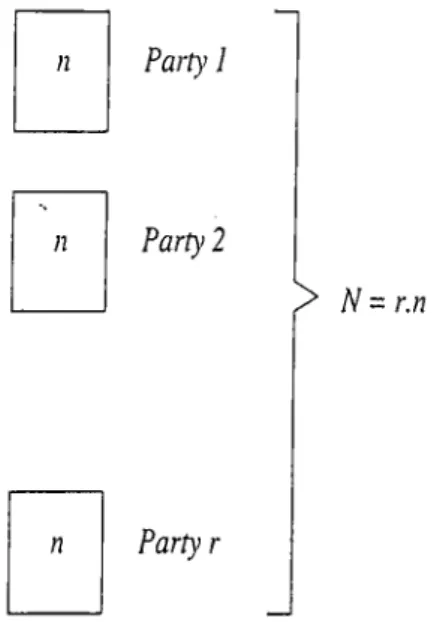
In the previous model, the sample chosen for the control was selected randomly. In this model, we assume that N installed units are divided into fixed r groups (parties) each of which has n independent items (that is, N = nr). Figure 2.2 shows the partition of N items. Each item in the system may fail with

P a r ty 1

P a r ty 2

> N = r.n

P a r ty r

Figure 2.2: The partition of N units.

probability q in each step. Let j T , j = 1,2,... be the control times. Party 1 is controlled at time T, party 2 is controlled at time 2T, party 3 is controlled at time 3T, this continues until inspection of party r at time rT. The first “cycle of control” is completed when party 1 is controlled again at time (r + and is equal to rT. Then, the second control cycle begins. Note that all units are inspected in party k, k — 1,2, ...,r. Figure 2.3 summarizes the control times of parties. We change the failed unit with good one with probability q· only

--- ^ ^ ^ ^ ^ ^ ^ ^ T

t

2T

t

3T

f

(r-I)T

t

rT

f

(r+I)T

f

(r+2)T.

t

1 Control 1

Control Control1 Control1

1

Control Control1 Control1 Party J Party 2 Party 3 Party (r-I) Party r Party J Party 2

(40)

CHAPTER 2. DISCRETE TIME MODELS ₂₈

at times jT^ j — 1,2,... lor a fixed T > 0. In this model we assume that replacement, repair or inspection time is negligible.

Before starting calculations, let us introduce the notation used. For j — 1,2,...,

k = 1,2,..., r and fixed T > 0: Notation

M^'^ expected number of failed units for party k at time [k — \)T. q probability of failure for each item on each step.

r number of parties in the system, n total number of items in party k.

a probability of changing the failed unit with a a good one at time control j T . Under assumption that all items are in the good condition at time 0, expected number of failed units for party k at time [k — l)?^. We get the following relations:

= 0

=

n (l - / ) n (l

-If we know the average number of failed units for party 1 at any time jT , (U

j = 1,2,... we can easily calculate that for other parties by changing M^0 > k = 2,3,4,... with Mq\ Note that kT^ {r + k)T, (2r + k)T, ..., (/r + k)T are

the control times of party k, k — l,2 ,...,r .

C orollary 2.4 Consider the cyclic control with block replacement. The long-

run average number of failed units before control is the following,

amd the average number of failed items jtist after control, M+ = (1 - a ) M ^ .

(41)

The average long-run proportion of expected number of failed units is given by

(2.4.1) p^^'{l — Ci)) \ I — P

Proof:

In cyclic control we divide the items into r different parties each of which has n items. Cyclic control can be thought as r different total control models having n units with operation time interval rT. So, if we put n and rT instead of N and r , respectively, in the formulae of total control, we obtain the formulae for only one party of cyclic control. That is.

n{l — Q')(l — 1 — (1 — a )p,rT and R{N,rT,p,n,(y) = n ₁ - ^1 a ' I - p xT' rT \1 — — oi)) y 1 — p

Since there are r parties in the system, we multiply M ^ and R{ N^rT,p,n,a) by r to obtain final the formulae for the system. □

(42)

CHAPTER 2. DISCRETE TIME MODELS ₃₀

2.5 Comparison of Partial (Group) Control

and Cyclic Control

In previous sections some discrete time control models are introduced. As we stated before, in both partial (group) control and cyclic control we control n units of the system at prescribed control times j l \ j — 1,2,.... A question may arise:

Which model is better if we consider the average number of failed units?

In order to answer this question average long run proportions of expected number failed items can be used. Recall Equations (2.3.5) and (2.4.1) under the assumption that all parameters N, T, p and n are the same for both models and probability of changing failed unit with good one /? and a are equal to each other for partial choice control and cyclic control, respectively:

Partial (Group) Control

R{N^ T,p^ 77,, a) = N ₁ - 7^1 T U - ( l - c r ^ ) p ^ 1 - / , 1 - p Cyclic control ■R{N,rT,p,n,o) = ^ - ^ ( i _ p ” i _ ^ ) ) ( V r 7 ) \ / 1 = N I - i T \ l — P''^(l — ce)

J

\ I — P

Now we claim that the average number of failed units for “Cyclic Control” is less than the average number of failed units for “Partial Control” a.t any time.

If we examine Equations (2.3.5) and (2.4.1), it is enough to check the following inequality.

(43)

CHAPTER 2. DISCRETE TIME MODELS ₃₁

an a?i

T \ l - ^'■'^(1 - a)

J

\ I - p

J

~ T \ l - {I - a^)p'^

J

\ I - p J

As defined before N is equal to rn so we may put 1/r instead of n/A^ After cancellations, previous inequality yields,

1 - p tT

> 1 - p T

1 — p'^'^(l — O') 1 — (1 — afr)p^ equivalently.

(1 - p"^)[l - (1 - aVr)?/] > (1 - p^)[l - ? /^ (l - a)] after making some cancellations,

T „ ( r + l ) T

--->prT_p{r+l)T

r r

Let put terms on the right to the left and denote this function f { T )

T „ ( r + l ) T

f { T ) = ? - - ^--- p'·^ + ph+i)i'·

r r

Thus, if our claim is true, f { T ) > 0 should be satisfied.

T h e o re m 2.3 If a ^ [0,1] and for any p € [0,1], fixed T > 0, n < N where

N = 1,2,... and r = N / n , then,

rR(N, rT, p, ?7.) < R{N, r , p, n) (2.5.1)

that means the average long-run proportion of failed items for cyclic control is less than the average long-run proportion of failed items for partial (group) control.

Proof:

Consider the function f { T )

P^ + r I ilT

f(T) i---p’·^ + r r

To show f { T ) > 0 we may take derivative with respect to T and check whether it is greater than 0, that is, f ' ( T ) > 0. However, it is not visible to show in

(44)

this way. So, let

X = p

where 0 < p < 1 and T > 0, then 0 < x < 1. Function depending on x will be the following:

h(x) = ---- x’’ + ( l ---1

it yields,

h{x) = —[1 — + x’’(r — 1)] r

where x /r is always positive since 0 < x < 1 and r = 2 ,3,4,.... Now let

h{x) = (x/r)g{x)

g{x) = 1 — rx ’’“ ^ + x’’(r — 1)

Note that on boundary points of x, p(0) = 1 and p(l) = 0. Also, g{x) is continuous on [0,1]. Thus,

g'(x) = r(r — l)x ’’ r( r —1)Xr - 2

— r( r — l)x '‘ ^(x — 1)

Since r(r — l)x ''“^ > 0 and (x — 1) < 0, this means that g'{x) is less than zero. We can conclude that g{x) is strictly decreasing function on [0,1]. Therefore,

I € (0,1)’S ’ [0.1]

Since 0 < g{x) < 1 for every x € [0,1], in conclusion, we can say that h{x) > 0, X G (0,1). Therefore our claim that the average number of failed items in “Cyclic Control” is less than or equal to the average number of failed items in “Partial Control” is true. Note that if 0 < p < 1, we have strict inequality in

(45)

Chapter 3 C O N TIN U O U S T IM E

M ODELS

In this chapter some modified replacement policies will be studied with multi- component units in continuous time. We will consider their basic stochastic characteristics, such as the number of failed items at any replacement time

j T ^ j = 1,2,..., where T is fixed, its mean value and long-run proportion.

In the first section, we will construct a model without rei^lacement in order to determine the number of failed units at an}^ time t , t > 0. In the second section, total control with periodic replacement will be studied. In this model, all failed units are replaced with good ones at time jT,,;' = 1,2,.... In sequel sections, partial choice control and cyclic control will be discussed for continuous time.

3.1 A Continuous Time Model without Re

placement

In this section, we construct a model which constitutes the core of our replacement models in the succeeding sections. N identical units are installed at the beginning. Each unit in the system is assumed to fail with rate A.

(46)

CHAPTER 3. CONTINUOUS TIME MODELS 34

Let Q{t) denote the number of failed items at time t. Suppose that Q(0) =

Qo and let

m{t) = E[Q{t)]

we will determine m{t) deriving and then solving a differential equation.

We start by deriving an equation for 7n{t + h) by conditioning on Q{t). This yields

m{t + h) = E[Q{t + h)] = E[E[Q{t + /i)|g(f)]]

Now, given the size of the system at time t then, ignoring events whose probability o(/i), the system at time t P h will increase in size 1 if a failure occurs in (i, t + h) or remain the same if no failures occurs. That is, given Q{t)

Q{t + /?.) —

Therefore,

Q[t) with probability 1 — \ { N — Q{t))h + o{h)

Q{t) + 1 with probability X{N — Q{t))h + o{h)

E[Q{t + h)\Q(t)] = Q{t) + \ { N - Q{t))h + o{h)

Taking expectations yields

or equivalently

m.{t + h) = m{t) + A(jV — m{t))h + o{h)

m(t + h ) - n ^ ^ 0(h)

h '■ ' h

Taking the limit as h 0 yields the differential equation

m (t) = \ { N — 7n{t)) (3 .U ) then Integration yields = A. A[A^ — m{t)] -ln[X{N - m(f))] = Ai + c

(47)

CHAPTER 3. CONTINUO US TIME MODELS ₃₅

Therefore,

X(N - m(i)) = Ke-Xt 7Tl{t) = N

A

To determine the value of the constant we use the fact that ?7z(0) = mo and evaluate the preceding at t = 0.

This gives

\ { N - 77lo) = K

Substituting this back in the preceding equation for m{t) yields the following

m{t) = N — (N — rno)e~^^

If the number of failed products at the beginning is zero, that is, (^(O) = 0, then its expectation will be m(0) = 0. Therefore, we get

m{t) = N{1 — e i > 0 (3.1.2)

When we compare Equation (3.1.2) with Equation (2.1.3), for discrete timep*" is changed with for continuous case. In conclusion, the number of failed units at time i, t > 0 has binomial distribution with parameters N and 1 — for t > 0.

(48)

CHA PTER 3. CON TIN UO US TIME MODELS ₃₆

3.2 Total Control with Block Replacement

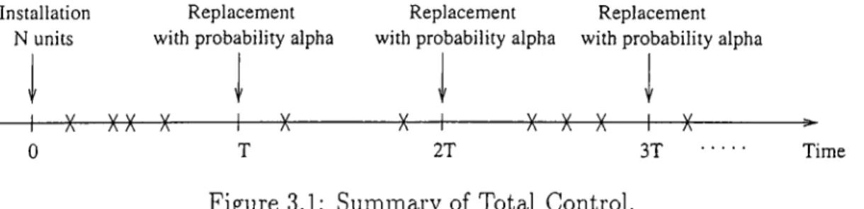
In this section we consider multi-component total control with periodic replacement for continuous time. At time zero N units are in the good condition. After a fixed time period T, the replacement of some units are made with probability a. That is, while making replacement we make mistake with probability I — a. Total control is different from the block replacement in such a way that replacements are allowed only at times j T , j — 1,2,... where T is a positive real value. Figure 3.1 summarizes total control. Marks between control times j T and {j + 1)2' represent the failures.

Unlike block replacement, total control cannot be represented as a renewal Installation

N units

-3— X— 0

Replacement with probability alpha

Replacement Replacement with probability alpha with probability alpha

+ ---l· --X X— ^—

X-T 2T 3T

Figure 3.1: Summary of Total Control.

Time

process because of making mistake in replacements at control times. We assume that replacement, repair or inspection are made immediately.

Before starting to calculate some stochastic characteristics of this model, we will define the notation. Note that the following notation will be used for all other continuous time models in this chapter.

Notation:

For j = 1,2,...,

N total number of items in the system.

a probability of changing the failed unit with good one. A intensity of failure of each item.

Q{jT) number of failed items in the system at time j T before control.

M { j T ) expected number of failed units in the system at time j T before control.

(49)

CHAPTER 3. CONTINUO US TIME MODELS 37

yV/+(jT) expected number of failed units in the system just after control at time j T .

C o ro lla ry 3.1 Consider the total control policy in continuous time. The recxLrrent relation for the number of failed items is given by

Q[{j + l) r ] =

g+(;T)

+ B m { N -

g+(jT),

1 - e (3.2.1)

where B in { N — Q~^{jT), 1 — denotes the number of failed products during operation time { j T ,( j + 1)T), j — 1,2,.... And the recurrent relation for average mimber of failed items by using expected value of Equation (3.2.1) is the following,

M[{j + l ) r ] = (1 - a ) e - ^ ^ M { jT ) + N{1 - ) (3.2.2)

P roof:

Since there is a one to one correspondence between discrete time and continuous time, we simply put instead of p^ in Equations (2.2.3) and (2.2.5).

□

C o ro llary 3.2 The long-run average number of failed items before control for

total control is the following:

N { l - e - ^ ^ )

1 - (1 - a)e-^T (3.2.3)

and the average number of faulty units in the system just after control is given by

M+ = ( l - a ) M ^ .

P roof:

We know that the limits exist when the number of inspection times goes to infinity. In Equation (3.2.2) j goes to infinity, we have

(50)

And then we get the final average long-run equation. Since we change the failed item with good one with probabilit}^ a-, we have (1 — a ) M ^ failed items just after control. □

T h e o re m 3.1 The average long-run proportion of the average number of failed

items is given by

^ [m; + (iV - M i ) ( l - e-^·)] dt T Jo

as t oo.

P ro o f:

The average proportion of number of failed items at time t is the following: 1 U

- I ElQ(t)]dt

L· <J 0

and when t = n T we can write it in the following form:

1 ” 1 r(k+i)T

n f JkT {E[Q(kT)+] + { N - E[Q{kTy]){l - e-"“)} du.

As n goes to oo, then t goes to oo. Now we can use Lemma 2.2 and take into account that as A: —+ oo,

E[Q{kT)*] ^ M*.

Then as i —> oo, we have

i f B{Q{t)]dt (M i + (Ai - M i)(l - du.

The case when t — n T i, i < T is similar to the situation in Theorem 2.1.

Therefore, it is the same with the case t = n T in the long-run. □

C o ro llary 3.3 The average log-run proportion of failed units in the system for

total control is obtained as

R{N,T,X,a) = N 1 - ^1

a 1

t

(1

(51)

CHAPTER 3. CONTINUO US TIME MODELS ₃₉

P roof:

By Theorem 3.1 the average long-run proportion of the average number of failed items can be calculated using average number of faulty units just after control in the long-run.

1 T

R ( N , T , \ , a ) = - j f [m£ + (Ai - 0 ( 1 - e -« ) dt 1 t=T

t +

¿=0

After taking integration,

,-AT ₁

R ( N , T , X , a ) = V + + i ( l V o i r + ^

-Substitute M ^ in the long-run equation. Then we get,

R { N ,T ,X , a ) = 7V -

Rewrite the equation,

N - N{1 - - a) 1 - (1 - a)e-^^ J XT^ ( 1 -R { N , T , X ,a ) = N - N = N 1 — (1 — — ^') 1 — (1 — a')e”^^ a \ 1 (1 -Vl - (1 -Q )e -^ ^ y XT

Then we get the final formula for the long-run proportion. □

R em ark :

Note that the average long-run proportion of expected number of failed items for discrete time and that for continuous time are different, [See Equations (2.2.11) and (3.2.4)].

(52)

3.3 Partial (Group) Control with Block Re

placement

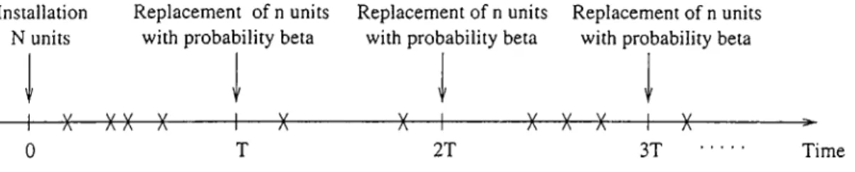
In this section a multi-component modified block replacement policy is introduced for continuous time. Assume that there are N components in the system and each unit may fail with intensity A. At time j T where j — 1,2,... we take a random sample of size n, n < N and then replace faulty units with probability Figure 3.2 shows the summary of partial (group) control. Remark that this model also cannot be represented as a renewal process.

Installation Replacement of n units Replacement of n units Replacement of n units N units with probability beta with probability beta with probability beta

H— )(— ^---- )(- X X X ----^—

X-0 T 2T 3T

Figure 3.2; Summary of Partial (Group) Control.

Time

Additional notation which we will use:

n size of random sample taken from N units.

¡3 probability of changing failed item with good one.

C o ro llary 3.4 Suppose that Q{jT) is the number of failed units at time j T ,

j = 1,2,... with expectation M { j T ) for partial control. The number of failed units just after control is given by

QHjT) = QUT) - B m {H G \N .n.Q {]T)U i} after taking expectations of both sides,

M * ( ] T ) = M { j T ) - ^ 0 M ( 3 T )

= (i - F'’)

The recurrent relation is given by

Modified block replacement models in discrete and continuous time