Attributed Relational Graphs for Cell Nucleus
Segmentation in Fluorescence Microscopy Images
Salim Arslan, Student Member, IEEE, Tulin Ersahin, Rengul Cetin-Atalay, and
Cigdem Gunduz-Demir*, Member, IEEE
Abstract—More rapid and accurate high-throughput screening
in molecular cellular biology research has become possible with the development of automated microscopy imaging, for which cell nucleus segmentation commonly constitutes the core step. Al-though several promising methods exist for segmenting the nuclei of monolayer isolated and less-confluent cells, it still remains an open problem to segment the nuclei of more-confluent cells, which tend to grow in overlayers. To address this problem, we propose a new model-based nucleus segmentation algorithm. This algorithm models how a human locates a nucleus by identifying the nucleus boundaries and piecing them together. In this algorithm, we define four types of primitives to represent nucleus boundaries at different orientations and construct an attributed relational graph on the primitives to represent their spatial relations. Then, we reduce the nucleus identification problem to finding predefined structural patterns in the constructed graph and also use the primitives in region growing to delineate the nucleus borders. Working with fluorescence microscopy images, our experiments demonstrate that the proposed algorithm identifies nuclei better than previous nucleus segmentation algorithms.
Index Terms—Attributed relational graph, fluorescence
mi-croscopy imaging, graph, model-based segmentation, nucleus segmentation.
I. INTRODUCTION
A
UTOMATED fluorescence microscopy imaging systems are becoming important tools for molecular cellular biology research because they enable rapid high-throughput screening with better reproducibility. The first step of these systems typically includes cell/nucleus segmentation, which greatly affects the success of the other system steps. These systems can be used in different types of biological applications for cells showing different characteristics. Many types of cells grow as monolayer isolated cells, whereas some grow in over-layers on top of each other. These overlayered cells (also calledManuscript received January 17, 2013; revised March 12, 2013; accepted March 20, 2013. Date of publication March 28, 2013; date of current version May 29, 2013. This work was funded by the Scientific and Technological Re-search Council of Turkey under Project TÜBİTAK109E206. Asterisk indicates
corresponding author.
S. Arslan is with the Department of Computer Engineering, Bilkent Univer-sity, TR-06800 Ankara, Turkey (e-mail: [email protected]).
T. Ersahin and R. Cetin-Atalay are with the Department of Molecular Bi-ology and Genetics, Bilkent University, TR-06800 Ankara, Turkey (e-mail: [email protected]; [email protected]).
*C. Gunduz-Demir is with the Department of Computer Engineering, Bilkent University, TR-06800 Ankara, Turkey (e-mail: [email protected]).
Color versions of one or more of the figures in this paper are available online at http://ieeexplore.ieee.org.
Digital Object Identifier 10.1109/TMI.2013.2255309
cell clumps) take up more space, which makes them more con-fluent. A high occlusion level in cell clumps decreases contrast among the nuclei, which makes their boundaries more difficult to perceive. This, in turn, may result in identifying multiple nuclei as a single cluster or identifying a single nucleus as fragments. Moreover, nonideal experimental conditions, such as weak staining and poor background illumination, may lead to nucleus misidentification. Thus, it is of great importance to develop segmentation algorithms that are robust to nonideal conditions and can operate on the nuclei of isolated and over-layered cells.
Several studies on cell nucleus segmentation exist in the liter-ature. When images comprise monolayer isolated or less-over-layered cells, relatively simple methods such as thresholding [1] and clustering [2] can be used. These methods, however, are typ-ically inadequate for segmenting the nuclei of more-overlayered cells. In such cases, the most commonly used methods include marker-controlled watersheds and model-based segmentation algorithms. The former usually define a set of markers through pixel intensities/gradients [3] and/or distance transforms [4], [5], and let water rise only from these markers. These methods usually apply a merging process [6] on their results to overcome the over-segmentation problem, which is typically observed in watersheds. Model-based segmentation uses a priori informa-tion on nucleus properties to decompose overlayered nuclei. Ex-amples include using roundness and convexity properties of a nucleus [7], [8] and a symmetry property of its boundaries [9]. Although all these methods lead to promising results, challenges still remain in segmenting the nuclei of overlayered cells be-cause of the nature of the problem. Nucleus segmentation, like all other segmentation problems, heavily depends on the seg-menter’s abilities to differentiate between noise and nuclei, dis-cern image variations, and decompose overlayered nuclei.
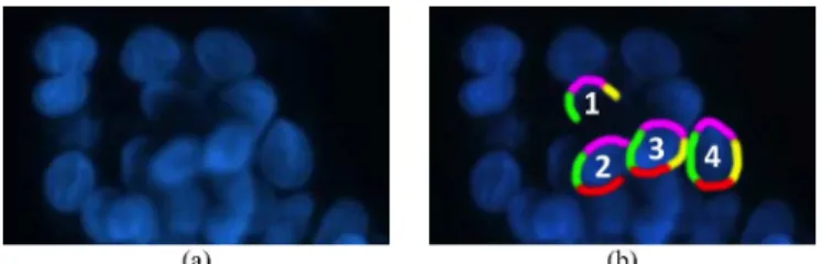
In this paper, we introduce a new model-based nucleus seg-mentation algorithm, which relies on a trivial fact that each nu-cleus has a left boundary, a right boundary, a top boundary, and a bottom boundary, and these boundaries must be in the cor-rect positions in relation to each other. Fig. 1 illustrates these boundaries for four nuclei with the left, right, top, and bottom boundaries shown as green, yellow, pink, and red, respectively. In the figure, one can observe that the bottom (red) boundary of Nucleus 1 is not identified due to an uneven lighting condi-tion. Similarly, the right (yellow) boundary of Nucleus 2 is not present in the image due to its partial overlapping with Nucleus 3. However, it is possible to identify these two nuclei by using only the present boundaries and their spatial relations. More-over, here it is obvious that the green boundary of Nucleus 3
Fig. 1. (a) An image of HepG2 hepatocellular carcinoma cell nuclei. (b) For four individual nuclei, the left, right, top, and bottom boundaries are shown as green, yellow, pink, and red, respectively.
cannot belong to Nucleus 2, and we can see that Nucleus 3 over-laps with Nucleus 2. On the other hand, the boundaries of Nu-cleus 3 and NuNu-cleus 4 form closed shapes, making them easy to separate from the background. In this work, such observations are our main motivations behind implementing the proposed al-gorithm.
Our contributions are threefold. First, we represent nucleus boundaries at different orientations (left, right, top, and bottom) by defining four types of primitives and construct an attributed relational graph on these primitives to represent their spatial re-lations (we call our algorithm ARGraphs). Second, we reduce the nucleus identification problem to locating predefined struc-tural patterns on the constructed graph. Third, we employ the boundary primitives in region growing to delineate the nucleus borders. The proposed algorithm mainly differs from previous nucleus segmentation algorithms in the following aspect: In-stead of directly working on image pixels, our algorithm works on high-level boundary primitives that better correlate with the image semantics. Using boundary primitives better decomposes overlayered nuclei and this method is generally less vulnerable to the noise and variations typically observed at the pixel level. The proposed algorithm differs from previous model-based seg-mentation methods by attributing boundary primitives to a type and locating nuclei via searching for structural patterns on a re-lated graph constructed on the attributed primitives. Working on 2661 nuclei, our experiments demonstrate that the proposed algorithm improves the segmentation performance of fluores-cence microscopy images compared to its counterparts.
II. RELATEDWORK
Many studies have been proposed for nucleus segmentation. Simple methods are usually sufficient to segment the nuclei of monolayer isolated cells; for example, one can obtain a binary map by thresholding [1], clustering [2], [10], or classification [11] and find connected components of this map to locate the nuclei. It is possible to refine boundaries using active contour models, which converge to final boundaries by minimizing the energy functions usually defined on intensities/gradients and contour curvatures [12]–[14].
To segment the nuclei of overlayered cells, however, it is necessary to decompose clusters into separate nuclei. There are two classes of methods commonly used for this purpose: marker-controlled watersheds and model-based segmentation algorithms. The former use predefined markers (which will correspond to nucleus locations) as regional minima and start a flooding process only from these markers. With this method, it
is crucial to correctly determine the markers, and one way of doing that is to select local minima on pixel intensities/gradi-ents [3], [6] and/or distance transforms [5], [15]. Another way is to iteratively apply morphological erosion on nuclear regions of the binary map [16], [17]. Because these methods usually yield more markers than the actual cells, it is common to use the h-minima transform to suppress undesired minima [4], [18]. Many studies postprocess the segmented nuclei obtained by these watersheds because they often yield over-segmentation. This postprocessing is based on features extracted from the segmented nuclei and boundaries of adjacent ones. To merge the over-segmented nuclei, the extracted features are subjected to rule-based techniques [19], [20], recursive algorithms [6], [21], and statistical models learned from training samples [22], [23].
Model-based segmentation algorithms decompose overlay-ered nucleus clusters into separate nuclei by constructing a model on a priori information about nucleus properties. A large set of these algorithms uses a nucleus’ convexity property. Thus, they locate concave points, which correspond to places where two nuclei meet, on cluster boundaries and decompose the clusters from these points. They typically use curvature analysis [24], [25] to find the concave points but points can also be found by identifying pixels farthest from the convex hull of the clusters [8]. The studies use different methods, such as Delaunay triangulation [25], ellipse-fitting [26], and path-following [27], to decompose the cluster from the concave points. Another set of models uses a radial-symmetry property of nucleus boundaries. They locate nucleus centers by having pixels iteratively vote at a given radius and orientation spec-ified by the predefined kernels [9], [28], [29]. One can also use radial-symmetry points in a rule-based method to find the splitting points [30]. A smaller set of models exists that uses the roundness property of a nucleus. These locate circles/ellipses on nuclear regions of the binary map to find initial boundaries and refine them afterwards [7], [31].
There are other classes of methods for nucleus segmenta-tion. One uses filters that have been defined considering nu-cleus’ roundness and convexity properties. Using the responses obtained from these filters, pixels with high responses are se-lected as initial nucleus locations. These locations are further processed to determine the nucleus borders [32], [33]. Another class uses density functions to locate nuclei on images. Studies use supervised [34] and unsupervised methods [35] to learn these functions.
III. METHODOLOGY
The proposed algorithm relies on modeling cell nucleus boundaries for segmentation. We approximately represent the boundaries by defining high-level primitives and use them in two main steps: 1) nucleus identification and 2) region-growing. In the first step, we construct a graph on the primitives ac-cording to their types and adjacency. Then, we use an iterative search algorithm that locates predefined structural patterns on the graph and identifies the located structures as nuclei if they satisfy the shape constraints. The region-growing step employs the primitives to find the nucleus borders and determines the
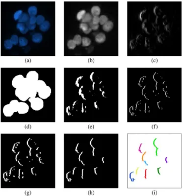
Fig. 2. Defining left boundary primitives: (a) original subimage, (b) blue band of the image, (c) response map obtained by applying the Sobel operator , (d) mask used to determine local Sobel threshold levels, (e) binary image after thresholding, (f) boundaries obtained after taking the leftmost pixels [here there are discontinuities between the boundaries because of their one-pixel thickness], (g) boundary map obtained after taking the -leftmost pixels, (h) after eliminating small connected components, (i) left boundary prim-itives, each of which is shown in a different color.
growing direction and stopping point based on the primitive locations.
A. Primitive Definition
In the proposed method, we define four primitive types that correspond to the left, right, top, and bottom nucleus bound-aries. These boundary primitives are derived from the gradient magnitudes of the blue band of an image. To this end, we convolve the blue band with each of the following Sobel op-erators, which are defined in four different orientations, and ob-tain four maps of the responses. Then, we process each of these responses, as explained below and illustrated in Fig. 2, to define the corresponding primitives
Let be the response map obtained by applying the Sobel operator to the blue band image . We first threshold to obtain a binary left boundary map . Here, we use local threshold levels instead of a global level because illu-minations and gradients are commonly uneven throughout our images. To do this, we employ a mask that roughly segments
nuclear regions from the background. For each connected com-ponent of this mask, we calculate a local threshold level on the gradients of its pixels by using the Otsu method. Then, the pixels of this component are identified as boundary if their responses are greater than the calculated local threshold.
Next, we fill the holes in and take its -leftmost pixels. The map of the -leftmost pixels is defined as
if and s.t.
and otherwise.
(1) In this definition, the -leftmost pixels are taken instead of just the leftmost pixels because, as illustrated in Fig. 2(f), the left-most pixels do not always contain all the nucleus boundaries, and thus there may exist discontinuities between boundaries of the same nucleus. By taking the -leftmost pixels, the disconti-nuities are more likely to be eliminated, as shown in Fig. 2(g). Finally, we eliminate the connected components of whose heights are less than a threshold and identify the remaining ones as left boundary primitives [see Fig. 2(i)].
Likewise, we define the right boundary primitives , top boundary primitives , and bottom boundary primitives . In each of these definitions, (1) is modified so that it gives the -rightmost, -topmost, and -bottommost pixels. In eliminating small primitives, components whose heights are lower than the threshold are eliminated for , whereas those whose widths are less than are eliminated for and . Note that local threshold levels are separately cal-culated for each primitive type.
In this step, we use a mask to calculate local threshold levels. This mask roughly identifies nuclear regions but does not pro-vide their exact locations. Our framework allows using different binarization methods such as adaptive thresholding [15] and ac-tive contours without edges [36]; however, because the mask is used just for calculating local thresholds, we prefer a sim-pler method. In our binarization method, we first suppress local maxima of the blue band image by subtracting its morpho-logically opened image from itself; here we use a gray-scale opening operation. This process removes noise from the image without losing local intensity information. Then, we calculate a global threshold level on the suppressed image using the Otsu method.1Finally, we eliminate small holes and regions from the
mask.
B. Nucleus Identification
Nuclei are identified by constructing a graph on the primi-tives and then applying an iterative algorithm that searches this
1We use the half of the Otsu threshold to ensure that almost all nuclear
re-gions are covered by the mask. This is important because the primitives can only be defined on connected components of this mask. The original Otsu threshold would lead to smaller connected components that might not cover some primi-tives. Note that when the image is not clean, the mask covers a larger area (more pixels). However, this rarely introduces unwanted primitives because the pixels in this mask are not directly used to define the primitives; their gradients are used to calculate the local thresholds. Pixels form a primitive if their gradients are greater than their local thresholds and if they form a long enough structure. Our experiments confirm this observation: A larger number of gradients (pixels) only slightly changes the local thresholds and this change does not produce too many unwanted primitives.
Fig. 3. Assigning an edge between a left and a bottom primitive: (a) primitives and (b) selected primitive segments.
graph to locate structural patterns conforming to the predefined constraints. The details are given in the next subsections.
1) Graph Construction: Let be a graph con-structed on the primitives
that are attributed to their primitive types. An edge
is assigned between primitives and if the following three conditions are satisfied.
1) The primitives have overlapping or adjacent pixels. 2) One primitive is of the vertical (left or right) type and the
other is of the horizontal (top or bottom) type.
3) Each primitive has a large enough segment on the correct side of the other primitive. For left and right primitives, the width of this segment must be greater than the threshold (which was also used to eliminate small components in the previous step). Likewise, for top and bottom primi-tives, the height of the segment must be greater than . Fig. 3 illustrates the third condition: Suppose we want to de-cide whether or not to assign an edge between left primitive and bottom primitive , which are shown in green and red in Fig. 3(a), respectively. To do so, we first select the segment of each primitive that lies on the correct side of the other. It is ob-vious that the left boundaries of a given nucleus should be on the upper left-hand side of its bottom boundaries, and likewise, its bottom boundaries should be on the bottom right-hand side of its left boundaries. To reflect this fact, we select segment of primitive (which corresponds to the left boundaries), found on the upper left-hand side of (which corresponds to the bottom boundaries). Similarly, we select the segment of , which is found on the bottom right-hand side of . Fig. 3(b) shows the selected segments in green and red; nonselected parts are shown in gray. Finally, we assign an edge between and if the height of and the width of are greater than threshold .
2) Iterative Search Algorithm: Each iteration starts with
finding boundary primitives, as explained in the primitive definition step in Section III-A. In that step, the local thresholds are separately calculated for each connected component of the binary mask, and pixels with Sobel responses greater than the corresponding thresholds are identified as boundary pixels. These pixels are then processed to obtain the primitives.
Our experiments reveal that primitives identified using the vectors do not always cover all nucleus boundaries. This
Fig. 4. Flowchart of the iterative search algorithm.
situation is attributed to the fact that illumination and gradients are not even throughout an image. For instance, boundary gra-dients of nuclei closer to an image’s background are typically higher than those located towards a component center. When the thresholds are decreased to cover lower boundary gradients, false primitives may be found especially in nuclei with higher boundary gradients. Thus, to consider lower boundary gradients while avoiding false primitives, we apply an iterative algorithm that uses different thresholds in its different iterations. For that, we start with a vector and decrease it by 10% in every itera-tion, which results in additional primitives with lower boundary gradients in the following iterations. This algorithm continues until the decrease percentage reaches the threshold . Note that is initially set to 1, which implies that the algorithm al-ways uses the initial threshold vector in its first iteration.
In each iteration, a graph is constructed on the identified prim-itives (Section III-B1). Afterwards, predefined structural pat-terns are searched for on this graph to locate nuclei in an image. The nucleus localization step (explained in the next subsection) locates only nuclei that satisfy a constraint, leaving the others to later iterations, which results in greater location precision. Fig. 4 depicts the flowchart of the search algorithm, where corresponds to the threshold that defines the constraint in the nucleus localization step. To find more nuclei in later iterations, this threshold is also relaxed by 10% in every iteration. The de-tails of the constraint (and the threshold) are given in the next subsection.
3) Nucleus Localization: Nuclei are located by searching for
two structural patterns on the constructed graph: 4PRIM and 3PRIM. The 4PRIM pattern consists of four adjacent primi-tives (each of which has a different type) and the edges be-tween these primitives. That is, this pattern should consist of one left, one right, one top, and one bottom primitive forming a connected subgraph. Instances of this pattern are shown in Fig. 5, with their edges in black. As observed in the figure, there can be two different subtypes of this pattern. The first sub-type (shown with dashed black edges) corresponds to the ideal case, where all nucleus boundaries have high gradients. Thus, the corresponding primitives form a closed shape (a loop on the graph). The second subtype (shown with solid black edges) cor-responds to a less-ideal case, where some parts of the boundaries do not have high enough gradients, probably because of over-layered nuclei. In this case, the boundary primitives of all types exist but they cannot form a closed shape (they form a chain on the graph). The 3PRIM pattern corresponds to the least ideal case, in which one boundary type cannot be identified at all; it
Fig. 5. Two structural patterns used for nucleus localization: 4PRIM and 3PRIM. Corresponding edges are shown in black and blue, respectively. The 4PRIMpattern has two subtypes that correspond to subgraphs, forming a loop (dashed black edges) and a chain (solid black edges).
Fig. 6. Flowchart of the nucleus localization method.
may be missing due to overlayered nuclei or some nonideal ex-perimental conditions. Hence, the 3PRIM pattern should con-tain three adjacent primitives (each has a different type) and the edges between these primitives. In Fig. 5, these edges are shown in blue.
The nucleus localization step starts with searching instances of the 4PRIM pattern on the constructed graph , which may contain more than one of such instances. Hence, the proposed localization method selects the best instance that sat-isfies the shape constraint, takes the segment of each primitive that lies on the correct sides of the others (Fig. 3), updates the primitive vertices and the edges of the graph, and continues with the next-best instance. The localization process continues until no instance that satisfies the shape constraint remains. This step continues by searching instances of the 3PRIM pattern in a similar way. The flowchart of this localization method is given in Fig. 6.
The shape constraint is defined to process round and more-regular-shaped nuclei in the first iterations of the search algo-rithm (Section III-B2) and deal with more-irregular shapes later. Irregular shapes in previous iterations can turn into round shapes in later iterations, in which additional primitives can be found. To quantify the shape of an instance (nucleus candidate), we use the standard deviation metric. We first identify the outermost pixels of the selected primitive segments (the union of the leftmost, rightmost, topmost, and bottommost pixels of the left, right, top, and bottom primitive segments), calculate the radial distance from every pixel to the centroid of the outermost pixels, and then calculate the standard deviation of the radial distances (Fig. 7). This standard deviation is close to zero for
Fig. 7. Determining the outermost pixels and calculating a radial distance . The primitive segments on the correct sides of other primitives are identified and the outermost pixels are selected. Nonselected primitive segments are indicated in gray.
round shapes and becomes larger for more-irregular ones. Thus, the best nucleus candidate is the one with the smallest standard deviation. Moreover, to impose the shape constraint, we define a threshold . If the standard deviation of the best candidate is greater than this threshold, we stop searching the current struc-tural pattern. As mentioned, this threshold is relaxed by 10% in every iteration of the search algorithm so that more-irreg-ular-shaped nuclei can be identified.
After selecting the best nucleus instance, we remove its se-lected primitive segments from the primitive maps and update the graph edges. For example, in Fig. 7, the selected segments (shown in green, yellow, pink, and red) and the edges between them would be removed, whereas the nonselected segments (shown in gray) would be left in the primitive maps. Thus, the same nucleus corresponding to the same set of primitive segments cannot be identified more than once in different iter-ations. Note that the graph edges for the nonselected segments would be redefined, if necessary.
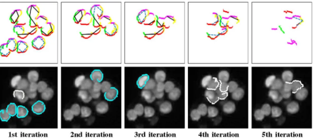
Fig. 8 illustrates graphs constructed in different iterations with indicating the edges of the 4PRIM and 3PRIM patterns that satisfy the standard deviation constraint of the corre-sponding iteration. Here, the edges of the patterns satisfying the constraint are shown as blue dashed lines and the others as black solid lines. This figure also shows selected primitive segments of these patterns.
The nucleus identification essentially groups primitives to form a nucleus. In that sense, it can be regarded as a contour grouping method, which aims to group contour (edge) frag-ments to find object boundaries. However, as opposed to pre-vious contour grouping studies [37], [38], our algorithm defines high-level boundary primitives that are attributed to a type and groups them via searching for structural patterns on a relational graph constructed on these attributed primitives.
C. Region Growing
The previous step identifies the primitives of located nuclei. It is simple to delineate an individual nucleus if its primitives form a closed shape; however, this usually does not occur due to noise and overlayering. One might consider connecting the primitives’ end points by a line but this might result in un-natural boundaries, especially for 3PRIM instances. Moreover, some primitives may have been incorrectly assigned to a nu-cleus in the previous step and must be corrected. For example, in Fig. 9(a), primitives of nuclei for a subimage from Fig. 2(a) are shown. We observe that most nuclei do not have a closed form. Further, the top primitive of the red nucleus (indicated
Fig. 8. Illustration of graphs constructed in different iterations and selected primitive segments in these iterations. In the first row, the graph edges of the 4PRIM and 3PRIM patterns that satisfy the standard deviation constraint of the corresponding iteration are indicated as dashed blue lines and the others as black solid lines. In the second row, selected segments of these 4PRIM and 3PRIM patterns are shown in cyan and white, respectively.
Fig. 9. (a) Primitives identified for different nuclei and (b) nucleus boundaries delineated after the region-growing algorithm.
with an arrow) is incorrectly identified; it contains the top prim-itive of the blue nucleus next to it.
Thus, to better delineate nuclei, we use a region-growing al-gorithm that takes the centroids of each nucleus’ primitives as starting points and grows them considering the primitive loca-tions. We use the primitive locations for two ends: First, a pixel cannot grow in the direction of the outer boundaries of a prim-itive as determined by the primprim-itive type; e.g., a pixel cannot grow to the top outer boundaries of the top primitive. Second, for each nucleus, pixels grown after touching a primitive pixel for this nucleus are excluded from the results. Doing this stops growing without the need for an additional mask, and it also re-sults in better boundaries. In this algorithm, we use the geodesic distance from a pixel to a starting point as the growing crite-rion. Last, to obtain smoother boundaries, we apply majority filtering, using a filter radius of , on the results and fill the holes inside the located nuclei. Example results obtained by this growing step are shown in Fig. 9(b).
IV. EXPERIMENTS
A. Dataset
We conduct our experiments on two datasets of fluorescence microscopy images of human hepatocellular carcinoma (Huh7 and HepG2) cell lines. Because the amount of cells growing in overlayers is much higher in the HepG2 cell line, the cell nu-clei in that dataset are more overlayered than the Huh7 nunu-clei.
This situation makes segmentation more difficult for the HepG2 dataset. To understand the effectiveness of our proposed algo-rithm on the nuclei of less overlayered and more overlayered cells, we test it on both sets separately and observe the segmen-tation performance. These sets contain 2661 nuclei in 37 im-ages, 16 of which belong to the Huh7 and 21 of which belong to the HepG2 cell lines.
Both cell lines were cultured and their images taken in the Molecular Biology and Genetics Department of Bilkent Uni-versity. The cell lines were cultured routinely at 37 under 5% in a standard Dulbecco’s Modified Eagle Medium (DMEM) supplemented with 10% Fetal Calf Serum (FCS). For visualization, nuclear Hoechst 33258 (Sigma) staining was used. The images were taken at 768 1024 resolution, under a Zeiss Axioscope fluorescent microscope with an AxioCam MRm monochrome camera using a 20 objective lens and a
pixel size of . We compare the automated
segmentation results with manually delineated gold standards, where nuclei were annotated by our biologist collaborators.
B. Evaluation
We evaluate the segmentation results visually and quantita-tively. The common metrics for quantitative evaluation are ac-curacy and precision. Acac-curacy measures how close the seg-mentation is to the gold standard, whereas precision measures the reproducibility of multiple segmentations of the same image [39], [40]. In our study, we follow an approach similar to [40] to measure accuracy; however, we do not assess precision be-cause the proposed algorithm is deterministic and always gives the same segmentation for the same image.
We assess accuracy using two methods: nucleus-based and pixel-based. In nucleus-based evaluation, the aim is to assess the accuracy of an algorithm in terms of the number of correctly segmented nuclei. A nucleus is said to be correctly segmented if it one-to-one matches with an annotated nucleus in the gold standard. For that, we first match each computed nucleus to an annotated one and vice versa; a computed nucleus is matched to an annotated nucleus if at least half of ’s area overlaps with . Next, segmented nuclei that form unique pairs with an-notated ones are counted as one-to-one matches, after which nu-cleus-based precision, recall, and F-score are calculated.
Addi-tionally, we consider oversegmentations, undersegmentations,
misses, and false detections. An annotated nucleus is
overseg-mented if two or more computed nuclei match the annotated nu-cleus, and annotated nuclei are undersegmented if two or more match the same computed nucleus. A computed nucleus is a false detection if it does not match any annotated nucleus and an annotated nucleus is a miss if it does not match any computed nucleus.
In pixel-based evaluation, the aim is to assess accuracy in terms of the areas of correctly segmented nuclei. We use the one-to-one matches found in nucleus-based evaluation and consider overlapping pixels of the computed-annotated nucleus pairs of these matches as true positives. Then, we calulate pixel-based precision, recall, and F-score measures.
C. Parameter Selection
The proposed algorithm has four external model parameters: 1) primitive length threshold from the primitive definition and graph construction, 2) percentage threshold from the iterative search algorithm, 3) standard deviation threshold from the cell localization, and 4) radius of the structuring element of the majority filter from the region growing. We se-lect the values of these parameters for the training nuclei. We randomly select five images from each of the Huh7 and HepG2 sets, using 785 nuclei from these 10 images as the training set. We use the nuclei in the rest of the images as the test sets, which include 891 nuclei for the Huh7 and 985 nuclei for HepG2 cell lines.
For parameter selection, we first consider all possible
com-binations of the following values: ,
, , and
. Then, we select the parameter combination that gives the best F-score for the training nuclei. The selected
parameters are pixels, , , and
. We discuss the effects of these parameter values on segmentation performance in the next section. Additionally, an internal parameter is used to define boundary primitives by taking the -outermost pixels of the binary maps of the Sobel responses. Smaller values of are not enough to put the boundaries of the same cell under the same primitive, whereas larger values connect the boundaries of different cells. Thus, we internally set , which gives good primitives in our experiments.
D. Comparisons
We use three comparison algorithms: adaptive h-minima [4], conditional erosion [16], and iterative voting [9]. The algo-rithms from the first two studies implement marker-controlled watersheds; they identify markers based on shape information. Adaptive h-minima [4] obtains a binary segmentation via active contours without edges and calculates an inner distance map that represents the distance from every foreground pixel to the background. Then, it identifies regional minima as the markers, found after applying the h-minima transform to the inverse of the map, and calculates an outer distance map representing the distance from the foreground pixels to their nearest marker. Finally, it grows the markers using the combination of the outer distance map and the gray-scale image as a marking function.
Conditional erosion [16] obtains a binary image by histogram thresholding and iteratively erodes its connected components by a series of two cell-like structuring elements of different sizes. It first uses the larger element until the sizes of the eroded compo-nents fall below a threshold. The component shapes are coarsely preserved due to the size of the structuring element and its round shape. It next uses the smaller element on the remaining com-ponents and stops the iterations just before the component sizes become smaller than a second threshold. Considering the eroded components as the markers, it then applies a watershed algo-rithm on the binary image.
Iterative voting [9] defines and uses a series of oriented kernels for localizing saliency, which corresponds to nucleus centers in a microscopic image. This study localizes the centers from incomplete boundary information by iteratively voting kernels along the radial direction. It continues iterations, in which the shape of the kernel and its orientation are refined, until convergence. It then identifies the centers by thresholding the vote image computed throughout the iterations and outputs a set of centers that can be used as the markers in a watershed algorithm. In our experiments, we use the software provided by the authors of [9], available at http://vision.lbl.gov/Publi-cations/ieee_trans_ip07, to find the nucleus centers and apply a marker-controlled watershed algorithm on the binary image obtained by histogram thresholding. These three comparison algorithms have their own parameters. We also select their values for the training nuclei by following the methodology given in Section IV-C. For details of the algorithms’ parame-ters, the reader is referred to the technical report given in [41].
V. RESULTS
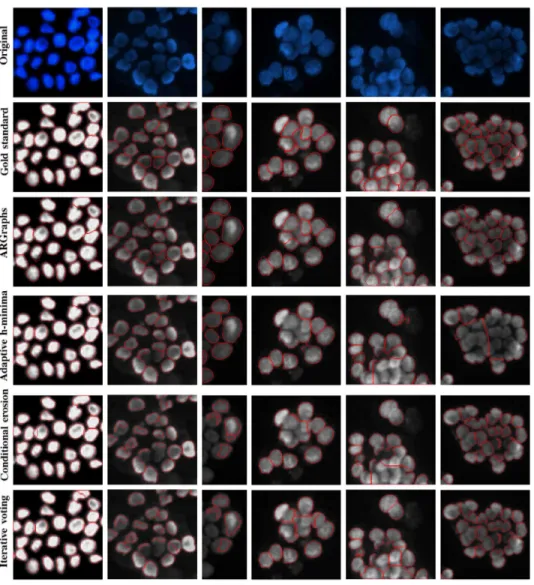
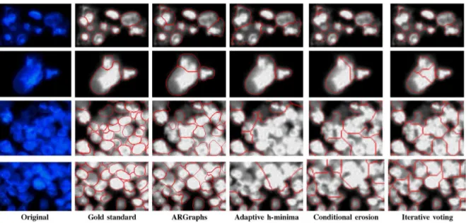
In Fig. 10, we present visual results for example subimages obtained by the algorithms. Note that these subimages are of different sizes, but they have been scaled for better visualiza-tion. Also note that the sizes of the images from which they are cropped are the same and that we run the algorithms on the orig-inal-sized images. Fig. 10 demonstrates that all algorithms can accurately segment the nuclei of monolayer isolated cells (the first column on the left of the figure); however, compared to the others, the proposed algorithm (ARGraphs) better segments the nuclei of touching and more overlayered cells. For these nuclei, the other algorithms commonly lead to more undersegmenta-tions, as also observed in the quantitative results (see Table I).
In Fig. 11, we present the number of one-to-one matches in bar graph form. We provide precision, recall, and F-score mea-sures in Table II. These results show that our ARGraphs al-gorithm improves segmentation performance for both datasets compared to the others. The improvement is more notable for the HepG2 dataset, in which cells are more overlayered. These findings are consistent with the visual results, and we attribute them to the following properties of our algorithm. First, condi-tional erosion and adaptive h-minima heavily rely on an initial map to find their markers. If this map is not accurately deter-mined (which is usually the case) or if there are no background pixels inside a nucleus cluster, these methods are inadequate at separating nuclei in relatively bigger clusters. This failing is ob-served in the results of these algorithms, given in the second and
Fig. 10. Visual results obtained by the algorithms for various subimages. The image sizes have been scaled for better visualization.
TABLE I
COMPARISON OF THEALGORITHMS INTERMS OFCOMPUTED-ANNOTATED
NUCLEUSMATCHES ON THE(a) Huh7AND(b) HepG2 TESTSETS
third columns of Fig. 10. The problem is more obvious in the re-sults of conditional erosion, which uses global thresholding to obtain its map. Our algorithm uses an initial map to find local thresholds but nowhere else, which makes it more robust to in-accuracies of this map.
Second and more importantly, our algorithm uses the fact that a nucleus should have four boundaries, each of which locates
Fig. 11. Number of one-to-one matches for the Huh7 and HepG2 test sets.
one of its four sides, in its segmentation. This helps our algo-rithm identify nuclei even when their boundaries are only par-tially present (using the 4PRIM pattern) or even when one of the boundaries missing (using the 3PRIM pattern). In this way, we can (to a degree) compensate for the negative effects of over-layered nuclei. This property is evident in the last three columns of Fig. 10. It is worth noting that iterative voting also does not require an initial map to find nucleus centers; however, in using
TABLE II
COMPARISON OF THEALGORITHMS INTERMS OFNUCLEUS-BASED ANDPIXEL-BASEDPRECISION, RECALL,ANDF-SCOREMEASURES
ON THE(a) Huh7AND(b) HepG2 TESTSETS
shape information to define its kernels, it may give incorrect re-sults when nuclei appear in irregular shapes due to overlayering. When we analyze the nucleus centers found by iterative voting, we observe that this algorithm usually fails to find nuclei that are partially obscured by others.
Another class of methods uses filters (such as sliding band filters [32] and Laplacian of Gaussians [33]) to detect nuclei by considering the nucleus’ blob-like convex shape. They identify places with high filter responses as initial nucleus locations, and further process them to find nucleus borders. These methods can give good initial locations especially for the nuclei of monolayer isolated cells; however, when cell nuclei appear in irregular and nonconvex shapes due to overlayering, they can lead to incorrect initial nucleus locations.
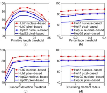
A. Parameter Analysis
We investigate the effects of each parameter on the perfor-mance of the proposed algorithm. To this end, we fix three of the four parameters and observe the changes in nucleus-based and pixel-based F-score measures with respect to different values of the other parameter. In Fig. 12, we present the analysis results separately for the Huh7 and HepG2 test sets.
The first parameter is the primitive length threshold , which is used in defining the primitives and constructing the graphs. In the former, primitive components whose width/height is smaller than are eliminated because they are more likely to be noise than nucleus boundaries. Likewise, in the latter, primitives smaller than are not considered part of a structural pattern. Larger values of this parameter eliminate more primitives, especially the ones belonging to small nuclei, and also increase misses and undersegmentations. On the other hand, smaller thresholds increase the number of false primitives, which results in more false detections and oversegmentations. As observed in Fig. 12(a), these both lower the F-score measures.
The second parameter is the percentage threshold used by the iterative search algorithm. This algorithm searches for structural patterns on the graph , which is constructed on primitives identified by thresholding the Sobel responses. Ini-tial thresholds are computed using the Otsu method and relaxed in later iterations to find more primitives. However, there must
Fig. 12. For the Huh7 and HepG2 test sets, cell-based and pixel-based F-score measures as a function of the (a) primitive length threshold , (b) percentage threshold , (c) standard deviation threshold , and (d) radius of the structuring element.
be a limit to this relaxation because too-small thresholds (as a result of several iterations) falsely identify noise as primitives. Thus, we use a threshold to stop iterations so that segmentation is not affected by these falsely identified primitives. Smaller values yield more false detections, which lower F-scores, as observed in Fig. 12(b).
The next parameter is the standard deviation threshold used in nucleus localization. In the iterative search algorithm, structural patterns are identified as nuclei if they satisfy the shape constraint, which is based on their standard deviation. When smaller thresholds are used, the nucleus candidates need to be rounder to be detected. For this reason, the algorithm can find only a few structural patterns, which lowers the number of one-to-one matches thus decreasing F-scores [see Fig. 12(c)]. The last parameter is radius of the structuring element of the majority filter. This parameter is used in region growing, which applies majority filtering on segmented nuclei to smooth their boundaries. The results given in Fig. 12(d) show that this pa-rameter affects performance the least.
B. Discussion
The experiments show that our ARGraphs algorithm leads to promising results for the nuclei of isolated and overlayered cells. They also show that the algorithm is robust to a certain amount of pixel-level noise, which typically arises from nonideal ex-perimental conditions such as weak staining and poor back-ground illumination. These findings are attributed to the fol-lowing: The ARGraphs algorithm models high-level relational dependencies between the attributed boundary primitives in-stead of directly using an initial map or gradients defined at the pixel-level. Moreover, it follows an iterative approach to define the primitives, doing so on relatively high Sobel responses in its early iterations and on lower ones in later iterations. Thus, boundaries that appear broken in initial iterations may later be-come complete.
Fig. 13. Top two rows: results for subimages containing inner intensity variation and texture. Bottom two rows: results for subimages containing very dense nucleus clusters. The sizes of the subimages have been scaled for better visualization.
This iterative nature of the algorithm also helps handle inner-nuclear texture to some degree. Because of this texture, it is pos-sible to find pixels with high responses inside a nucleus. How-ever, the magnitudes of these responses are generally lower than those of the pixels found on nucleus contours. For this reason, it is more likely to define primitives on contour pixels and thus to form a nucleus on these primitives in earlier iterations. Be-cause we exclude primitive segments of the selected nucleus from later iterations, primitives defined on textured regions do not typically introduce new nucleus fragments. A primitive can be defined on pixels only if these pixels form a connected com-ponent with a length greater than . Textured regions can thus lead to primitives when the texture granularity is large enough, but defining a primitive does not automatically define a nucleus; to do that, the primitive must be part of a 3PRIM or 4PRIM pattern. This criterion further decreases the likelihood of tex-tured regions leading to unwanted nucleus fragments. We ana-lyze the results of the algorithms on subimages containing some inner-nuclear intensity variation and texture, and as seen in the first two rows of Fig. 13, our algorithm performs better than the others.
When images contain too-dense nucleus clusters with some texture and noise, the accuracy of the proposed algorithm de-creases. Examples of such subimages are given in the last two rows of Fig. 13. However, as also evident in this figure, the problem becomes more difficult for all algorithms, and even for humans. As a future work, one could explore incorporating tex-ture featex-tures into primitive definition to locate better boundary primitives, which may increase accuracy.
VI. CONCLUSION
This paper presents a new model-based algorithm for seg-menting nuclei in fluorescence microscopy images. This algo-rithm models how a human locates a nucleus by identifying the boundaries of its four sides. To this end, the model defines high-level primitives to represent the boundaries and transforms
nucleus identification into a problem of identifying predefined structural patterns in a graph constructed on these primitives. In region growing, it then uses the primitives to delineate the nu-cleus borders. The proposed algorithm is tested on 2661 nuclei taken from two different cell lines and the experiments reveal that it leads to better results for isolated monolayer and more overlayered cells than its counterparts.
This work uses an iterative algorithm to search for struc-tural patterns in the attributed relational graph defined on the boundary primitives. This search algorithm uses a greedy ap-proach, which selects the locally optimal instance at each stage. This instance is the one, for which the standard deviation of ra-dial distances from the outer boundaries of its primitives is the smallest. One may consider this algorithm as an approximation of a much harder combinatorial optimization problem. Given a set of primitives defined in different iterations, locate structural patterns to minimize the sum of the standard deviation of all se-lected instances. This problem requires an exhaustive search to find the globally optimal solution. The greedy approach, how-ever, gives a feasible solution although it does not guarantee finding the global optimum. Different search algorithms could also be implemented to find a better solution to this problem. For example, one could define a probability function for the stan-dard deviation metric of instances. At each stage, an instance could probabilistically be selected using this function instead of selecting the one with the smallest metric. Repeating this algo-rithm many times, multiple segmentation results would be ob-tained and combined in an ensemble to find the final segmen-tation. Exploring different search algorithms is another future research direction for this work.
The proposed model locates the primitives using Sobel oper-ators and attributes them to a type based on the orientation of this operator. We use the Sobel operator because it is relatively simple and effective for our experiments. Nevertheless, another gradient operator could be used to locate the primitives. One could extract features from the primitives and attribute them to
a type, using the extracted features in a classifier. However, in that case, the classifier would need to be trained, which would require determining a set of labels for training primitives, which may not be straightforward. Using different methods to locate and attribute the primitives could be another future research di-rection.
REFERENCES
[1] X. Chen, X. Zhou, and S. T. Wong, “Automated segmentation, classi-fication, and tracking of cancer cell nuclei in time-lapse microscopy,”
IEEE Trans. Biomed. Eng., vol. 53, no. 4, pp. 762–766, Apr. 2006.
[2] A. A. Dima, J. T. Elliott, J. J. Filliben, M. Halter, A. Peskin, J. Bernal, M. Kociolek, M. C. Brady, H. C. Tang, and A. L. Plant, “Comparison of segmentation algorithms for fluorescence microscopy images of cells,”
Cytom. Part A, vol. 79A, pp. 545–559, 2011.
[3] C. Wahlby, I.-M. Sintor, F. Erlandsson, G. Borgefors, and E. Bengtsson, “Combining intensity, edge and shape information for 2D and 3D seg-mentation of cell nuclei in tissue sections,” J. Microsc., vol. 315, pp. 67–76, 2004.
[4] J. Cheng and J. C. Rajapakse, “Segmentation of clustered nuclei with shape markers and marking function,” IEEE Trans. Biomed. Eng., vol. 56, no. 3, pp. 741–748, Mar. 2009.
[5] M. Wang, X. Zhou, F. Li, J. Huckins, R. W. King, and S. T. C. Wong, “Novel cell segmentation and online SVM for cell cycle phase identi-fication in automated microscopy,” Bioinformatics, vol. 24, no. 1, pp. 94–101, 2008.
[6] K. Nandy, P. R. Gudla, R. Amundsen, K. J. Meaburn, T. Misteli, and S. J. Lockett, “Automatic segmentation and supervised learning-based selection of nuclei in cancer tissue images,” Cytom. Part A, vol. 81A, pp. 743–754, 2012.
[7] N. Kharma, H. Moghnieh, J. Yao, Y. P. Guo, A. Abu-Baker, J. La-ganiere, G. Rouleau, and M. Cheriet, “Automatic segmentation of cells from microscopic images using ellipse detection,” IET Image Process., vol. 1, no. 1, pp. 39–47, 2007.
[8] S. Kumar, S. H. Ong, S. Ranganath, T. C. Ong, and F. T. Chew, “A rule-based approach for robust clump splitting,” Pattern Recognit., vol. 39, pp. 1088–1098, 2006.
[9] B. Parvin, Q. Yang, J. Han, H. Chang, B. Rydberg, and M. H. Bar-cellos-Hoff, “Iterative voting for inference of structural saliency and characterization of subcelluar events,” IEEE Trans. Med. Imag., vol. 16, no. 3, pp. 615–623, Mar. 2007.
[10] D. Fenistein, B. Lenseigne, T. Christophe, P. Brodin, and A. Gen-ovesio, “A fast, fully automated cell segmentation algorithm for high-throughput and high-content screening,” Cytometry A, vol. 73, pp. 958–964, 2008.
[11] Z. Yin, R. Bise, M. Chen, and T. Kanade, “Cell segmentation in microscopy imagery using a bag of local Bayesian classifiers,” in
Proc. IEEE Int. Symp. Biomed. Imag.: From Nano to Macro, 2010,
pp. 125–128.
[12] F. Bunyak, K. Palaniappan, S. K. Nath, T. I. Baskin, and G. Dong, “Quantitative cell motility for in vitro wound healing using level set-based active contour tracking,” in Proc. IEEE Int. Symp. Biomed.
Imag.: From Nano to Macro, 2006, pp. 1040–1043.
[13] G. Xiong, X. Zhou, and L. Ji, “Automated segmentation of drosophila RNAi fluorescence cellular images using deformable models,” IEEE
Trans. Circuits Syst. I, vol. 53, no. 11, pp. 2415–2424, 2006.
[14] S. K. Nath, K. Palaniappan, and F. Bunyak, “Cell segmentation using coupled level sets and graph-vertex coloring,” in Proc. Med. Image
Comput. Assist. Interv., 2006, vol. 9, pp. 101–108.
[15] J. Lindblad, C. Wahlby, L. Ji, E. Bengtsson, and A. Zaltsman, “Image analysis for automatic segmentation of cytoplasms and classification of Rac1 activation,” Cytometry A, vol. 57A, no. 22–33, 2004. [16] X. Yang, H. Li, and X. Zhou, “Nuclei segmentation using marker
con-trolled watershed, tracking using mean-shift, and Kalman filter in time-lapse microscopy,” IEEE Trans. Circuits Syst. I, vol. 53, no. 11, pp. 2405–2414, 2006.
[17] H. Zhou and K. Z. Mao, “Adaptive successive erosion-based cell image segmentation for p53 immunohistochemistry in bladder inverted papil-loma,” in Proc IEEE Eng. Med. Biol. Soc., 2005, pp. 6484–6487. [18] C. Jung, C. Kim, S. W. Chae, and S. Oh, “Unsupervised
segmenta-tion of overlapped nuclei using Bayesian classificasegmenta-tion,” IEEE Trans.
Biomed. Eng., vol. 57, no. 12, pp. 2825–2832, Dec. 2010.
[19] P. S. U. Adiga and B. B. Chaudhuri, “An efficient method based on watershed and rule-based merging for segmentation of 3-D histopatho-logical images,” Pattern Recognit., vol. 34, pp. 1449–1458, 2001. [20] P. R. Gudla, K. Nandy, J. Collins, K. J. Meaburn, T. Mitseli, and S. J.
Lockett, “A high-throughput system for segmenting nuclei using multi-scale techniques,” Cytometry A, vol. 73A, pp. 451–466, 2008. [21] G. Lin, M. K. Chawla, K. Olson, J. F. Guzowski, C. A. Barnes, and
B. Roysam, “Hierarchical, model-based merging of multiple fragments for improved three-dimensional segmentation of nuclei,” Cytometry A, vol. 63A, pp. 20–33, 2005.
[22] X. Zhou, F. Li, J. Yan, and S. T. C. Wong, “A novel cell segmenta-tion method and cell phase identificasegmenta-tion using Markov model,” IEEE
Trans. Inf. Technol. Biomed., vol. 13, no. 2, pp. 152–157, Mar. 2009.
[23] G. Lin, U. Adiga, K. Olson, J. F. Guzowski, C. A. Barnes, and B. Roysam, “A hybrid 3D watershed algorithm incorporating gradient cues and object models for automatic segmentation of nuclei in con-focal image stacks,” Cytometry A, vol. 56A, pp. 23–36, 2003. [24] O. Schmitt and S. Reetz, “On the decomposition of cell clusters,” J.
Math. Imag. Vis., vol. 22, no. 1, pp. 85–103, 2009.
[25] Q. Wen, H. Chang, and B. Parvin, “A Delaunay triangulation approach for segmenting clumps of nuclei,” in Proc. IEEE Int. Symp. Biomed.
Imag.: From Nano to Macro, 2009, pp. 9–12.
[26] S. Kothari, Q. Chaudry, and M. D. Wang, “Automated cell counting and cluster segmentation using concavity detection and ellipse fitting technique,” in Proc. IEEE Int. Symp. Biomed. Imag.: From Nano to
Macro, 2009, pp. 795–798.
[27] M. Farhan, O. Yli-Harja, and A. Niemisto, “A novel method for splitting clumps of convex objects incorporating image intensity and using rectangular window-based concavity point-pair search,” Pattern
Recognit., vol. 46, no. 3, pp. 741–751, 2013.
[28] O. Schmitt and M. Hasse, “Radial symmetries based decomposition of cell clusters in binary and gray level images,” Pattern Recognit., vol. 41, no. 6, pp. 1905–1923, 2008.
[29] X. Qi, F. Xing, D. J. Foran, and L. Yang, “Robust segmentation of over-lapping cells in histopathology specimens using parallel seed detection and repulsive level set,” IEEE Trans. Biomed. Eng., vol. 59, no. 3, pp. 754–765, Mar. 2012.
[30] H. Kong, M. Gurcan, and K. Belkacem-Boussaid, “Partitioning histopathological images: An integrated framework for supervised color-texture segmentation and cell splitting,” IEEE Trans. Med.
Imag., vol. 30, no. 9, pp. 1661–1677, Sep. 2011.
[31] T. Jiang, F. Yang, and Y. Fan, “A parallel genetic algorithm for cell image segmentation,” Electron. Notes Theo. Comp. Sci., vol. 46, pp. 1–11, 2001.
[32] P. Quelhas, M. Marcuzzo, A. M. Mendonca, and A. Campilho, “Cell nuclei and cytoplasm joint segmentation using sliding band filter,”
IEEE Trans. Med. Imag., vol. 29, no. 8, pp. 1463–1473, Aug. 2010.
[33] Y. Al-Kofahi, W. Lassoued, W. Lee, and B. Roysam, “Improved auto-matic detection and segmentation of cell nuclei in histopathology im-ages,” IEEE Trans. Biomed. Eng., vol. 57, no. 4, pp. 841–852, Apr. 2010.
[34] V. S. Lempitsky and A. Zisserman, “Learning to count objects in im-ages,” Proc. Adv. Neural Inf. Process. Syst., pp. 1324–1332, 2010. [35] O. Sertel, G. Lozanski, A. Shana’ah, and M. N. Gurcan,
“Computer-aided detection of centroblasts for follicular lymphoma grading using adaptive likelihood-based cell segmentation,” IEEE Trans. Biomed.
Eng., vol. 57, no. 10, pp. 2613–2616, Oct. 2010.
[36] T. F. Chan and L. A. Vese, “Active contours without edges,” IEEE
Trans. Image Process., vol. 10, no. 2, pp. 266–277, Feb. 2001.
[37] Q. Zhu, G. Song, and J. Shi, “Untangling cycles for contour grouping,” in Proc. IEEE Int. Conf. Comp. Vis., 2007, pp. 1–8.
[38] J. H. Elder, A. Krupnik, and L. A. Johnston, “Contour grouping with prior models,” IEEE Trans. Pattern Anal. Mach. Intell., vol. 25, no. 6, pp. 661–674, Jun. 2003.
[39] S. K. Warfield, K. H. Zou, and W. M. Wells, “Simultaneous truth and performance level estimation (STAPLE): An algorithm for the valida-tion of image segmentavalida-tion,” IEEE Trans. Med. Imag., vol. 23, no. 7, pp. 903–921, Jul. 2004.
[40] J. K. Udupa, V. R. LeBlanc, Y. Zhuge, C. Imielinska, H. Schmidt, L. M. Currie, B. E. Hirsch, and J. Woodburn, “A framework for evaluating image segmentation algorithms,” Comput. Med. Imag. Grap., vol. 30, pp. 75–87, 2006.
[41] S. Arslan, T. Ersahin, R. Cetin-Atalay, and C. Gunduz-Demir, Attributed relational graphs for cell nucleus segmentation in fluores-cence microscopy images: Supplementary Material Comput. Eng., Bilkent Univ., Tech. Rep. BU-CE-1301, 2013 [Online]. Available: http://www.cs.bilkent.edu.tr/tech-reports/2013/BU-CE-1301.pdf