Comparisons of six different estimation methods for log-Kumaraswamy distribution

COMPARISONS OF SIX DIFFERENT ESTIMATION METHODS

FOR LOG-KUMARASWAMY DISTRIBUTION

by

Caner TANIS * _{and Bugra SARACOGLU} Faculty of Science, Selcuk University, Konya, Turkey

Original scientific paper https://doi.org/10.2298/TSCI190411344T

In this paper, it is considered the problem of estimation of unknown parameters of log-Kumaraswamy distribution via Monte-Carlo simulations. Firstly, it is de-scribed six different estimation methods such as maximum likelihood, approximate bayesian, least-squares, weighted least-squares, percentile, and Cramer-von-Mis-es. Then, it is performed a Monte-Carlo simulation study to evaluate the perfor-mances of these methods according to the biases and mean-squared errors of the estimators. Furthermore, two real data applications based on carbon fibers and the gauge lengths are presented to compare the fits of log-Kumaraswamy and other fitted statistical distributions.

Key words: log-Kumaraswamy distribution, maximum likelihood estimation,

Cramer-von-Mises estimation method, least-squares estimation, percentile estimation, Monte-Carlo simulation

Introduction

Log-Kumaraswamy (LKw) distribution is a special case of log-exponentiated Ku-maraswamy distribution proposed by Lemonte et al. [1]. They have generated LKw distribution by using a log-transform in cumulative distribution function (cdf) of Kumaraswamy (Kw) dis-tribution suggested by Kumaraswamy [2]. Let Y be a random variable having Kw disdis-tribution with parameters a and b. The LKw distribution is obtained by X = –log(1 – Y) transformation. The cdf, the probability density function (pdf), and hazard rate function (hf):

(

)

(

)

1

(

)

1 ; , x 1 e x a 1 1 e x a b f x a b ₌abe− ₋ − −  _{− −} −  −     (1)

(

, ,

)

1 1 1 e

(

x

)

a b F x a b _{= − − −} −      (2)

(

)

(

)

(

)

1 1 e ; , 1 1 e a x x a x abe h x a b − − − − − =  _{− −}      (3) where a > 0, b > 0, and x > 0. The LKw(a, b) distribution can be useful in order to model real data in areas such as hydrology, engineering, science, medicine, agriculture, etc.

Some studies on LKw distribution can be listed as follows. Mohammed [3] studied inference on the log-exponentiated Kw distribution. Chacko and Mohan [4] investigated the

problem of the estimation of parameters for Kw-exponential distribution under progressive type-II censoring. Akinsete et al. [5] proposed Kw-geometric distribution. Moreover, Jose and Varghese [6] introduced Wrapped LKw distribution. Korkmaz and Genc [7] suggested two-sid-ed generaliztwo-sid-ed exponential distribution. Korkmaz and Genc [8] introductwo-sid-ed a new lifetime dis-tribution based on a transformation of two sided power variate. The problem of parameter estimation for many distributions is very popular. In recent years, there are many extensive studies on parameter estimation for various distributions in literature. Ramos and Louzada [9] have introduced a new distribution called as the generalized weighted lindley distribution and studied different methods of estimation for this distribution. Dey et al. [10] have compared the methods of estimation for Nadarajah and Haghighi distribution. Dey et al. [11] have studied different estimation methods for Kw distribution. Also, in [12] they estimated the parameters of Gompertz distribution using different estimation methods. Ramos et al. [13] have consid-ered the problem of estimation of parameters for Frechet distribution. Balakrishnan and Kundu [14] presented an extensive study including new estimation methods and extensions for Birn-baum-Saunders distribution.

The aim of this article is to compare the performances of methods of estimation for LKw(a, b) distribution via Monte-Carlo simulations and real data applications. For this reason, six different estimation methods such as the maximum likelihood, approximate bayesian, least-squares, weighted least-least-squares, percentile and Cramer-von-Mises are considered.

Estimation methods

Maximum likelihood estimates

Let X1, X2,...,Xn be a random sample taken from LKw(a, b) distribution. The log-like-lihood function:

(

)

(

)

(

)

(

)

(

)

(

)

1 1

, | log log 1 log 1

1 log 1 1 e n n i i a b n a b x a e = = = + − + − − +   + − _ − − _  

∑

∑

∑

(4)

The maximum likelihood estimators (MLE) of unknown parameters are derived by maximizing the log-likelihood function in eq. (4). The likelihood equations are also obtained from the partial derivatives of log-likelihood function with respect to a and b parameters. These derivates are:

(

)

₍

₎

₍

₎

(

) (

)

(

)

1 1 1 e log 1 e , | log 1 e 1 1 1 e i i i i a x x n n x a x i i a b n _b a a − − − − = = − − ∂ = + − − − ∂

∑

∑

_{− −} x  (5)

(

)

₍

₎

1 , | log 1 1 e i n _a x i a b n b b − = ∂ _{ } = + _ − − _   ∂

∑

x  ₍₆₎ The MLE, a^

MLE and b^MLE, can be obtained by solving of likelihood equations, in eqs. (5) and (6). These non-linear equations can be solved by some numerical methods.

Approximate bayesian estimates

Let X1, X2,...,Xn be a random sample with size n taken from LKw(a, b) distribution. In this study, the independent gamma priors for a and b parameters are used:

( )

1 1 1 1 1 e , , , 0 d ae a a − − a e d π ∝ > ₍₇₎

( )

2 1 2 2 2 e , , , 0 d be b b − − b e d π ∝ > ₍₈₎

The joint priors and posterior distributions of a and b parameters, are given by, re-spectively:

( )

a b,

( ) ( )

a b a bd1−1 d2−1e−(ae be1+ 2) π = π π ∝ ₍₉₎

(

)

(

_{( )}

) ( )

( )

( )

0 0 | , , ( ; , ) , , | ( ; , ) , d d x f a b a b w a b a b a b f x ∞ ∞_{w a b a b a b} π π π = = π

∫∫

x x x x (10) where

(

) ( )

1

(

)

(

)

1 1 1 ; , e 1 e 1 1 e n i i i i b n x _{a a} n x x i w a b ab = − − ₋ − − = ∑ _{ } = − _ − − _  

∏

x

Thus, Bayes estimator (BE) under squared loss function for any function of a and b, say u(a, b):

( )

( )

(

)

( ) ( ) ( ) ( ) , | , 0 0 , | , 0 0 , | e d d , , | e d d a b a b B a b a b u a b a b u a b E u a b a b ρ ρ             ∞ ∞ + ∧ ∞ ∞ +     = =

∫∫

∫∫

x x x x   (11)

where 𝓁(a, b | x) is log-likelihood function, ρ(a, b) – the logarithm of joint prior distribution. It is difficult to get the integral presented in eq. (11) in closed form. Some approximate methods to get the integrals are used. One of these methods is Tierney Kadane’s approximation method.

Bayes estimates with Tierney and Kadane’s method

Tierney and Kadane’s approximation introduced by Tierney and Kadane [15] to com-pute integral ratios. In Bayes analysis has been studied by many authors such as Danish and Aslam [16], Gencer and Saracoglu [17], Kumar [18], Kinaci et al. [19], Tanis and Saracoglu [20], Jung and Chung [21]. Tierney and Kadane approximation can be summarized:

( )

, 1

{

( ) (

, , |

)

}

I a b a b a b n ρ = + x (12)

( )

( ) ( )

* _, 1_{log , ,} I a b u a b I a b n = + ₍₁₃₎

where ρ(a, b) is defined:

( ) (

a b, d1 1 log

) ( ) (

a d2 1 log

) ( ) (

b ae be1 2

)

ρ = − + − − + ₍₁₄₎

The BE with Tierney and Kadane approximation of u(a, b) under squared error loss function for LKw(a, b):

( )

( )

( ) ( )

{

(

) ( )

}

* * * , 1 2 * * 0 0 , 0 0 d d det _{ˆ ˆ} ˆ , , | exp ˆ , ˆ , det d d nI a b b I I I I nI a b e a b u a b E u a b n I a b I a b e a b ∞ ∞ ∞ ∞ _{ Σ }      = _ _= = _{  } − _ Σ     

∫∫

∫∫

x (15) where (a^

I*, b^I*) and (a^ I, b^I) maximize I*(a^ I*, b^I*)and I(a^ I, b^I), respectively. The ∑* and ∑ are minus the inverse Hessians of I*_(a^

Least square and weighted least squares estimates

Let X1:n ≤ X2:n ≤... ≤ Xn:n be order statistics of a random sample with n sizes having LKw (a, b) distribution. Then, the expected value of the empirical cumulative distribution function (ecdf):

(

)

(

)

(

)

(

) (

)

: : 2 1 , , 1,2,..., 1 1 2 i n i n i n i i E F X Var F X i n n _{n n} − + = = =       ₊   _{+ +} (16)

The least square estimates of a and b, a^

LSE and b^LSE can be obtained by minimizing following eq. (17):

( )

(

:

)

2 1 , 1 1 1 e 1 i n n _a b x i i Z a b n − =  _{ }  =  − − −_{ } −  +  

∑

(17) In this case, a^

LSE and b^ LSE can be obtained via the simultaneously solution of the fol-lowing system of equations:

( )

₍

₎

₍

:

₎

: 1 , , , 1 1 1 e 0 1 i n n _a b x i n i Z a b _{k x a b} i a n − = ∂ ₌  _{− − −  −} ₌  _{ }  ∂

∑

_ + _ (18)

( )

₍

₎

₍

:

₎

: 1 , g , , 1 1 1 e 0 1 i n n _a b x i n i Z a b _{x a b} i b n − = ∂ ₌  _{− − −  −} ₌  _{ }  ∂

∑

_ + _ (19) where

(

)

(

:

)

(

:

) (

:

)

1 : , , 1 1 e i n 1 e i n log 1 e i n b a a x x x i n k x a b ₌b _{− −} −  − ₋ − ₋ −    

(

)

(

:

)

(

:

)

: g , , log 1 1 e i n 1 1 e i n b a a x x i n x a b _{= −}  _{− −} −   _{− −} −         

Equations (18) and (19) can be simultaneously solved using some iterative methods. The weighted least squared estimators (WLSE) shown with a^

WLSE and b^WLSE can be obtained by minimizing following equation with respect to a and b parameters:

( )

(

:

)

2 1 , 1 1 1 e 1 i n n _a b x i i i a b n ϖ τ − =  _{ }  =  − − −_{ } −  +  

∑

(20) where

(

)

(

(

) (

)

)

2 : 1 2 1 1 i i n n n i n i Var F X τ = = + + − +     Percentile estimates

In this subsection, the percentile estimates (PE) of a and b for LKw(a, b) distribution,

a^

PE and b^PE are obtained. This estimation method was firstly suggested by Kao [22, 23]. There are many studies based on percentile estimation of unknown parameters for various statistical distributions. Some of these studies are Gupta and Kundu [24], Alkasabeh and Raqab [25], Erisoglu and Erisoglu [26]. The quantile function of LKw (a, b):

( )

_{, log 1 1 1}

{

(

)

1/b 1/a

}

i

Q a b _{= − − − −} p 

  (21)

Let xi:n is be value of ith order statistics. The a^PE and b^PE can be obtained by minimizing the following equation with respect to a and b parameters:

( )

2 1/ 1/ : 1 , log 1 1 1 1 a b n i n i i a b x n κ =   _{ }   _   _ =  + _ − − − _{ +} _  _    _   _  

∑

(22)

Cramer-von Mises estimates

The Cramer-von Mises estimator is one of the goodness of-fit estimators. This method is based on the difference between the estimate of the cdf and ecdf. The bias of these estimators is smaller than the bias of other minimum distance estimators studied by Luceno [27], Ramos and Louzada [9] and Macdonald [28]. The Cramer-von Mises estimators (CVME), a^

CVME and

b^CVME, can be derived by minimizing following equation:

( )

(

:

)

2 1 1 2 1 , 1 1 1 e 12 i n 1 n _a b x i i C a b n n − = −  _{ }  = +  − − −_{ } −  +  

∑

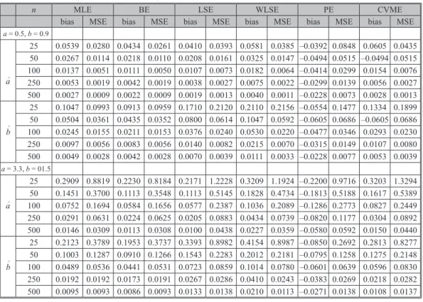
(23) Simulation study

In this section, it is performed a extensive Monte-Carlo simulation study in order to compare MLE, BE, LSE, WLSE, PE, and CVME for LKw(a, b) distribution. The biases and mean square errors (MSE) of these estimators are simulated based on 10000 repetitions by con-sidering different samples of sizes such as 25, 50, 100, 250, and 500 and different initial values as (a = 0.5, b = 0.9), (a = 3.3, b = 1.5), (a = 2.3, b = 1.2) and (a = 4, b = 2) for LKw(a, b) distri-bution. In the bayesian analysis, we consider (d1 = 0.01, e1 = 0.01) and (d2 = 0.01, e2 = 0.01) as the values of prior parameters. The results of simulation study are given in tabs. 1 and 2.

Table 1. The biases and MSE of a^ _{and b}^ _{by using different estimation}

methods for a = 0.5, b = 0.9 and a = 3.3, b = 1.5

n MLE BE LSE WLSE PE CVME

bias MSE bias MSE bias MSE bias MSE bias MSE bias MSE

a = 0.5, b = 0.9 a^ 25 0.0539 0.0280 0.0434 0.0261 0.0410 0.0393 0.0581 0.0385 –0.0392 0.0848 0.0605 0.0435 50 0.0267 0.0114 0.0218 0.0110 0.0208 0.0161 0.0325 0.0147 –0.0494 0.0515 –0.0494 0.0515 100 0.0137 0.0051 0.0111 0.0050 0.0107 0.0073 0.0182 0.0064 –0.0414 0.0299 0.0154 0.0076 250 0.0053 0.0019 0.0042 0.0019 0.0038 0.0027 0.0075 0.0022 –0.0299 0.0139 0.0056 0.0027 500 0.0027 0.0009 0.0022 0.0009 0.0019 0.0013 0.0040 0.0011 –0.0228 0.0073 0.0028 0.0013 b ^ 25 0.1047 0.0993 0.0913 0.0959 0.1710 0.2120 0.2110 0.2156 –0.0554 0.1477 0.1334 0.1899 50 0.0504 0.0361 0.0435 0.0352 0.0800 0.0614 0.1047 0.0592 –0.0605 0.0686 –0.0605 0.0686 100 0.0245 0.0155 0.0211 0.0153 0.0376 0.0240 0.0530 0.0220 –0.0477 0.0346 0.0293 0.0230 250 0.0097 0.0056 0.0083 0.0056 0.0140 0.0082 0.0215 0.0070 –0.0315 0.0149 0.0107 0.0080 500 0.0049 0.0028 0.0042 0.0028 0.0070 0.0039 0.0111 0.0033 –0.0228 0.0077 0.0053 0.0039 a = 3.3, b = 01.5 a^ 25 0.2909 0.8819 0.2230 0.8184 0.2171 1.2228 0.3209 1.1924 –0.2200 0.9716 0.3203 1.3294 50 0.1451 0.3700 0.1113 0.3548 0.1113 0.5145 0.1828 0.4734 –0.1813 0.5188 0.1617 0.5389 100 0.0752 0.1694 0.0584 0.1656 0.0577 0.2387 0.1036 0.2089 –0.1286 0.2773 0.0827 0.2449 250 0.0291 0.0631 0.0224 0.0625 0.0205 0.0883 0.0434 0.0739 –0.0820 0.1177 0.0304 0.0892 500 0.0146 0.0309 0.0113 0.0308 0.0100 0.0438 0.0227 0.0359 –0.0580 0.0592 0.0150 0.0440 b ^ 25 0.2123 0.3789 0.1953 0.3737 0.3393 0.8982 0.4154 0.8987 –0.0850 0.2692 0.2813 0.8277 50 0.1003 0.1287 0.0910 0.1266 0.1543 0.2283 0.2012 0.2181 –0.0795 0.1258 0.1275 0.2148 100 0.0489 0.0536 0.0441 0.0531 0.0723 0.0859 0.1014 0.0780 –0.0601 0.0639 0.0596 0.0830 250 0.0192 0.0192 0.0173 0.0191 0.0267 0.0286 0.0410 0.0243 –0.0383 0.0269 0.0218 0.0282 500 0.0095 0.0093 0.0086 0.0093 0.0133 0.0138 0.0210 0.0113 –0.0271 0.0138 0.0108 0.0137

Table 2. The biases and MSE of a^ _{and b}^ _{by using different estimation methods} for a = 2.3, b = 1.2 and a = 4, b = 2

n MLE BE LSE WLSE PE CVME

bias MSE bias MSE bias MSE bias MSE bias MSE bias MSE a = 2.3 b = 1.2 a^ 25 0.2197 0.4875 0.1716 0.4532 0.1649 0.6781 0.2398 0.6624 –0.1639 0.6212 0.2435 0.7421 50 0.1093 0.2025 0.0854 0.1943 0.0843 0.2825 0.1357 0.2598 –0.1428 0.3400 0.1225 0.2971 100 0.0564 0.0921 0.0446 0.0900 0.0436 0.1303 0.0766 0.1140 –0.1042 0.1848 0.0625 0.1340 250 0.0218 0.0342 0.0171 0.0339 0.0155 0.0480 0.0319 0.0401 –0.0682 0.0799 0.0230 0.0486 500 0.0110 0.0168 0.0087 0.0168 0.0076 0.0238 0.0168 0.0195 –0.0488 0.0409 0.0114 0.0239 b ^ 25 0.1556 0.2097 0.1397 0.2046 0.2508 0.4733 0.3083 0.4773 –0.0687 0.1693 0.2026 0.4305 50 0.0741 0.0735 0.0657 0.0720 0.1155 0.1280 0.1510 0.1228 –0.0648 0.0804 0.0933 0.1198 100 0.0361 0.0310 0.0319 0.0306 0.0543 0.0490 0.0763 0.0446 –0.0492 0.0412 0.0437 0.0472 250 0.0142 0.0112 0.0125 0.0111 0.0201 0.0165 0.0309 0.0141 –0.0315 0.0175 0.0160 0.0162 500 0.0071 0.0055 0.0063 0.0055 0.0100 0.0079 0.0159 0.0066 –0.0222 0.0091 0.0079 0.0079 a = 4 b = 2 a^ 25 0.3186 1.1454 0.2391 1.0634 0.2287 1.5822 0.3506 1.5239 –0.2415 1.1483 0.3426 1.7043 50 0.1543 0.4656 0.1146 0.4467 0.1145 0.6602 0.1993 0.6019 –0.1981 0.5751 0.1699 0.6881 100 0.0726 0.2115 0.0528 0.2071 0.0526 0.2981 0.1061 0.2595 –0.1486 0.3043 0.0802 0.3046 250 0.0330 0.0854 0.0250 0.0846 0.0247 0.1189 0.0513 0.1005 –0.0853 0.1302 0.0357 0.1200 500 0.0140 0.0398 0.0101 0.0396 0.0074 0.0560 0.0229 0.0459 –0.0606 0.0644 0.0128 0.0562 b ^ 25 0.3363 0.8813 0.3210 0.8834 0.5173 2.3023 0.6244 2.1665 –0.0935 0.5344 0.4450 2.1695 50 0.1472 0.2700 0.1377 0.2680 0.2211 0.5011 0.2893 0.4755 –0.1048 0.2328 0.1878 0.4758 100 0.0670 0.1077 0.0619 0.1071 0.0995 0.1769 0.1413 0.1598 –0.0852 0.1186 0.0837 0.1718 250 0.0298 0.0399 0.0278 0.0397 0.0412 0.0608 0.0617 0.0518 –0.0497 0.0499 0.0351 0.0600 500 0.0138 0.0185 0.0128 0.0184 0.0181 0.0275 0.0296 0.0225 –0.0355 0.0248 0.0150 0.0273 Empirical applications

In this section, it is performed two real data analysis in order to illustrate usefulness of LKw(a, b) in real life. A comparison the performances of MLE, BE, LSE, WLSE, Pe, and CVME for parameters of LKw(a, b) distribution is given in this section. For these purposes it is used Anderson-Darling (A*_{), Cramer-Von Mises (W}*_{), Kolmogorov-Smirnov test statistics} (K-S) and its (p-value).

Gauge lengths data

The first data set based on gauge lengths of 20 mm consists of 69 observations ob-tained by Bader and Priest [29]. These data previously used by Kundu and Raqab, [30], Ghitany

et al. [31] and Nofal et al. [32]. These data are given by:

1.312, 1.314, 1.479, 1.552, 1.700, 1.803, 1.861, 1.865, 1.944, 1.958, 1.966, 1.997, 2.006, 2.021, 2.027, 2.055, 2.063, 2.098, 2.14, 2.179, 2.224, 2.240, 2.253, 2.270, 2.272, 2.274, 2.301, 2.301, 2.359, 2.382, 2.382, 2.426, 2.434, 2.435, 2.478, 2.490, 2.511, 2.514, 2.535, 2.554, 2.566, 2.57, 2.586, 2.629, 2.633, 2.642, 2.648, 2.684, 2.697, 2.726, 2.770, 2.773, 2.800, 2.809, 2.818, 2.821, 2.848, 2.88, 2.954, 3.012, 3.067, 3.084, 3.090, 3.096, 3.128, 3.233, 3.433, 3.585, 3.585.

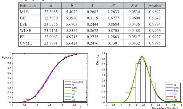
The results of real data analysis for gauge lengths data are given in tab. 3. Also, cdf and pdf curves of these estimators for LKw(a, b) distribution are given in fig. 1.

Table 3. The parameter estimates and selection criteria statistics for gauge lengths data

Estimator a^ _b ^ _{A* W* K-S p-value} MLE 22.3085 5.4072 0.2687 1.2633 0.0534 0.9892 BE 22.5930 5.3970 0.3119 1.6777 0.0600 0.9647 LSE 23.5756 5.6703 0.2444 0.8684 0.0436 0.9994 WLSE 23.7161 5.8354 0.2672 0.8705 0.0488 0.9966 PE 22.0063 4.9715 0.2735 1.2863 0.0517 0.9927 CVME 23.7881 5.6424 0.2476 0.7391 0.0432 0.9995 1 1.5 2 2.5 3 3.5 4 0 0.1 0.2 0.3 0.4 0.5 0.6 0.7 0.8 0.9 1 x F x( ) Empirical CDF PE CVME WLSE LSE BE MLE 0 0.5 1 1.5 2 2.5 3 3.5 4 4.5 5 0 0.1 0.2 0.3 0.4 0.5 0.6 0.7 0.8 0.9

Gauge lengths data

D e n si ty PE CVME WLSE LSE BE MLE

Figure 1. The curves for gauge lengths data; (a) cdf, (b) density

(for color image see journal web site)

Carbon fibers (in Gba) data

The second data set consists of 50 observations on breaking stress of carbon fibers (in Gba) obtained by Nichols and Padgett [33] is as follows:

3.70, 2.74, 2.73, 2.50, 3.60, 3.11, 3.27, 2.87, 1.47, 3.11, 4.42, 2.41, 3.19, 3.22, 1.69, 3.28, 3.09, 1.87, 3.15, 4.90, 3.75, 2.43, 2.95, 2.97, 3.39, 2.96, 2.53, 2.67, 2.93, 3.22, 3.39, 2.81, 4.20, 3.33, 2.55, 3.31, 3.31, 2.85, 2.56, 3.56, 3.15, 2.35, 2.55, 2.59, 2.38, 2.81, 2.77, 2.17, 2.83, 1.92.

The parameter estimates, and some selection statistics for carbon fibres data set are given in tab. 4.

Table 4. The parameter estimates and selection criteria statistics for carbon fibres data

Estimator a^ _b ^ _A* _W* _{K-S p-value} MLE 28.4793 3.1609 0.5142 1.9442 0.0845 0.8673 BE 28.0556 3.1329 0.5546 2.2357 0.0813 0.8959 LSE 35.3256 4.7092 0.5545 0.9684 0.0757 0.9369 WLSE 34.8359 4.6324 0.5531 0.9705 0.0790 0.9138 PE 26.8687 2.8253 0.5960 2.4165 0.0984 0.7182 CVME 35.7719 4.6719 0.5395 0.7860 0.0643 0.9860

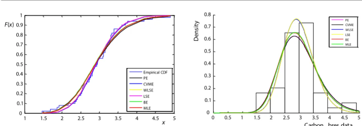
The cdf and pdf curves according to six different estimators are presented for carbon fibres data in fig. 2.

1 1.5 2 2.5 3 3.5 4 4.5 5 0 0.1 0.2 0.3 0.4 0.5 0.6 0.7 0.8 0.9 1 x F x( ) Empirical CDF PE CVME WLSE LSE BE MLE 0 0.5 1 1.5 2 2.5 3 3.5 4 4.5 5 0 0.1 0.2 0.3 0.4 0.5 0.6 0.7 0.8

Carbon bres data

D e n si ty PECVME WLSE LSE BE MLE

Figure 2. The curves for carbon fibres data; (a) cdf, (b) density

(for color image see journal web site) Concluding remarks

It has been considered ML, B, LS, WLS, P, and CVM estimation methods to estimate unknown parameters of LKw(a, b) distribution. Then, it is performed a Monte-Carlo simulation study to compare the performances of these estimators in terms of biases and MSE at different size of samples. According to results of simulation study, it is clearly seen that approximate bayes estimator is best the estimator among all estimators. Besides, as size of samples in-creases, biases and MSE of all estimators decrease. Also, it is seen that the biases and MSE of maximum likelihood estimators and approximate Bayes estimators approach each other in big size of samples. On the other hand, we illustrate usefulness of LKw(a, b) distribution for gauge lengths and carbon fibers data sets. Further, it is compared the fits of these estimators for LKw(a, b) distribution via Anderson-Darling, Cramer-Von Mises, Kolmogorov-Smirnov statis-tics and its p-values. It is seen that least square estimator is the best for gauge lengths data ac-cording to tab. 3. Approximate bayes estimator is the better than other estimators in modelling carbon fiber data according to tab. 4.

References

[1] Lemonte, A. J., et al., The exponentiated Kumaraswamy Distribution and Its Log-Transform, Brazilian

Journal of Probability and Statistics, 27 (2013), 1, pp. 31-53

[2] Kumaraswamy, P., A Generalized Probability Density Function for Double-Bounded Random Processes,

Journal of Hydrology, 46 (1980), 1-2, pp. 79-88

[3] Mohammed, H. F., Inference on the Log-Exponentiated Kumaraswamy Distribution, International

Jour-nal of Contemporary Mathematical Sciences, 12 (2017), 4, pp. 165-179

[4] Chacko, M., Mohan, R., Estimation of Parameters of Kumaraswamy-Exponential Distribution un-der Progressive Type-II Censoring, Journal of Statistical Computation and Simulation, 87 (2017), 10, pp. 1951-1963

[5] Akinsete, A, et al., The Kumaraswamy-Geometric Distribution, Journal of Statistical Distributions and

Applications, 1 (2014), Nov., 17

[6] Jose, K. K., Varghese, J., Wrapped Log Kumaraswamy Distribution and its Applications, International

Journal of Mathematics And Computer Research, 6 (2018), 10, pp. 1924-1930

[7] Korkmaz, M. C., Genc, A. I., Two-Sided Generalized Exponential Distribution, Communications in

Sta-tistics-Theory and Methods, 44 (2015), 23, pp. 5049-5070

[8] Korkmaz, M. C., Genc, A. I., A Lifetime Distribution Based on a Transformation of a Two-Sided Power Variate, Journal of Statistical Theory and Applications, 14 (2015), 3, pp. 265-280

[9] Ramos, P. L., Louzada, F., The Generalized Weighted Lindley Distribution: Properties, Estimation, and Applications, Cogent Mathematics, 3 (2016), 1, 1256022

[10] Dey, S., et al., Comparisons of Methods of Estimation for the NH Distribution, Annals of Data Science,

[11] Dey, S., et al., Kumaraswamy Distribution: Different Methods of Estimation, Computational and Applied

Mathematics, 37 (2018), 2, pp. 2094-2111

[12] Dey, S., et al., Statistical Properties and Different Methods of Estimation of Gompertz Distribution with Application, Journal of Statistics and Management Systems, 21 (2018), 5, pp. 839-876

[13] Ramos, P., et al., The Frechet distribution: Estimation and Application an Overview, On-line first, arXiv preprint arXiv:1801.05327, 2018

[14] Balakrishnan, N., Kundu, D., Birnbaum‐Saunders Distribution: A Review of Models, Analysis, and Ap-plications, Applied Stochastic Models in Business and Industry, 35 (2019), 1, pp. 4-49

[15] Tierney, L., Kadane, J. B., Accurate Approximations for Posterior Moments and Marginal Densities,

Jour-nal of the american statistical association, 81 (1986), 393, pp. 82-86

[16] Danish, M. Y., Aslam, M., Bayesian Estimation for Randomly Censored Generalized Exponential Dis-tribution under Asymmetric Loss Functions, Journal of Applied Statistics, 40 (2013), 5, pp. 1106-1119 [17] Gencer, G., Saracoglu, B., Comparison of Approximate Bayes Estimators under Different Loss Functions

for Parameters of Odd Weibull Distribution, Journal of Selcuk University Natural and Applied Science, 5 (2016), 1, pp. 18-32

[18] Kumar, K., Classical and Bayesian Estimation in Log-Logistic Distribution under Random Censoring,

International Journal of System Assurance Engineering and Management, 9 (2018), 2, pp. 440-451

[19] Kinaci, et al., Kesikli Chen Dağılımı için Bayes Tahmini (in Turkish), Selçuk Üniversitesi Fen Fakültesi

Fen Dergisi, 42 (2016), 2, pp. 144-148

[20] Tanis, C., Saracoglu, B.,. Statistical Inference Based on Upper Record Values for the Transmuted Weibull Distribution, International Journal of Mathematics and Statistics Invention, 5 (2017), 9, pp. 19-23 [21] Jung, M., Chung, Y., Bayesian Inference of Three-Parameter Bathtub-Shaped Lifetime Distribution,

Com-munications in Statistics-Theory and Methods, 47 (2018), 17, pp. 4229-4241

[22] Kao, J. H. K., Computer Methods for EstimatingWeibull Parameters in Reliability Studies, Trans IRE

Reliab Qual Control, 13 (1958), July, pp. 15-22

[23] Kao, J. H. K., A Graphical Estimation of Mixed Weibull Parameters in Life Testing Electron Tubes,

Tech-nometrics, 1 (1959), 4, pp. 389-407

[24] Gupta, R. D., Kundu, D., Generalized Exponential Distribution: Different Method of Estimations, Journal

of Statistical Computation and Simulation, 69 (2001), 4, pp. 315-338

[25] Alkasabeh, M. R, Raqab, M. Z., Estimation of the Generalized Logistic Distribution Parameters: Compar-ative Study, Statistical Methodology, 6 (2009), 3, pp. 262-279

[26] Erisoglu, U., Erisoglu, M., Percentile Estimators for Two-Component Mixture Distribution Models, Irani-an Journal of Science Irani-and Technology, TrIrani-ansactions A: Science, 43 (2019) 2, pp. 601-619

[27] Luceno, A., Fitting the Generalized Pareto Distribution Data Using Maximum Goodness-of-Fit Estima-tors, Computational Statistics and Data Analysis, 51 (2006), 2, pp. 904-917

[28] Macdonald, P., An Estimation Procedure for Mixtures of Distribution, Journal of the Royal Statistical

Society. Series B (Methodological), 30 (1968), 3 pp. 444-460

[29] Bader, M. G., Priest, A. M., Statistical Aspects of Fibre and Bundle Strength, in Hybrid Composites, in:

Progress in Science and Engineering of Composites, (Eds. T. Hayashi, K. Kawata, S. Umekawa), Japan

Society for Composite Materials, Tokyo, 1982, pp. 1129-1136

[30] Kundu, D., Raqab, M. Z., Estimation of R = P (Y < X) for Three-Parameter Weibull Distribution, Statistics

and Probability Letters, 79 (2009), 17, pp. 1839-1846

[31] Ghitany, M. E., et al., Power Lindley Distribution and Associated Inference, Computational Statistics and

Data Analysis, 64 (2013), Aug., pp. 20-33

[32] Nofal, Z. M., et al., The Generalized Transmuted-G Family of Distributions, Communications in Statistics – The-

ory and Methods, 46 (2017), 8, pp. 4119-4136

[33] Nichols, M. D., Padgett, W. J., A Bootstrap Control Chart for Weibull Percentiles, Quality and Reliability

Engineering International, 22 (2006), 2, pp. 141-151

Paper submitted: April 11, 2019 Paper revised: July 25, 2019 Paper accepted: August 1, 2019

© 2019 Society of Thermal Engineers of Serbia Published by the Vinča Institute of Nuclear Sciences, Belgrade, Serbia. This is an open access article distributed under the CC BY-NC-ND 4.0 terms and conditions