Intergenerational income mobility: Equality of opportunity a comparison of East and West Germany

INTERGENERATIONAL INCOME MOBILITY: EQUALITY OF OPPORTUNITY A COMPARISON OF EAST AND WEST GERMANY

BERNA FALAY 103622007

ĐSTANBUL BĐLGĐ ÜNĐVERSĐTESĐ SOSYAL BĐLĐMLER ENSTĐTÜSÜ EKONOMĐ YÜKSEK LĐSANS PROGRAMI

DOÇ. DR. EGE YAZGAN 2007

INTERGENERATIONAL INCOME MOBILITY: EQUALITY OF OPPORTUNITY A COMPARISON OF EAST AND WEST GERMANY

KUŞAKLARARASI FIRSAT EŞĐTLĐĞĐ: DOĞU VE BATI ALMANYA KARŞILAŞTIRMASI

BERNA FALAY 103622007

DOÇ. DR. EGE YAZGAN: ……….….. PROF. DR. REMZI SANVER: ……….. YRD. DOÇ. DR. KORAY AKAY: ……… TEZĐN ONAYLANDIĞI TARĐH: ………..

Toplam Sayfa Sayisi: 31

Anahtar Kelimeler: 1) Gelir hareketliliği 2) Boyut dönüşüm matrisleri 3) Fırsat eşitliği Keywords: 1) Income mobility 2) Size transition matrices 3) Opportunity of equality

ÖZET

Bu çalışmada kuşaklararası gelir hareketliliğinin Doğu ve Batı Almanya datası kullanılarak karşılaştırmalı analizi yapıldı. Gelir hareketliliği, fırsat eşitliği ve toplum refahı açısından incelendi. Bu anlayışı kullanan iki kısmi sıralama kullanıldı. Bunlardan biri Benabou-Ok sıralaması, diğeriyse Atkinson-Dardanoni sıralamasıdır. Almanya datası 1992-2005 aralığındaki baba-oğul ikililerini kapsar. Bu çalışmanın sonucunda, önceki çalışmalardan farklı olarak Batı Almanya erkek çocuklarının Doğu Almanya’da ki erkek çocuklarından daha eşit fırsatlarla karşılaşmakta olduğu ve gelirlerini uzun zamanda eşitlendiği gösterildi.

ABSTRACT

This paper examines the intergenerational income mobility in East and West Germany after reunification. Mobility is viewed as an opportunity equalizing and welfare enhancing concept. The two relevant partial orderings are used to evaluate these approaches, both are defined and used for the analysis of the data. The data consists of father-son pairs from panel data between the years 1992 and 2005. Size transition matrices are used for the results and they show that the Western states have a better opportunity equalizing income mobility process compared to the Eastern states according to Benabou-Ok ordering. In addition, it reveals that the West Germany mobility pattern is more welfare enhancing than the East Germany according to Atkinson-Dardanoni

TABLE OF CONTENTS

1. Introduction page 01

2. Partial orderings 04

2.1 Why size transition matrices? 04

2.2 Preliminaries 05

2.3 Opportunity of Equality 07

2.4 Atkinson- Dardanoni Ordering 09 3. Data and Earlier Studies on Germany 11

4. Empirical Application 13

5. Summary and Conclusion 25

6. Appendix 28

LIST OF TABLES

Table 4.1: Sample Characteristics for East page 13 Table 4.2: Sample Characteristics for West page 16 Table 4.3: Benabou-Ok dominance condition page 20 Table 4.4: Reynolds-Smolensky index of residual progressivity page 20

LIST OF GRAPHS

Graph 4.1: Age distribution for fathers, East page 14 Graph 4.2:Age distribution for sons, East page 14 Graph 4.3: Income distribution for fathers, East page 15 Graph 4.4: Income distribution for sons, East page 15 Graph 4.5: Age distribution for fathers, West page 16 Graph 4.6: Age distribution for sons, West page 17 Graph 4.7: Income distribution for fathers, West page 17 Graph 4.8: Income distribution for sons, West page 18

LIST OF FIGURES

Figure 4.1: Lorenz Curves for fathers’ and sons’ incomes in East Germany page 13 Figure 4.2: Lorenz Curves for fathers’ and sons’ incomes in East Germany

LIST OF TABLES

Table 4.1: Sample Characteristics for East page 13 Table 4.2: Sample Characteristics for West page 16 Table 4.3: Benabou-Ok dominance condition page 20 Table 4.4: Reynolds-Smolensky index of residual progressivity page 20

LIST OF GRAPHS

Graph 4.1: Age distribution for fathers, East page 14 Graph 4.2:Age distribution for sons, East page 14 Graph 4.3: Income distribution for fathers, East page 15 Graph 4.4: Income distribution for sons, East page 15 Graph 4.5: Age distribution for fathers, West page 16 Graph 4.6: Age distribution for sons, West page 17 Graph 4.7: Income distribution for fathers, West page 17 Graph 4.8: Income distribution for sons, West page 18

LIST OF FIGURES

Figure 4.1: Lorenz Curves for fathers’ and sons’ incomes in East Germany page 13 Figure 4.2: Lorenz Curves for fathers’ and sons’ incomes in East Germany

1. Introduction

It has been accepted that static snapshots of income distributions alone are not sufficient for meaningful evaluation of welfare. Not only one should focus on how incomes are distributed among individuals over a given period of time, one should also concern about how individuals’ incomes change over time. While the measurement of the former is an established concept, there is no consensus on the measurement of the income mobility.1 This may be because the notion of income mobility is not well-defined; different studies concentrate on different aspects of this multi-dimensional concept. Many different approaches are surveyed by Fields and Ok (1999a).

Intergenerational mobility is concerned with the correlation between the socio economic status of parents and the economic outcomes of their children when they become adults. Concluding that there is a strong relation between incomes across generations leads to a weak intergenerational mobility, and this leads to a violation of the norms of equality of opportunity and warrants government intervention. Therefore, the question of whether income inequality is transmitted to the next generation is at the hearth of many policy debates. It is for this purpose that mobility measure has to take into account of the welfare of the society as a whole, not the relative or the absolute changes of incomes of individuals.

Some researches view mobility as a relative concept in which the individuals of the society only changes their income positions [e.g. Prais (1955), Shorrocks (1978)]. Some

1

See Kolm (1960), Atkinson (1970), Dasgupta, Sen and Starett (1973) for details on the measurement of income inequality.

other researchers argue that mobility is an absolute concept where mobility rises once individuals move away from their initial income levels [e.g. Fields and Ok (1996,1999b)]. This paper’s approach of assessing mobility is more closely related to the papers, which take a welfare based view, such as Kanbur and Stiglitz (1986), and Dardanoni (1993)2. Mobility is of interest not because the movements of income dynamics is important, they may be equalizing or not but because it measures the extent to which longer-term incomes are distributed more or less equally than are single-year incomes. Therefore, mobility indices have been developed and been interpreted as indicators of "opportunity". For this reason, this paper views mobility as an equalizer of opportunities, not necessarily of outcomes. This point of view gives us the chance to get rid of measures that are only measuring the movements of individuals’ income without taking care of equalization through time.

The social welfare would certainly depend on the dynamics of income distribution and with the availability of the panel data these dynamics are utilized in procedures for testing mobility. A significant part of the literature on income mobility measurement uses “transition matrices” rather than distributional transformations. They are mainly useful devices for summarizing the mobility content of distributional transformations. In fact, they provide a summary of the movement of individuals among specified income classes. It is for this reason that transition matrices are used to determine the equalization of opportunity in this study.

2

See the important works of Shorrocks (1978a) and Maasoumi and Zandvakili (1986) for more welfarist income mobility measurement techniques.

On the other hand, it is worth to mention that some of the empirical work in the literature focused on the estimation of β in the following regression;

i father i son i y y₁ =β ₀ +ε (1)

where y₁son_i is the income of the adult son, and y₀father_i is the income of the father, i represents the family,

ε

_i is the error term. In this setup,

β

denotes the intergenerational correlation between y_0iandy_1i.

β

=0 represents a case of perfect mobility where the incomes are uncorrelated and

β

=1 as the perfect immobility where they are perfectly correlated.3 Solon (1992) estimated

β

ˆ as .41 using data from the Panel Study of Income Dynamics, which was considerably larger than .2 which was estimated by Becker and Tomes (1986). Aside from the econometric problems such as sample homogeneity and measurement error problems in these studies, the interpretation of

β

ˆ is ambiguous. As mentioned before, what really matters for the welfare of the society is not a result that can be concluded with this interpretation.

The purpose of this paper is to test equality of opportunity with transition matrices using panel data from Germany. While constructing the matrix, the rows are categorized according to the income classes, they may well be defined for different generations, intragenerational mobility or within the same generation, intergenerational mobility. This paper uses intergenerational mobility.

3

The remainder of the paper is organized as follows. Section 2 discusses two partial orderings that are used for the measurement of mobility processes which are Atkinson-Dardanoni and Benabou-Ok. Section 3 gives details of the data and some previous empirical studies. In section 4 results are given in detail. Section 5 concludes.

2. Partial Orderings

2.1 Why size transition matrices?

As discussed by Benabou-Ok (2001), income mobility cannot be evaluated independently of the values taken by income. When transition matrices are used to present a mobility process of a country, the coefficients represent the frequencies of transitions between income levels but assuming that the same transition probabilities are valid for different income levels, which is a difficulty of any analysis based on transition matrices. The real movements can not be fully represented by a discrete transition process. The alternative to this is the interfractile matrices which lead to another difficulty. For example, to be able to move from the 1st decile to the 2nd decile, one may need to double his income whereas to move from the 2nd decile to the 3rd decile may only mean to increase 15% of his income4. For these reasons, the measurement of the mobility should not depend only on the transition matrix but also on the income levels.

4

The types of matrices that are used to evaluate the opportunity of inequality are size transition matrices5. In this method, not only the boundaries between income classes are set exogenously but also they do not depend on the income regime. It reflects income movement between different income classes and this allows us to follow both the exchange of positions of the individuals and the economic growth. One can inspect the availability of the high-income positions. Welfare implications of mobility can be drawn, simply by comparing the matrices.

2.2 Preliminaries

Let x∈ ,

[

0 ∞

)

and y∈ ,

[

0 ∞

)

be two income variables with a continuous cumulative density functionM(x,y). The function M(x,y) is a function, which identifies a movement from income x to income y . This movement can be intergenerational if x is a father’s income and y is his son’s income or intragenerational if x and y are the incomes of the same individual at two points in time. For our purpose, the movement between xand y is described by a transition matrix, which is a transformation from a continuous cumulative density function of an income regime. As discussed in Section 2.1, in size transition matrices the boundaries are pre-determined.

Let n be the number of income classes in each income distribution with two different boundaries defined as 0<

α

₁ <

α

₂ <...<

α

_n−1 <∞ and

β

₁ <

β

₂ <...<

β

_n−1 <∞. The transition matrix P is denoted as P=

{ }

p_ij and each element p_ijof the matrix is a

5

conditional probability defining an individual with an initial class i of incomex moves to class j of income y , i.e.,

, ) Pr( ) and Pr( 1 1 1 i i j j i i ij x y x p

α

α

β

β

α

α

< ≤ < ≤ < ≤ = − − − with

α

₀ =

β

₀ =0 and

α

_n =

β

_n =∞.

A transition matrix is said to be monotone if an individual in income state i+1 has a better lottery over his future income than an individual in income state i, i.e.,

∑

= + ≥

∑

= k j k j i j j i p p 1 1, 1 , for all ,i k in {1,...,n−1

}

with strict inequality for some k.

And also let

π

_ibe the probability vector denoting the probability that an individual falls into class i of incomex, i.e.,

)

Pr( _{i 1 i}

ij

α

x

α

π

= ₋ ≤ <

In other words,

π

_iis the proportion of the people in the ith class of x and p is the _ij proportion of the people that moves to class j of income y, given that he was initially in class i of income x.

2.3 Opportunity of Equality

The notion of mobility as a mechanism that equalizes income opportunities but not necessarily of outcomes as in Benabou and Ok (2001) is a partial ordering which corresponds to the notion of progressivity similar to the one that is used to assess tax functions in public finance. Mobility is viewed as progressivity in the mapping between initial outcomes and future opportunities which should not only depend on the movements of each individual’s income through time but the sum of all expected income. A tax function maps pre-tax incomes to post-tax incomes whereas mobility process maps initial incomes to expected future incomes, like a stochastic redistribution. The measurement of the level of equality of opportunity is an application of the measurement of progressivity of the mapping in the sense of having decreasing average tax rates. The theory of progressivity measurement and Lorenz dominance can be applied.6 A mobility process is more equal than another one if it results in a higher Lorenz curve for the distribution of individual levels of intertemporal welfare. Assessing mobility as an equality of ex-ante opportunities is not the same as assessing the equality of ex-post outcomes like in Kanbur and Stromberg (1988) and Dardononi (1993). Future realized income distributions can be more unequal but this first and foremost reflects shocks, which were not predictable on the basis of initial conditions. Furthermore, the income distributions in different periods must overlap in the steady-state. These are the reasons why outcome-based comparisons can not be utilized for some cases. It is also worth to mention that standard mobility concepts and measures are in many cases inconsistent with mobility as an equalizer of longer-term incomes (Fields, 2005).

6

Benabou-Ok Theorem:

Let (

λ

₁,

λ

₂,...,

λ

_n) be the income vector associated with the n income classes with

n

λ

λ

λ

₁ < ₂ <...< in both regimes and let P and Q be two n ×n monotone transition

matrices. And let =

∑

n₌

j ij j i P p e 1 )

(

λ

λ

be the expected income of a person under the mobility process P initially in the ith class. The following statements are equivalent.

(i) P is more opportunity equalizing than Q for all possible income distributions: denoted as Pf_BO Q. (ii) ; ) ( ) ( ... ) ( ) ( 1 1 n Q n P Q P e e e e

λ

λ

λ

λ

≥ ≥ (iii) (D∗ −D_∗)

[

Pyy'Q'

]

≥0

where D denotes the first super-diagonal and * D_* denotes the first sub-diagonal of the matrix. Condition (ii) states that the expected incomes are equalized at a faster rate under the mobility process P than under the process Q . Condition (iii) is the operational equivalent of the ordering.

When P and Q can not be ranked according to > , one can use the difference between _BO the Gini coefficients which is equal to the area between the two Lorenz curves, namely the Reynolds-Smolensky (1997) index of residual progressivity:

) ( ) ( − −1 ≡ _M RS M Gini F Gini Foe

ρ

This gap increases as M increases in the mobility ordering _fBO.

2.4 Atkinson- Dardanoni Ordering

Atkinson (1983) proposed the first dominance approach to measuring income mobility, relating mobility with a social welfare function defined over incomes at different dates. In his approach mobility is again a concept whose welfare implications have to be investigated.

Atkinson- Dardanoni Theorem:

Let W(x,y) be a utilitarian social welfare function:

∫∫

∞ ∞ = 0 0 ) , ( ) , ( ) , (x y U x y dM x y W , (2)

where U(x,y) satisfies U_xy ≤0 and other regulatory conditions. For two income regimes, characterized by M(x,y) and N(x,y) with identical marginal distributions or the distribution is at steady-state, he showed that the regime with M(x,y) has greater social welfare than N(x,y) according to all W(x,y) if and only if

) , ( ) , (x y N x y

with strict inequality holding for some x and y . In matrix setup, for two transition matrices P and Q this inequality becomes

∑∑

∑∑

= = = = ≤ k i l j ij j k i l j ij jp q 1 1 1 1

π

π

for all k and kl, , l=1,...,m, (4)

with at least one strict inequality holding for some k and l which will be denoted as Q

Pf_AD . The condition of having equal marginal distributions is equivalent to the sums of rows and columns must be the same between the matrices. This is the dynamic equivalent of the static inequality ranking of income distributions by the Lorenz curve. Dardanoni (1993) also characterized condition (4) and showed that Atkinson’s condition is necessary and sufficient for one regime to have greater (Bergson–Samuelson) social welfare.

There is a duality between the orderings of Benabou-Ok and Atkinson-Dardanoni in the sense that both compare the expected future incomes under the mobility processes. But in contrast to the Atkinson-Dardanoni, Benabou-Ok’s condition does not require the initial income distributions to be equal or in other words a common steady-state. > is _BO conditional on income state vector holding for all income distributions while >_AD is conditional on a particular income distributions holding for all income state vectors.7

7

3. Data and Earlier Studies on Germany

The analysis of income mobility in Germany uses the German Socio-Economic Panel (GSOEP). The GSOEP is a longitudinal database with micro data that was obtained from annual face-to-face interviews of representative German households. It started in 1984 in the Federal Republic of Germany (FRG) and was extended to the area of the former German Democratic Republic (GDR) one month prior to German monetary union in July 1990. After German reunification it was continued separately in the eastern and western states of Germany. Since 1990, the GSOEP has been administered by the Deutsches Institut für Wirtschaftsforschung (DIW) in Berlin. For further information, see Wagner et al. (1993). All persons in household are to be surveyed also the following years at same address as well as after a residential move within Germany. Personal interviews start at age of 16. The household is followed until two consecutive temporary drop-outs of all household members or a final refusal. There are seven sub-samples8

This data is giving the researches the opportunity to analyze many questions in understanding the impact of reunification of Germany. After the monetary union, the East German Mark was replaced with the West German, Deutsche Mark (DM) at a one-to-one rate allowing us to compare incomes. And also there is a fact to keep in mind throughout the analysis that in 1990, there were no unemployment in the eastern states and in 1995 the rate was 16.9 percent. For western states it was 4.3 percent in 1990 and 7.5 percent in 1995. Since we are interested in the labor earnings this will induce a loss of income which will cause a downward mobility. (Hauser and Fabig, 1999)

8

For the purpose of this paper, the interest is to see if the mobility as an equalizer of opportunity in the eastern states of Germany is higher or lower as compared to the level of western states after reunification, asking which of these mobility processes better equalizes children’s –son’s for this particular study– opportunities, for any arbitrary distribution of parental backgrounds.

Mueller and Frick (1996) were one of the first to compare the income mobility in eastern and western states of Germany. After that, Couch and Dunn (1997) uses data from the Panel Study of Income Dynamics and GSOEP to estimate the intergenerational elasticity of earnings between fathers and sons of .11 for Germany and .13 for U.S. by using log annual earnings averaged over the period 1984-1989. And also their result indicates that there is remarkable similarity between the two countries in the correlations of earnings of fathers and sons.

Although intergenerational mobility comparison has been done to many market economies for different countries by many authors, there is no known income mobility study on a centrally planned socialist economy until Hauser and Fabig (1999). They used GSOEP between 1990 and 1995. They find that gross individual income mobility is much higher in the East than in the West during the first years after the reunification, but this difference has become much smaller until 1995.

The work of Fabig (1999) examines the gross and net equivalent income mobility in the western and eastern states of Germany, in Great Britain and in the United States, using

panel data of these countries between the years 1989-1995. The results show that the largest mobility-reducing effect of the welfare state –tax and transfer system– is observed in eastern states of Germany.

4. Empirical Application

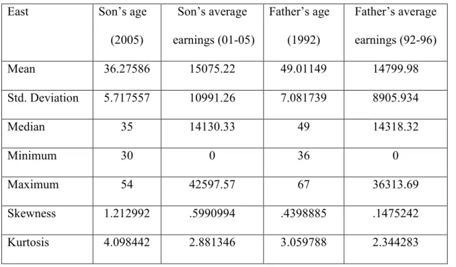
To compare opportunity of equality of fathers and sons in East and West Germany after reunification, father-son pairs are selected from employed/unemployed without any restriction. The main sample comprises 87 father-son pairs from East Germany and 389 father-son pairs from West Germany. The fathers in the sample are the household heads who, in the 1990 survey, had a son at the age of 15 or older. The reason for this restriction in the sample is to observe the earnings of the adult sons –at least 30 years old– in 2005. Earnings observed at younger ages would be noisy measures of long-run status. Fathers’ earnings are calculated as the average of 5-year earnings, years between 1992 and 1996. Likewise sons’ earnings are the average earnings of 5-year earnings, years between 2001 and 2005. The sons’ earnings are deflated accordingly. Table 4.1 presents some summary statistics on the age and average earnings of the main sample’s fathers and sons for the East and Table 4.2 presents the same statistics for the West9. As can be easily observed from Graph 4.1, 4.2, 4.5, and 4.6, East and West father-son pairs have the same age profile. The mean for the sons are 36 and the mean for the fathers are around 50 when their incomes are used as an indicator of their life-time earnings. While the fathers’ age distribution resembles more of a normal distribution around their mean 50, the sons’ age distribution is the right tale of the whole curve because of the age

9

Empirical results are based on calculations using Stata (Version 9.2), including the ado files ineqdeco5 and glcurve7.

restriction. Graph 4.3 and 4.4 display the incomes of the fathers and sons for the eastern states while Graph 4.7 and 4.8 display them for the western states. Because the sons are observed at an earlier stage of the life cycle, their mean earnings are lower compared to their fathers for both states and the standard deviation of their earnings is higher only for East. The distributional difference is that the earnings of the East data look more of a normal distribution while the incomes of the West data are similar to a Weibull distribution. The main difference between the profiles of the East and the West is the number of father-son pairs.

Table 4.1: Sample Characteristics for East

East Son’s age

(2005) Son’s average earnings (01-05) Father’s age (1992) Father’s average earnings (92-96) Mean 36.27586 15075.22 49.01149 14799.98 Std. Deviation 5.717557 10991.26 7.081739 8905.934 Median 35 14130.33 49 14318.32 Minimum 30 0 36 0 Maximum 54 42597.57 67 36313.69 Skewness 1.212992 .5990994 .4398885 .1475242 Kurtosis 4.098442 2.881346 3.059788 2.344283

0 .0 5 .1 .1 5 D e n s it y 30 40 50 60 70

Age Distribution Father-East

Graph 4.1: Age distribution for fathers, East

0 .0 5 .1 .1 5 D e n s it y 30 35 40 45 50 55

Age Distribution Son-East

0 1 .0 e -0 5 2 .0 e -0 5 3 .0 e -0 5 4 .0 e -0 5 D e n s it y 0 10000 20000 30000 40000

Income Distribution Father-East

Graph 4.3: Income distribution for fathers, East

0 1 .0 e -0 5 2 .0 e -0 5 3 .0 e -0 5 4 .0 e -0 5 D e n s it y 0 10000 20000 30000 40000

Income Distribution Son-East

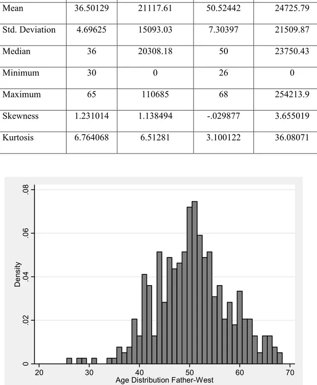
Table 4.2: Sample Characteristics for West

West Son’s age

(2005) Son’s average earnings (01-05) Father’s age (1992) Father’s average earnings (92-96) Mean 36.50129 21117.61 50.52442 24725.79 Std. Deviation 4.69625 15093.03 7.30397 21509.87 Median 36 20308.18 50 23750.43 Minimum 30 0 26 0 Maximum 65 110685 68 254213.9 Skewness 1.231014 1.138494 -.029877 3.655019 Kurtosis 6.764068 6.51281 3.100122 36.08071 0 .0 2 .0 4 .0 6 .0 8 D e n s it y 20 30 40 50 60 70

Age Distribution Father-West

Graph 4.5: Age distribution for fathers, West

0 .0 2 .0 4 .0 6 .0 8 D e n s it y 30 40 50 60 70

Age Distribution Son-West

Graph 4.6: Age distribution for sons, West

0 5 .0 e -0 6 1 .0 e -0 5 1 .5 e -0 5 2 .0 e -0 5 2 .5 e -0 5 D e n s it y 0 50000 100000 150000 200000 250000

Income Distribution Father-West

0 1 .0 e -0 5 2 .0 e -0 5 3 .0 e -0 5 4 .0 e -0 5 D e n s it y 0 20000 40000 60000 80000 100000

Income Distribution Son-West

Graph 4.8: Income distribution for sons, West

In constructing transition matrices, we use five earning classes in DM. The class boundaries are 0DM, 7000DM, 12500DM, 17000DM, 23000DM and ∞ . The representative income level of each class is assigned as the midpoint of that class so the income vector λ is (3500DM, 9750DM, 14750DM, 20250DM, 30000DM).

The distributions of fathers’ income within these classes in Eastern states are as

) 172 . 0 , 218 . 0 , 195 . 0 , 206 . 0 , 206 . 0 ( ˆ_EF =

π

) 503 . 0 , 161 . 0 , 06 . 0 , 04 . 0 , 218 . 0 ( ˆ_WF =

π

.

The distributions of sons’ incomes in 2001-2006 in Eastern states are as

) 172 . 0 , 218 . 0 , 218 . 0 , 103 . 0 , 287 . 0 ( ˆ_ES =

π

and in Western states

) 393 . 0 , 213 . 0 , 105 . 0 , 08 . 0 , 203 . 0 ( ˆ_WS =

π

.

The transition matrix over the period for East is

                = 0.400 0.267 0 0.133 0.200 0.158 0.105 0.211 0.053 0.474 0.176 0.294 0.412 0 0.118 0.167 0.111 0.278 0.167 0.278 0 0.333 0.167 0.167 0.333 ˆ P

and for West is

                = 0.383 0.184 0.102 0.092 0.240 0.365 0.222 0.127 0.079 0.206 0.407 0.148 0.111 0.148 0.185 0.333 0.278 0.222 0.056 0.111 0.447 0.282 0.071 0.059 0.141 ˆ Q .

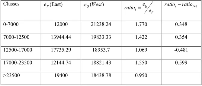
Both West and East Germany’s incomes are transformed by using the same income scale therefore both countries have the same income level for each income class. As a result, the equal income level requirement of the Benabou-Ok theorem is fulfilled. There is no assumption that the initial distributions to be the same as in Atkinson- Dardanoni ordering. Table 4.3 lists the expected incomes under each transition matrix. The last column has to be non-negative for the dominance to hold which is non-negative except one.

Table 4.3 – Benabou-Ok dominance condition

Classes e_P(East) e_Q(West)

P Q

i _e

e

ratio = ratioi −ratioi+1

0-7000 12000 21238.24 1.770 0.348

7000-12500 13944.44 19833.33 1.422 0.354

12500-17000 17735.29 18953.7 1.069 -0.481

17000-23500 12144.74 18821.43 1.550 0.599

>23500 19400 18438.78 0.950

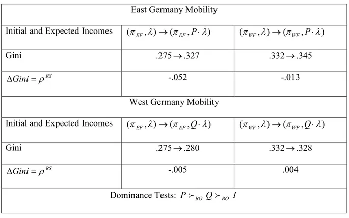
Their condition is not satisfied, therefore P and Q can not be ranked according to _fBO but still one can compare them according to Reynolds-Smolensky index of residual progressivity. The results are summarized in Table 4.4.

Table 4.4: Reynolds-Smolensky index of residual progressivity East Germany Mobility

Initial and Expected Incomes (

π

_EF,

λ

)→(

π

_EF,P⋅

λ

) (

π

_WF,

λ

)→(

π

_WF,P⋅

λ

)

Gini .275→.327 .332→.345

RS

Gini=

ρ

∆ -.052 -.013

West Germany Mobility

Initial and Expected Incomes (

π

_EF,

λ

)→(

π

_EF,Q⋅

λ

) (

π

_WF,

λ

)→(

π

_WF,Q⋅

λ

)

Gini .275→.280 .332→.328

RS

Gini=

ρ

∆ -.005 .004

Dominance Tests: Pf_BO Qf_BO I

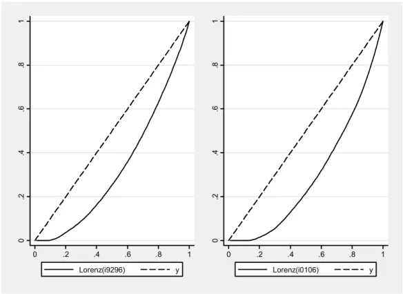
The very first thing to notice is that there is more cross-sectional inequality in Western states than Eastern states. As can be easily observed from the first graphs of Figure 4.1 and Figure 4.2, the West Lorenz curve for fathers’ incomes is everywhere below its East counterpart, with respective Gini coefficients G_WF =.332 and G_EF =.275. When we look at the degree that these differences in social origins determine the next generations’ opportunities, these two Lorenz curves for sons’ incomes can not be distinguished, with Gini coefficients G_WS =.328 and G_ES =.327. The corresponding indices of progressivity are

ρ

_WestRS =.004 and

ρ

_EastRS =−.052. Although this result means that the West is more opportunity equalizing than the East, however it can still not be considered as fair for there is less to equalize in the East. To be able to compare them, one has to work with the same initial income distribution. This means that starting with the East’s income

distribution, the West’s mobility process Q is applied and visa versa. If the West mobility process Q operated on the East’s distribution of fathers’ incomes, the Gini for sons’ opportunities would have been increased to –.005 which is more than –.052. And again if the East mobility process P operated on the West’s distribution of father’s incomes, the Gini would have changed to –.013. The first row of Table 4.4 reveals that mobility process of the West is unambiguously more egalitarian than the East, which contrasts with the outcomes.

0 .2 .4 .6 .8 1 0 .2 .4 .6 .8 1 Lorenz(i9296) y 0 .2 .4 .6 .8 1 0 .2 .4 .6 .8 1 Lorenz(i0106) y

Figure 4.1: Lorenz Curves for fathers’ and sons’ incomes in East Germany

0 .2 .4 .6 .8 1 0 .2 .4 .6 .8 1 Lorenz(i9296) y 0 .2 .4 .6 .8 1 0 .2 .4 .6 .8 1 Lorenz(i0106) y

The requirement of equal initial distributions between the two states in the Atkinson-Dardanoni condition is not satisfied because the sums of rows and columns are not the same between matrices P and Q. Instead of asking this broad question, the following question can be asked: If the West transition pattern is imposed on the East initial distribution, would the East earnings be equally mobile? The Atkinson-Dardanoni condition examines if the West transition matrix is equally welfare increasing as the East matrix.

{

∑ ∑

k_{= =} −

}

i l j j pij qij 1 1

π

( ) is                 0 0.218 0.218 0.133 0.107 -0 0.213 0.213 0.125 0.116 -0 0.170 0.163 0.075 0.060 -0 0.124 0.149 0.131 0.074 -0 0.092 0.082 0.062 0.040 -.

Thus, according to Benabou-Ok and Atkinson-Dardanoni orderings, West transition pattern equalizes and yields a greater social welfare than East transition pattern.

5. Summary and Conclusion

Equality of opportunity is the term by which public policy changes are often judged, and as a result there is a strong need for plausible indicators of the extent to which social institutions lead to fair outcomes. This is one of the principal reasons why the degree of intergenerational income mobility is viewed as being policy relevant. Therefore many studies have focused to understand why it is important.

This paper aimed to compare the two different economies, East and West Germany, which are initially a natural environment to compare the differences between a centrally-planned socialist economy and a market economy. This is the reason why it is interesting to see the impact of reunification of the two, from an intergenerational mobility

perspective.

The study was made possible through the availability of the panel data, GSOEP. From the vast amount of data available, father-son pairs were selected from the two states in order to do the comparison of income dynamics using two partial orderings: Benabou-Ok and Atkinson-Dardanoni. The two orderings both have agreed that the West’s mobility process is ambiguously better than the East’s. Not only it better equalizes the opportunities of the next generation but it also yields a greater social welfare. It is interesting to see that the previous studies with this data on the measurement of mobility have shown the opposite. The reason behind the contradicting results is that this paper is not viewing the mobility as a relative or an absolute measure but rather a concept that should be evaluated from a welfare-based approach. A mobility pattern is a better

equalizer of opportunities only if it equalizes the lifetime incomes of the whole society or if it is more progressive in the sense of having decreasing average tax rates.

The mobility patterns of the two could not be ranked using first the Benabou-Ok

ordering. Then again using a result of the same origin, initial income distributions of the two were switched and indices of progressivity were calculated. The results showed that the West Germany performed better in equalizing opportunities of incomes than the East Germany while the East’s mobility pattern performed worse with the West’s initial income distribution.

The requirement of the same initial income distributions of Atkinson-Dardanoni ordering could not be satisfied. Instead of asking the broad question of whether the East is more mobile in incomes than the West, the question was narrowed to: If West’s pattern is imposed upon the income distribution of the sons of the East would it then result in a higher welfare enhancing profile? The answer is again positive.

With little consensus on how mobility should be viewed and why it is important, this paper is an effort to understand its social welfare implications. Many other orderings can be utilized to see if these results are valid.

6. Appendix

Sub-sample details are as follows.

Sub Samples Started in No of Households

A. West-German 1984 4528 Head is either German or

other nationality than those in Sample B.

B. Foreigners 1984 1393 Head is either Turkish,

Italian, Spanish, Greek, or Yugoslavian.

C. East-Germans 1990 2179 Head was a citizen of the GDR.

D. Immigrants 1994/95 522 At least one HH member has

moved to Germany after 1984.

E. Refreshment sample

1998 1067 Random sample covering all

existing subsamples (total population)

F. Innovation sample

2000 6052 Random sample covering all

existing subsamples (total population)

G. High Income sample

2002 1224 Monthly net Household

income > 7.500 DM (4.500 EUR in wave 2)

7. References

Atkinson, A. B. (1970). On the measurement of Inequality. Journal of Economic Theory, 2, 244-263.

Atkinson, A. B. (1983). The measurement of economic mobility. Social Justice and Public Policy: Cambridge: MIT Press.

Becker, G. & Tomes N. (1986). Human capital and the rise and the fall of families. Journal of Labor Economics, 4, 1-39

Benabou, R. & Ok E. A. (2001). Mobility as progressivity: ranking income processes according to equality of opportunity. NBER, working paper 8431.

Couch, K. A. & Dunn, T. A. (1997). Intergenerational correlations in labor market status: A comparison of the Unites States and Germany. The Journal of European Social Policy, Vol. 32, No:1, 210-232

Dardanoni, V. (1993). On measuring social mobility. Journal of Economic Theory, 61, 372-394.

Dasgupta, P., Sen, A. and Starett, D. (1973). Notes on the measurement of inequality. Journal of Economic Theory, 6(2), 180-187.

Fellman, J. (1976). The effect of transformation on Lorenz curves. Econometrica, 44, 823-4.

Fabig, H. (1999). Income mobility and the welfare state: an international comparison with panel data. Journal of Economic Social Policy, Vol. 9, No:4, 331-349. Fields, G. (2005). Does income mobility equalize longer-term incomes? New Measures

Fields, G. & Ok, E. A. (1996). The meaning and measurement of income mobility. Journal of Economic Theory, 71, 349 –377.

Fields, G. & Ok, E.A. (1999a). The measurement of income mobility: an introduction to the literature. Handbook of Inequality Measurement, ed.by J. Silber, Dordrecht, Kluwer Academic Publishers, 557-596.

Fields, G. & Ok, E.A. (1999b). Measuring movement of incomes. Economica, 66, 455- 471.

Formby, J., Smith, J. & Zheng B. (2004). Mobility measurement, transition matrices and statistical inference. Journal of Econometrics, 120, 181-205.

Haisken-DeNew, J. & Hahn M. (2006). Panelwhiz: A flexible modularized Stata interface for assessing large scale panel data sets. mimeo.

Hauser, R., Fabig, H. (1999). Labor earnings and household income mobility in reunified Germany: A comparison of the Eastern and Western states. Review of Income and Wealth (45) Number 3, 303-324.

Hungerford, T. L. (1993). U.S. income mobility in the seventies and eighties. Review of Income and Wealth, 31(4), 403-417

Jakobsson, U. (1976). On the measurement of the degree of progressivity. Journal of Public Economics, 5, 161-168.

Kanbur, R. and Stiglitz, J. (1986). Intergenerational mobility and dynastic inequality. Princeton Woodrow Wilson School Discussion Paper in Economics: 111. Kanbur, R. and Stromberg, J-O. (1998). Income transitions and Income Distribution

Dominance. Journal of Economic Theory 45, 408-416.

Kolm, S. C. (1960) The optimal production of justice. Public Economics, J. Margolis and H, Guitton eds., MacMillan: London

Maasoumi E. & Zandvakili S. (1986) A class of generalized measures of mobility with applications. Economic Letters Volume 22, Issue 1, 97-102

Mueller, K. & Frick, J. (1996). Die Einkommensmobilitaet

(Nettoaequivalenzeinkommen) in den neuen und alten Bundeslaendern 1990-94, in S. Hrardil and E. Pankoke (eds.), Aufstieg fuer alle?,KSPW Beitraege zum Bericht Ungleichheit und Sozialpolitik, Band 2.2, Leske & Budrich, Opladen. Prais, S. J. (1955). Measuring social mobility. Journal of the Royal Statistical Society

Series A (Part I), 118, 56–66.

Reynolds, M. & Smolensky, E. E. (1977). Public expenditures, taxes and the distribution of income: The United States 1950, 1961, 1970. New York: Academic Press. Shorrocks, A. F. (1978a). The measurement of mobility. Econometrica 46,1013 –1024. Shorrocks, A. F. (1978b). Income inequality and income mobility. Journal of Economic

Theory, Volume 19, Issue2, 376-393

Solon, G. (1999). Intergenerational mobility in the labor market. Handbook of Labor Economics, Volume 3, Part1, 1761-1800

Wagner, G., Burkhauser, R. and Behringer, F. (1993) The English Language Public Use File of the German Socio-economic Panel, Journal of Human Resources 28: 429-33.