Selçuk J. Appl. Math. Selçuk Journal of Vol. 8. No.2. pp. 57 - 69 , 2007 Applied Mathematics
On Total Number Of Candidate Component Cluster Centers And To-tal Number of Candidate Mixture Models In Model Based Clustering
Tayfun Servi and Hamza Erol
Çukurova University, Faculty of Arts and Sciences, Department of Statistics, 01330 Adana — Turkey;
e-mail:tservi@ cu.edu.tr , herol@ m ail.cu.edu.tr
Received : August 23, 2007
Summary. Determining the number of component clusters for a multivariate normal mixture model is the most important problem in model based clustering and determining the number of candidate mixture models is the most interest-ing problem in multivariate normal mixture model based clusterinterest-ing usinterest-ing model selection criteria. In this study; first, the concept of the total number of can-didate component cluster centers is introduced and an interval is constructed by using the number of partitions in each variable in multivariate data. Sec-ond, an equation is given for the total number of candidate mixture models in multivariate normal mixture model based clustering. The number of candidate mixture models is defined as the sum of the number of possible mixture models with different number of component clusters.
Key words: Multivariate normal mixture model, Mixture model based clus-tering, Model selection, Total number of candidate component cluster centers, Total number of candidate mixture models, Number of possible mixture models. Mathematics Subject Classification (2000): 91C20, 62H30.
1. Introduction
There are several clustering methods for partitioning of -dimensional multi-variate data into meaningful subgroups. One of them is the multimulti-variate normal mixture model based clustering. Multivariate normal mixture model based clus-tering is one way of partitioning -dimensional multivariate data into meaning-ful groups or clusters [1]. Each component of the multivariate normal mixture model corresponds to a cluster. Multivariate normal mixture models provide powerful tools for density estimation, clustering and discriminant analysis. Mul-tivariate normal mixture models are used for modelling a wide variety of random phenomena [2]
Multivariate mixture model based clustering assumes a set of -dimensional vectors 1 of observations from a multivariate mixture of a finite number of groups or clusters each with some unknown proportions 1 . It is assumed that the multivariate mixture density of the th data point for = 1 can be written as (1) (; ) = X =1 (; )
where denotes the mixing proportion of the data points in group or cluster such that 0 1 and
P =1
= 1 . The group conditional densities (; ) depend on an unknown parameter vector [3]. (; )’s are assumed to be multivariate normal group conditional densities, with mean vector and covariance matrix Σ, of the form
(2) (; ) = 1 (2)2|Σ| 1 2 exp ½ −12( − )Σ−1 ( − ) ¾
where ’s are the vectors of parameters in the component densities, thus = ( Σ). The superscript denotes the transpose. So = (1 1 ) denotes the vector of all unknown parameters in the multivariate normal mix-ture model over the parameter space Ω.
Fraley and Raftery [4] studied the problem of determining the structure of clus-tered data, without prior knowledge of the number of clusters or any other infor-mation about their composition. McLachlan and Chang [5] considered cluster analysis via finite mixture model approach in medical research. Recently, Gal-imberti and Soffritti [6] used model based methods to identify multiple cluster structures in a data set. They used partitioning variables approach to clus-tering. The mixture modeling (MIXMOD) program fits mixture models to a given data set for the purposes of density estimation, clustering or discriminant analysis [7].
Fraley and Raftery [4] defined the model based strategy for model based clus-tering. The strategy for model based clustering starts with determination of a maximum number of clusters. But there is no any criteria for “the deter-mined maximum number of clusters” yet. All parameters in the multivariate normal mixture model are estimated by the maximum likelihood method using together with the Expectation and Maximization (EM) algorithm [8], the Sto-chastic EM (SEM) algorithm [9] and the Classification EM (CEM) algorithm [10], and information criterias are computed for each mixture model from two to the determined maximum number of clusters. This leads unnecessary operations in algorithms used for clustering. The best clustering model can be obtained by using several information criterions. Among them, Akaike’s information crite-rion (AIC) [11] and the Bayesian information critecrite-rion (BIC) [12] are most well
known. The mixture model that minimizes the AIC value is taken as the opti-mum model. The AIC tends to overestimate the number of component clusters [3], but it is still often used in practice. In comparison to the AIC, the BIC will select mixture models with fewer parameters (at least for cases where 8). Although certain regularity conditions used in the derivation of the measure in practice will not be satisfied, this measure has appeared to work very well. There are two main purposes of this study. First, the total number of candidate component cluster centers ( ) is defined and an interval is constructed by using the number of partitions in each variable in multivariate data, since the mixture structure of each variable forms the candidate component cluster centers in multivariate data. Component cluster centers occur at these candidate component cluster centers. This idea will be explained in Section 2. Second, an equation is given for the total number of candidate mixture models ( ) in multivariate normal mixture model based clustering using model selection criteria [13]. The number of candidate mixture models ( ) is defined as the sum of the number of possible mixture models ( ) with different number of component clusters. The best or optimum model is chosen among these possible mixture models. The and the can be very important in finding the optimum or the best model. This idea will be explained in Section 3. The approach, in this study, can lead a genetic algorithm for the multivariate normal mixture model clustering of multivariate data, but this is not in the scope of this study. This may be a subject of another study.
This paper is organized as follows. In Section 2, an interval is constructed for the . An equation will be given for the in Section 3. Some applications of the interval constructed for the in multivariate normal mixture model clustering is given in Section 4. Finally some conclusions and remarks are given in Section 5.
2. An Interval For The Total Number Of Candidate Component Clus-ter CenClus-ters In Multivariate Normal Mixture Model Based ClusClus-tering Identification of multiple cluster structures in -dimensional multivariate data is an interesting problem in mixture model based clustering. Soffritti [14] de-veloped model based procedures for detecting multiple cluster structures from independent subset of variables. An approach combining the model based pro-cedure with variable clustering method is proposed by Galimberti and Soffritti [6].
The interval for the can be obtained by partitioning each variable in -dimensional multivariate data since the mixture structure of each variable forms the component clusters in -dimensional multivariate data. Let’s consider the mixture structure of each independent variable in -dimensional multi-variate data for = 1 . Let’s assume that the observed data 1 has the multivariate normal mixture model in equation (1) with component densities in equation (2). The variable in -dimensional multivariate data is classified into one of two classes in this study by
(3) = ⎧ ⎪ ⎪ ⎨ ⎪ ⎪ ⎩
with 1, if have a mixture structure (Thus, univariate normal mixture case) with = 1, if have not a mixture structure
(Thus, univariate normal case)
⎫ ⎪ ⎪ ⎬ ⎪ ⎪ ⎭ where denote the number of components of the variable in -dimensional multivariate data. The connection between th observation and th variable in -dimensional multivariate data can be defined by . Here, denotes the th observation of the th variable in -dimensional multivariate data. Then the interval for the can be obtained by
(4) max {1 } ≤ ≤ Y =1
for the multivariate normal mixture model with component clusters of -dimensional multivariate data. In equation (4), {1 } is the mini-mum of the total number of candidate component cluster centers, thus min= max {1 } and
Y =1
is the maximum of the total number of candidate
cluster centers, thus max= Y =1
.
The logic of and maxwill be explained on an example for 2-dimensional multivariate data, thus bivariate normal mixture model. Let 1 = 2 for 1 and 2 = 2 for 2 in 2-dimensional multivariate data. For the case considered, min= max {2 2} = 2 and max= 12 = 22 = 4.
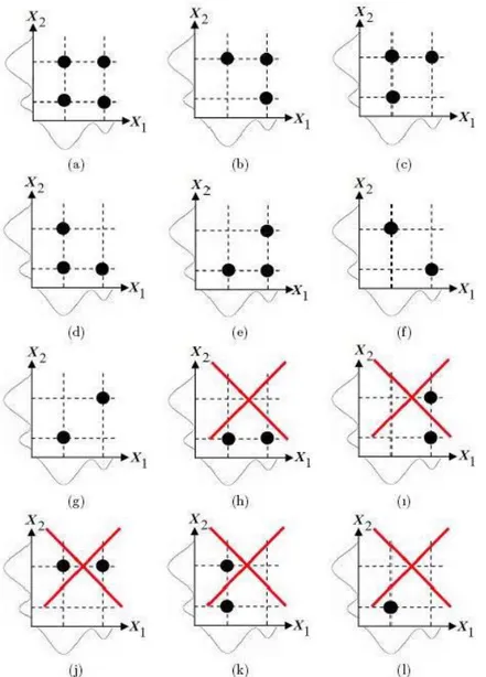
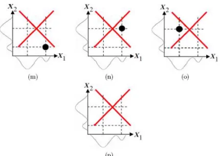
The bivariate normal mixture model for the case considered can have only one bivariate normal mixture model with at most 4 component clusters when the number of candidate component cluster centers is 4. This is the case (a) in Figure 1. The bivariate normal mixture model for the case considered can have four bivariate normal mixture model with 3 component clusters when the number of candidate component cluster centers is 3. These are the cases (b)-(e) in Figure 1. The bivariate normal mixture model for the case considered can have six bivariate normal mixture model with 2 component clusters when the number of candidate component cluster centers is 2. These are the cases (f)-(k) in Figure 1. The cases (f) and (g) in Figure 1 are possible. The cases (h) and (j) in Figure 1 are impossible since 2= 1 in cases (h) and (j) and this contradicts with the assumption 2 = 2. The cases (i) and (k) in Figure 1 are impossible since 1= 1 in cases (i) and (k) and this contradicts with the assumption 1= 2. The bivariate normal mixture model for the case considered can not have any of four bivariate normal mixture model with 1 component clusters when the number of candidate component cluster centers is 1. These are the cases (l)-(o) in Figure 1. The cases (l)-(l)-(o) in Figure 1 are impossible since 2 = 1 and
1 = 1 in cases (l)-(o) and this contradicts with the assumptions 1 = 2 and 2= 2. The bivariate normal mixture model for the case considered can not be a constant. Thus, the model is independent of 1and 2. This is the case (p) in Figure 1.
Figure 1.The candidate component cluster centers for the bivariate normal mixture model when 1= 2 for 1and 2= 2 for 2
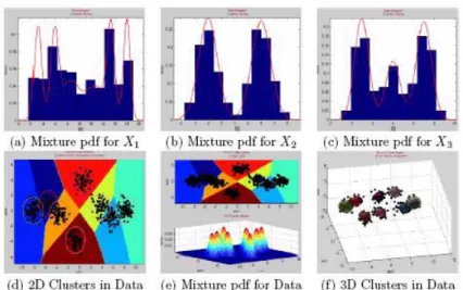
Figure 1.(Continued) The candidate component cluster centers for the bivariate normal mixture model when 1= 2 for 1and 2= 2 for 2 Let us explain the effectiveness and usefullness of the interval proposed for the on the simulated data set in Table 1. The simulated data set in Table 1 consists of three variables. 1with 6 components, 2with 2 components and 3 with 3 components. 6 ≤ ≤ 36 for the simulated data set in Table 1. The exact or true number of component clusters in the mixture model is 8, thus = 8. Graphical representations, obtained using MIXMOD, for the results of multivariate normal mixture model clustering of the simulated data set is given in Figure 2.
All traditional methods, as explained in [4], start searching for the optimal com-ponent number from 2 in the algorithm. The interval in equation (4) proposes that the algorithm should start for testing the component number from 6 in the algorithm for the simulated data set considered. So testing the values 2, 3, 4, and 5 for the component number in the algorithm used in all traditional model based clustering methods is unnecessary and waste time for the simulated data set considered. The interval proposed for the for the simulated data set considered above and for the others in Table 1 seems to be a large interval as seen from the results in Table 1. But this is not important when the algo-rithm starts searching for the optimal component number from min in the model based clustering methods. The algorithm ends searching at the optimum or true component number in the model based clustering methods. For the case considered, thus the simulated data set, the proposed interval is 6 ≤ ≤ 36. The algorithm starts searching for the optimum com-ponent number from 6 (not 2) in the model based clustering methods. The algorithm ends searching for the optimum or true component number 8 (not 36).
Figure 2.Graphical representations, obtained using MIXMOD, for the results of multivariate normal mixture model clustering of simulated data set in Table1 3. The Total Number Of Candidate Mixture Models In Multivariate Normal Mixture Model Based Clustering
The interval for in equation (4) gives also extra information about the for multivariate normal mixture model clustering analysis of -dimensional multivariate data using model selection criteria. The is defined by
(5) = 2 max
where max is the maximum of the total number of candidate com-ponent cluster centers. = 2 max = 24 = 16 for the case
considered in Section 2. So the is 7 for the case considered in Section 2. Thus, bivariate normal mixture model clustering analysis of 2-dimensional multivariate data using model selection criteria. The is obtained as the sum of with 4, 3 and 2 component clusters () for the case considered in Section 2. Thus,
= 4 + 3
+ 2 (6)
Each of seven bivariate normal mixture model with 4 (Case a in Figure 1), 3 (Cases b-e in Figure 1) and 2 (Cases f and g in Figure 1) component clusters for the case considered corresponds to various clustering situations defined by Bensmail and Celeux [15] and Biernacki et al. [7] depending on the covariance matrix Σ of th component multivariate normal density of the mixture model with different characteristics [16].
The best or optimum model is chosen among these 7 possible mixture models, thus the cases (a)-(g) in Figure 1. The and the can be very important in finding the optimum or the best model. The approach, in this study, can lead a genetic algorithm for the multivariate normal mixture model clustering of multivariate data, but this is not in the scope of this study. This may be a subject of another study.
4. Some Applications Of The Interval Constructed For The Total Number Of Candidate Component Cluster Centers In Multivariate Normal Mixture Model Clustering
The interval proposed for the , in equation (4), in the multivariate normal mixture model clustering will be examined on some frequently studied data sets in the literature given in Table 1. The MIXMOD Software [7] is used in all computations, thus, in determining the number of components in each vari-able and in determining the number of component clusters in the multivariate normal mixture model for -dimensional multivariate data.
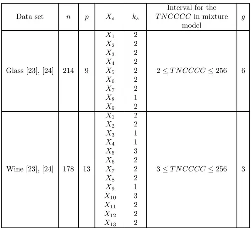
Table 1. The interval constructed for the for some frequently studied data sets ( : Number of observations or Objects, : Number of variables or Attributes, : Variables, : Number of components in each
variable, : Exact number of component clusters in mixture model).
Data set
Interval for the in mixture model Geyser [17] 272 2 1 2 3 2 3 ≤ ≤ 6 3 Ruspini [18], [19] 75 2 1 2 2 4 4 ≤ ≤ 8 4 Diabetes [20], [21] 145 3 1 2 3 2 3 2 3 ≤ ≤ 12 3
Simulated Data Set 600 3 1 2 3 6 2 3 6 ≤ ≤ 36 8 Iris [16], [19], [22] 150 4 1 2 3 4 2 1 3 3 3 ≤ ≤ 18 3
Table 1(continued). The interval constructed for the for some frequently studied data sets ( : Number of observations or Objects, : Number of variables or Attributes, : Variables, : Number of components
in each variable, : Exact number of component clusters in mixture model)
Data set
Interval for the in mixture model Artificial Data set 1 [6] 300 4 1 2 3 4 3 3 2 2 3 ≤ ≤ 36 7 Liver Disorders [23] 345 6 1 2 3 4 5 6 1 2 2 2 2 2 2 ≤ ≤ 32 2 Pima Indian Diabetes [24] 768 8 1 2 3 4 5 6 7 8 2 2 1 2 2 1 2 2 2 ≤ ≤ 64 2 Yeast [24] 1484 8 1 2 3 4 5 6 7 8 2 1 2 2 1 1 2 2 2 ≤ ≤ 32 10
Table 1 (continued). The interval constructed for the for some frequently studied data sets ( : Number of observations or Objects, : Number of variables or Attributes, : Variables, : Number of components
in each variable, : Exact number of component clusters in mixture model)
Data set
Interval for the in mixture model Glass [23], [24] 214 9 1 2 3 4 5 6 7 8 9 2 2 2 2 2 2 2 1 2 2 ≤ ≤ 256 6 Wine [23], [24] 178 13 1 2 3 4 5 6 7 8 9 10 11 12 13 2 2 1 1 3 2 2 2 1 3 2 2 2 3 ≤ ≤ 256 3
5. Discussions And Conclusions
Determining the number of component clusters is the most important problem in multivariate normal mixture model based clustering of multivariate data and determining the number of candidate mixture model is also an interesting prob-lem in multivariate normal mixture model based clustering using model selection criteria.
There are two purposes of this study. First, the total number of candidate component cluster centers is introduced and an interval is constructed by using the number of partitions in each variable in multivariate data, since the mixture structure of each variable forms the candidate component cluster centers in multivariate data. Constructing such an interval make the algorithms used in the multivariate normal mixture model clustering analysis more efficient in the
sense of operations prepared and processing time since the strategy for model based clustering takes into account the minimum and the maximum number of clusters.
All traditional methods, as explained in [4], start searching for the optimal component number from 2 in the algorithm. The interval in equation (4) pro-poses that the algorithm should start for testing the component number from min in the algorithm. For example, the algorithm should start from 6 for testing the component number in the simulated data set considered in section 2. So testing the values 2, 3, 4, and 5 for the component number in the algorithm used in all traditional model based clustering methods is unnecessary and waste time in the simulated data set considered. The interval proposed for the for the simulated data set considered above and for the others in Table 1 seems to be a large interval as seen from the results in Table 1. But this is not important when the algorithm starts searching for the optimal component number from min in the model based clustering methods. The algo-rithm ends searching at the optimum or true component number in the model based clustering methods. For the case considered, thus the simulated data set, the proposed interval is 6 ≤ ≤ 36. The algorithm starts searching for the optimum component number from 6 (not 2) in the model based cluster-ing methods. The algorithm ends searchcluster-ing for the optimum or true component number 8 (not 36). The proposed interval for the looks in each com-ponent direction separately, since it suffers each variable from the correlation effects of others or isolates the correlation effects between the variables when the variables are not orthogonal, and then combines the componentwise results to obtain the final interval. It works well also with overlapping clusters or clusters with different shapes. It is easy to detect the different centers in projections onto two dimensional plane.
Second, an equation is given for the in multivariate normal mixture model based clustering using model selection criteria. The concept is introduced. The can be very important in finding the optimum or the best model. The best or optimum model is chosen among the possible mixture models. The approach for the , in this study, can lead a genetic algorithm for the multivariate normal mixture model clustering of multivariate data, but this is not in the scope of this study. This may be a subject of another study.
Acknowledgements
We would like to thank the referees for their valuable comments and suggestions. References
1. Fraley, C. and Raftery, A. E. (2002). Model-Based Clustering, Discrimi-nant Analysis, and Density Estimation. Journal of the American Statistical Association, 97, 611-631.
2. McLachlan, G. J. and Basford, K. E. (1988). Mixture Models: Inference and Application to Clustering. New York: Marcel Dekker.
3. McLachlan, G. J. and Peel, D. (2000). Finite Mixture Models. Wiley, New York.
4. Fraley, C. and Raftery, A. E. (1998). How Many Clusters? Which Clustering Method? Answers via Model-Based Cluster Analysis. The Computer Journal, 41, 578-588.
5. McLachlan, G. J. and Chang, S. U. (2004). Mixture Modeling for Cluster Analysis. Statistical Methods in Medical Research 13, 347-361.
6. Galimberti, G. and Soffritti, G. (2007). Model-based methods to identify multiple cluster structures in a data set. Computational Statistics and Data Analysis. doi 10.1016/j.csda.2007.02.019.
7. Biernacki, C., Celeux, G., Govaert, G. and Langrognet, F. (2006). Model-based cluster analysis and discriminant analysis with the MIXMOD software. Computational Statistics and Data Analysis, 51, 587-600.
8. McLachlan, G. J. and Krishnan, T. (1997). The EM Algorithm and Exten-sions. New York, Wiley.
9. Celeux, G. and Diebolt, J. (1985). The SEM algorithm: a probabilistic teacher algorithm derived from the EM algorithm for the mixture problem. Comp. Statis. Quaterly, 2, 73-82.
10. Celeux, G. and Govaert, G. (1992). A Classification EM Algorithm for Clustering and Two Stochastic versions. Computational Statistics and Data Analysis, 14, 315-332.
11. Akaike, H. (1974). A new look at the statistical model identification. IEEE Transactions on Automatic Control 19 (6): 716—723.
12. Schwarz, G. (1978). Estimating the dimension of a model, Ann. Statist. 6 pp. 461—464.
13. Bozdogan, H. (1994). Mixture-Model Cluster Analysis Using Model Selec-tion Criteria and a New InformaSelec-tion Measure of Complexity. In Proceedings of the fist US/Japan Conference on the Frontiers of Statistical Modeling: An Informational Approach, ed. Bozdogan, Vol. 2, Boston: Kluwer Academic Publishers, pp. 69-113.
14. Soffritti, G. (2003). Identifying multiple cluster structures in a data matrix. Communications in Statistics, Simulation & Computation, Vol. 32, Issue 4, pp. 1151-1181.
15. Bensmail, H. and Celeux, G. (1996). Regularized Gaussian Discriminant Analysis Through Eigenvalue Decomposition. Journal of The American Statis-tical Association, 91(436), 1743-8.
16. Biernacki, C., Celeux, G., Govaert, G. and Langrognet, F. (2005). Model-based cluster analysis and discriminant analysis with the MIXMOD software. INRIA Institute National de Recherche en Informatique et en Automatique. No:0302, January 2005, Rapport Technique.
17. Venables, W. N. and Ripley, B. D. (1994). Modern Applied Statistics with S-Plus. Springer, 462 pages, ISBN 0 387 94350 1.
18. Kaufman, L. and Rousseeuw, P. (1990). Finding Groups in Data: An Introduction to Cluster Analysis. New York: Wiley-Interscience.
19. Sandra, C. M. and Leandro, N. De C. (2006). Data clustering with particle swarms. IEEE Congress on Evolutionary Computations. Sheraton Vancouver Wall Center Hotel, Vancouver, BC, Canada. July 16-21, 2006.
20. Symons, M. J. (1981). Clustering criteria and multivariate normal mixtures. Biometrics, 37, 35-43.
21. Banfield, J. D. and Raftery, A. E. (1993). Model-based Gaussian and non-Gaussian clustering. Biometrics. 49, 803-821.
22. Scott, A. J. and Symons, M. J. (1971). Clustering methods based on likelihood ratio criteria. Biometrics. 27, 387-397.
23. Halbe, Z. and Aladjem, M. (2005). Model-based mixture discriminant analysis — an experimental study. Pattern Recognition. 38, 437-440.
24. Newman, D. J., Hettich, S., Blake, C. L. and Merz, C. J. (1998). UCI
Repos-itory of machine learning databases [http://www.ics.uci.edu/ ~mlearn/MLReposRepos-itory.html]. Irvine, CA: University of California, Department of Information and Computer
Science.Golub, G. H., Heath, C. G., and Wahba, W. (1979). Generalized cross-validation as a method for choosing a good ridge parameter. Technometrics, 21, 215-223.