Optimal control for hybrid system

YASAR UNIVERSITY

GRADUATE SCHOOL OF NATURAL AND APPLIED SCIENCE

OPTIMAL CONTROL FOR HYBRID SYSTEM

İpek Yeşim CINGILLIOĞLU

Thesis Advisor: Assist. Prof. Dr. Shahlar MEHERREM

Department of Mathematics

Bornova-İZMİR 2012

ABSTRACT

OPTIMAL CONTROL FOR HYBRID SYSTEM

CINGILLIOĞLU, İpek Yeşim Master Thesis in Mathematics

Supervisor: Assist. Prof. Dr. Shahlar MEHERREM May, 2012

This thesis includes a different approach for solving optimal control for switched systems. We focus on problems in which a prespecified sequence of active subsystem is given. For these problems we must have optimal switching instants and optimal

continuous inputs. For this reason the derivatives of optimal cost with respect the switching instants need to be known.

Also in thesis an approach for solving optimal control problems of switched system.In general,in such problems one needs to find optimal continuous inputs and optimal switching sequences. After formulating a general optimal control problem, we study two stage methodology. Since many practical problems only concern optimization where the number of switchings and the sequence of active subsystems are given, we think about on such problems and propose a method which uses nonlinear optimization and is based on direct differantiations of value functions.

It is also developed a computational method for solving an optimal control problem which is governed by a switched dynamical system with time delay. Our approach is to parametrize the switching instants as a new parameter vector to be optimized. Then,we derive the required the gradient of the cost function which is obtained via solving a number of delay differential equations forward in time. Finally, there are given optimality condition for the switching control system.

Keywords: Switched system, Delay, Parametrization, Optimal control.

Yüksek Lisans tezi olarak sunduğum ‘’Hybrid System for Optimal Control’’ adlı çalışmanın, tarafımdan bilimsel ahlak ve geleneklere aykırı düşecek bir yardıma

başvurmaksızın yazıldığının ve yararlandığım eserlerin ‘’Bibliography’’ bölümünde gösterilenlerden oluştuğunu, bunlara atıf yapılarak yararlanılmış olduğunu belirtir ve bunu onurumla doğrularım.

…./…./20

İpek Yeşim CINGILLIOĞLU

TEŞEKKÜR

Yüksek lisans tezimi hazırlarken bana rehberlik eden ve desteğini eksik etmeyen danışman hocam Yrd. Doç. Dr. Shahlar MEHERREM’e , lisans ve yüksek lisans eğitimimde ders aldığım tüm hocalarıma, hazırlık aşamasında yardımcı olan tüm sevdiklerime teşekkür ederim.

İpek Yeşim CINGILLIOĞLU

1. NECESSARY OPTIMALITY CONDITIONS FOR SWITCHED SYSTEM

1.1 Switching Systems

1.2 Approach Based on Parametrızation of the Switching Instants 2. SWITCHED OPTIMAL CONTROL FOR

NONLINEAR OPTIMIZATION PROBLEM

2.1 Switching Systems 2.2 Two or More Switching

3. TIME DELAY OPTIMAL CONTROL PROBLEM

3.1 Problem Formulation 3.2 Problem Reformulatıon and Gradient Formula

3.3 New Results and Open Problems and Problem Formulation CONCLUSION

BIBLIOGRAPHY

INTRODUCTION

Switched system are class of hybrid systems which consists of several subsystems and switching law orchestrating the active subsystemat each time instant.

Optimal control problems for switched systems ,which require the solutions of both the optimal switching sequences and the optimal continuous input. Many results,which report progress regarding the theoretical or practical issues for continuos time or discrete time versions of such problems, appeared the literature [1],[5],[6]

Maximum principle and Hamiltonian Jacobi-Bellman equation for hybrid and switched systems derived in literature [4].Optimal control problems of hybrid and switched systems have been attracting researches from various in science and engineering significance in theory and application,classifiedto categories, theoretical and practical. These results extended classical maximum principle or dynamic programming approach for problems. Also, proves a maximum principle for hybrid system with autonoumus switching only. Another result is proof of existence of optimal control for system with two subsystems. Complicated versions of maximum principle under additional

assumptions.

The problem formulations and methodologiesare very diverse in this category It is important that in thesis have different models and optimal control objarctives for hybrid system. This thesis presents solving optimal control problems of switched systems. This thesis presents solving of optimal control problems for switched systems. In thesis focused on problem which a presrecified sequence of active subsystems is given. From here, in thesis, need to seek optimal instants ans optimal continuous inputs. In order to redsearch for optimal switching instants,the derivatives of the optimal cost need to be known. It is important that, method is trancribes an optimal control problem into an equivalent parametrized by the switching instants and derives the derivatives based on solution of a two boundary value formed by state, costate, stationary equations, the boundary and continuity conditions with their differentiations.

In the thesis our approach is to parametrize the switching instants a new parameter vector to be optimized. After,derived gradient of cost function which is obtained via solving a number of delay differential equations in time.

1.1 Switched Systems

We think about switched systems consisting of the subsystems

̇ = { } (1.1.1) From control switched system we must have continuous input and switching sequence.

A switching sequence in t [ , ]t t_{0 f} regulates the sequence of active subsystems and is

defined as ( ) where , _and (1.1.2) for k= .

Note that, indicates that at instant t_k the system switches from

subsystem during the time interval [ ] ([ ) subsystem k

i is active. For switched systems we consider nonZeno sequences which switch at most finite number of times in [ ] Also we regard  which discrete input, then we have control input u with .

Finally, switching system from general hybrid system is continuous state and does not jumps at switching instants.

Optimal control problem

In the sequel, _{[ ]} , which means that { [ ] } We concentrate on problems which involve optimizations and prespecified sequence of active subsystems.

Problem 1: Think about switched systems which consists of subsystems ̇

Given a fixed time interval [ ] and a prespecified sequence of active subsystems , find a continuous input _{[ ]}and a switching

instants such that the corresponding continuous state trajectory x departs from a given initial state

{ }

and the cost functional

( ( )) ∫ (1.1.3) is minimized.

In order to solve problem 1, needs to also nonlinear optimization techniques.

Problem 1 is basic optimal control of Bolza form. In the sequel, we assume that

are continuous and have continuous partial derivatives with respect the ; f is

1 with a fixed final time is mainly fort he convenience of subsequent studies. For with free final time , we can introduce an additional state variable and transcribe to fixed final time problem.

Two stage decomposition

Stage (a) is conventional optimal control problem which is research the minimum value of with respect the u under given switching sequence

( ) In the sequel,we define the coresponding optimal cost function ̂ , ̂ { }

Stage (b) is constrained nonlinear optimization problem ̂ , ̂

(1.1.4) { ̂ } In order to solve Problem 1, we need

nonlinear optimization techniques.

Stage(a): We need to find an optimal continuos input u and minimum . Although

different subsystems are active in different time intervals, stage(a) research ̂ for ̂ is conventional intevals are fixed.

Theorem 1: Necessary conditions for stage (a): Think about the stage (a) problem for problem

1. Assume that subsystem k is active in [t_k1, )t_k for 1 k K and subsystem K1 in [ ] with Let _{[ ]} be a continuous input such that the

coresponding continuous state trajectory departs from given

and { } In order for u to be optimal it is necessary that vector function [ ] [ ] such that following conditions hold;

a) For almost any [ ] the following state and costate equations hold: state equation: ( )

(1.1.5) costate equation: ( ( ))

(1.1.6) Here [ if if [ ].

( ( ))

c) At ( ) ( ( )) ( ( )) (1.1.8)

where is an dimensional vector.

d) At any _{, we have}

(1.1.9) Proof: Using Lagrange multipliers to adjoin the constraints

̇ and ( ) to The augmented performance index is

( ) ( ) ∑ ∫( ̇ )

by

[ , and [ ] with

if k K 1 ( ( )) ( ( ))+ ∑ (

̇) , from calculus of variations ( ( ( ))

( ( )) ( )) ( ) ∑

∑ ∫ (( ̇ ) )

( ̇ )

From Lagrange theory a necessary condition for a solution to be optimal is =0. Setting the zero the coefficients of the independent increments ( ) _{yields the necessary conditions a)-d).}

The conditions a)-d) present a two boundary value differential algebraic equation (DAE), which solved numerical methods.

Stage(b): We need to solve the constrained nonlinear optimization problem( 4) with simple constraints. Computational methods for finding local optimal solutions of such problems are abundant in nonlinear optimization literature.

1.2 Approach Based on Parametrization of Switching Instants

In thesis an approach to problem 1 based on parametrization of the switching instants is presented. The first step is transcribe an optimal control problem into an equivalent conventional optimal control problem parametrized by the switching instants.

Equivalent problem formulation

Here, defined the transcription of problem 1 into an qeuivalent problem

parametrized by the unknown switching instants also switching instants are fixed with respect to new independent time variable. We think about two subsystems where

subsystem 1 is active in [ and subsystem 2 is active in [ ] and also

Problem 2: For switched system ̇ = (1.2.1) ̇ = (1.2.2)

Find a switching instant and a continuos input , [ ] suh that

( ) ∫ (1.2.3) is minimized.

For transcribe equivalent problem 2 we define a state variable coresponding switchinginstant

Let satisfy (1.2.4) (1.2.5) Next, we introduce . A piecewise linear relation ship between t and is

0 ( n 1 0)

t t x _ t 0  1 and {( ( ) )} for

(1.2.6) By introducing and, problem 2 is transcribe into following problem.

Problem 3 (Equivalent problem) : For system with dynamics

(1.2.7) and for [ (1.2.8) and (1.2.9) (1.2.10)

in[1, 2], find and [ ] such that;

∫ ∫ ∫

(1.2.11) Note that problem 2 and problem 3 are equivalemt in optimal solution for

problem 3 is an optimal solution for problem 2 by proper change of independent variable and by regarding

Method based on solving a boundary value differential algebraic equation

We develop a method for deriving accurate numerical value . The method is based on the solution of a two boundary value DAE formed by state, costate, stationary equations, the boundary and continuity conditions for problem 3, along with their derivatives with respect to parameter

Think about the equivalent Problem 3, define

̃ (1.2.12) ̃ (1.2.13)

̃ (1.2.14) ̃ (1.2.15)

Consequently we denote it as . We define the parametrized

Hamiltonian as 1 ( , , , _n ) H x p u x _ { ( , ,L x u x_{1 n1}) p f x u xT ₁( , , _{n 1})      [0,1) 1 ( , , , _n ) H x p u x_ { ( , ,L x u x₂ n ₁) p f x u xT ₂( , , n₁)      [1, 2] (1.2.16) The necessary conditions a) and b) provide us with following state, costate, stationary equations: ( ) ̃ (1.2.17) ( ) ( ̃ ) ( ̃ ) ( ) ( ̃ ) ( ̃ ) (1.2.19)

Note that pand u are coresponding to optimal solution are also functions of  and .

From the necessary condition c) of theorem 1, we have

(1.2.20) ( ) (1.2.21) the necessary condition d) tell us is continuous at for fixed

(1.2.22)

Then we have optimal value of J which is function of the parameter

( ) ∫ ̃ ∫ ̃ (1.2.23) ( ) ∫ ( ( ) ( )) ∫ ( ( ) ( )) (1.2.24) .

So must have and

( is fixed) in order to the value

Then; ( ) ( ) ( ) (1.2.25) ( ) ( ) ( ) ( ) (( ) ( ) ( ) ) (1.2.26) ( ) ( ) ((₍ ) ( ) )) (1.2.27) for [ and ( ) ( ) ( ) ( ) (1.2.28)

( ) ( ) ( ) ( ) ( ) (( ) ( ) ( ) ) (1.2.29) ( ) ( ) ( ) ( ) ( ) ( ) (1.2.30) For [ ]

Differentiating the boundary conditions (1.2.29) and (1.2.30) and the continuity condition (1.2.31) with respect to , obtain that,

(1.2.32) Problems with internally forced switchings

The specifications of switched system with IFS included the switching sets where . In thesis

{ }.

Here we focus on optimal control roblems for switched systems withIFS in which a prespecified sequence of active subsystem is given.

Problem 4: Consider system with IFS. Given fixed time interval [ , ]t t_{0 f} and

prespecified sequence of active subsystem, find continuous input _{[ ]}such that the coresponding continuos state trajectory departs from a given initial state and

{ } (( )) ∫ ( ) is minimized.

Problems of internally forced switching Approach 1

1) Denote in redundant fashion that an optimal solution to an ıfs problem contaşns both optimal switching sequence and an potimal continuous input,i.e, regard an ıfs problem as an efs(externally forced switching) instants.

2) Verify the validitynof solution fort he ıfs problem if the system under the continuous input can evolve validly and generate the coresponding switching sequence.)

Theorem 2: Consider stage(a) for problem (4). Assume that subsystem k is active in

[

for 1 k Kand subsystem K1 in [ ) = Assume that { } at t . Let k [ ] such that the coresponding

continuos state trajectory departs from a given initial state and { }

Also assume that for t(t_k1, )t_k 1 k K and for

t( , )t_K t_f . In order to u be optimal,it is necessary that there exist vector function [ [ ] such that conditions a)-c) as in theorem 1 hold, the condition hold.

d) At any ,k =1,2,…,K,we have +(( ) ) .

Proof: Similar to theorem 1,except that here in , we introduce a term ( )

and in ,we have coefficients of as +(( ) ) Setting to zero coefficients of the independent increments of ( ) therefore yields the necessary conditions a)-d).

2. SWITCHED OPTIMAL CONTROL FOR NONLINEAR

OPTIMIZATION PROBLEM

2.1 Switched Systems

Definition:

is directed graph indicating the discrete structure of system. The node set { } is the set of indices for subsytems . The directed edge set E is a subset of { } which contains all valid events.If an event takes place,the system switches from subsystem i to₁ i . { ₂ } with describing the vector field for the subsystem ̇ ,then the switched system can be define as,

̇ (2.1.1)

(2.1.2) where determines the active subsystem at instant t.

Definition: For switched system a switching sequence  in [ , ]t t_{0 f} is defined as ( ) (2.1.3)

with for . We define _{[ ]} in[ ].

An optimal control problem

Problem 2.1 Consider a switched system S=(D,F).Given a fixed time interval[ ], find a picewise continuous input u and switching sequence such that is minimized ∫ L t tf

t (2.1.4)

Here

Problem 2.1 is basic optimal control problem in Bolza form. we assume that f,L are continuous and have continuous partial derivatives with respect the _{is continuos} derivatives.

Two stage optimization

We need to find optimal control solution for Problem 2.1 such that

Note that for any fixed , Problem 2.1 reduces to conventional optimal problem which we need to find that minimizes = . For this reason,

Lemma: For problem 2.1 if

a) an optimal solution exist and

b) for any fixed , there exist a corresponding * *

u u_ such that J( , ) u is minimized, then following equation holds,

[ ] [ ] [ ] [ ] (2.1.6)

Proof: Firstly,

[ ] [ ] [ ] [ ]

(2.1.7) Because for any fixed ,there exist *

u_ such that

[ ] .But for every pair ( we must have , therefore from (2.1.7) we must have

[ ] [ ] [ ] (2.1.8) While we have inequality,

[ ] [ ] [ ] ) (2.1.9) we can choose since for any other u ,we must have , due to the

optimality of , . Hence combining (2.1.8) and (2.1.9) we have _{[ ]}

[ ] (2.1.10) Hence all inequalities in (2.1.10) must be inequalities and the

[ ] can be replaced by _{[ ]}, so we obtain that

[ ] [ _] [ ] _{[ ]} (2.1.11)

Two stage optimization problem

Stage 1 . Fixing ,solve the inner minimization problem. Stage 2. Regarding the optimal cost for each as a function.

(

[ ] (2.1.12) Minimize with respect to _{[ ]}

Algorithm (A Two Stage Algorithm)

Stage 1 a) Fix the total numbwer of switchings to be K and the sequence of active subsystems and let the minimum value of with respect to be i.e, function of the K switching instants for ( ) for K Find _{b) Minimize it.}

Stage 2 (a) Vary the sequence of active subsystems to find an optimal solution under switchings.

(b) Vary the number of switchings to find an optimal solution for problem 2.1.

More on stage 1 optimization

We concentrate of on stage 1 optimization. Stage 1(a) is in essence a conventional optimal control problem which seeks the minimum value of J with respect to u under given switching sequence ( )

Stage 1(b) is in esence a constrained nonlinear optimization problem,

_{̂ ̂ subject to (2.1.13)} where { ̂ } In order to stage 1 problem,one

needs to resort to not only optimal control methods, also nonlinear optimization techniques.

Stage 1(a)

For stage 1(a) where switching sequence ( ) is given , finding ̂ for the coresponding ̂ is a conventional optimal control problem. We need to find an optimal continuos input u and the coresponding . In order to find solutions for stage 1(a) problems,computational methods must be adopted in most cases. Most of available numerical methods are for unconstrained conventional optimal control problems with fixed end time can be used.

Stage 1(b)

We need to solve the constrained nonlinear optimization problem (4.1) with simple constraints. Computational methods for the solution of such problems are abundant in the nonlinear optimization literature.

Algorithm (A conceptual Algorithm For Stage 1 Optimization) (1) Set the iteration index . Choose an initial ̂

(2) By solving an optimal control problem stage1 (a), find ( ̂ ) (3) Find _̂ and _̂ ̂ .

(4) Use some feasible direction method to update ̂ to be ̂ _{̂ ̂ . Set the}

iteration index .

(5) Repeat steps (2),(3),(4) and (5), until prespecified termination condition is satisfied. Key elements of the above the algorithm are

(a) An optimal control for Step (2).

(b) The derivations of _̂ and _̂ ̂ for step (3). (c) A nonlinear optimization step algorithm for step (4).

Optimization for stage 1 problem based on direct differentiations

We propose a method to approximate the values of _{̂ ̂} ( ̂ ) and which can be used in stage1(b)optimizations. The method is based on direct differentiations of the value functions. We have assume that u is piecewise differentiable. We need to find an optimal switching instant vector ̂ and optimal control inputu .

Assume that we have nominal ̂ and nominal control input u which is piecewise smooth. If they are both fixed,then the cost J will be function of , but if u is fixed and ̂can be varied in small neighborhood of nominal value,then cost will be function of

Now let us assume that along with the small variations of ̂,u varies correspondingly in the following manner. If varies to ̂ ̂, u varies correspondingly to

t ̇ _{, if [ for}

t ̇ _{, if [ ] for}

Where ̇

and ̇

. We say that u assumes open loop variations in

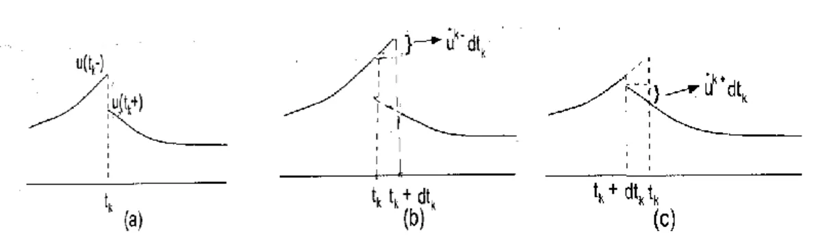
this case means that u t( ) only has variations in the interval between and as shown in figure 1. We denote such a cost value function(which is not necessarily optimal)

( ( )) ∫ ∫ _(2.1.15) where the superscript 0 is to indicate that the starting time for evaluation is We can

define the value of function at the th switching instant as

( ( )) ∫ ∫

(2.1.16)

Figure 1: The solid curves are . (a) The nominal input . (b) The open loop

variations of u t( ) induced by (c) The open loop variations of induced by

Single switching

Assume that we are given nominal , a nominal u and the coresponding nominal state trajectory . We denote ̂ and ̂ t)o be input and state trajectory after variation has taken place. We can write function with a superscript 1-(resp 1+) whenever it is evaluated at and the nominal values

resp. and the nominal values . Examples of this notational convention are

It is not diffucult to see that ∫ (2.1.17)

For a small variation of , we have

̂ ∫ (2.1.18)

The first term in (2.1.18) can be expanded into second order as

̂ _(2.1.19) where ̂ _̇ (2.1.20) The second order expansion of the second term is derived as follows by distinguishing the

case of If , we have ∫ ̂ ̂,t ∫ ∫ ∫ _(2.1.21) ıf ,we have ∫ ̂ ̂, ∫ ∫ = ∫ (2.1.22)

which has same expression as (2.1.21) for dt₁0 although the derivation is slightly different. Note that ,

̂( ) ̇ for

̇ fordt10

∫ _(2.1.24) = ( ) [ ̇ ̇ ] (2.1.25)

Consider is value function for given nominal value u t( ).

We have (2.1.26) By differentiating (2.1.25) , we obtain ̇ _{̇ (2.1.27)} By substuting (2.1.25), (2.1.26), (2.1.27) we can write

_{(2.1.28) ( ) ( ) ̇ ̇} (2.1.29) 2.2 Two or more switching

From second order optimization algorithm ,for switched system two or more

switchings,we neeed more information to derives of with respect to t_k’s. Let us first consider case of two switchings. Assume that a system switches from subsystem 1 to 2 at t and from subsystem 2 to 3 ₁ . The value function is then,

. The value function is then,

∫ (2.2.1)

∫ (2.2.2)

Definition (Incremental change) : Given any variations and , we define

{ } { } to be incremental change of the state due to and . In detail see figure 3.

Case 1: , (see figure 3(a)).In this casex t( ) is defined to be

̂ [ ] [ ]

̂ [ ] (2.2.3)

Figure 2: The incremental changex t( ) for (a), where y t is solution of ₁( )

̇ [ ] ̂

(2.2.4)

And z t is solution of ₁( ) ̇ ̂ [ ]

Case2: dt₁0,dt₂0(see figure 3(b).)

x t( ) = ̂ [ ] [ ] z t₂( )x t t( ), [ ,t t_{2 2}dt₂] (2.2.6) 2( ) y t is solution of ̇ [ ] ̂ (2.2.7) And z t is solution of ₂( ) ̇ [ ] ̂ (2.2.8)

Case 3: dt10,dt2 0(see figure 3(c)).

x t^( )x t t( ), [ , ]t t_{1 2} ̂ [ ] ̂ [ ] (2.2.9) Wherey t3( ) is solution of ̇ ̂ [ ] (2.2.10) And z t is solution of ₃( ) ̇ ̂ [ ] (2.2.11)

Case 4: dt₁0,dt₂ 0 see figure 3(d).

x t( ) = ̂ [ ] ̂ [ ] [ ] ( 2.2.12) where is solution of ̇ ̂ [ ] (2.2.13) And z t is solution of 4( ) ̇ [ ] ̂ (2.2.14)

Note thatx t( ) defines the between and ̂ in the time interval where subsystem 2 is active.

Lemma 2.2.1: Let be areal continuous function of pair of variables ,

,u U Rm and let u t( ), a t bbe a piecewise continuos function with values inU . If  is point in(a,b) at one of the following three conditions satisfied

(a)  is a point at which u is continuous and are arbitrary real numbers, (b)  is a point at which u is continuous and are positive,

(c)  is a point at which u is continuous and are negative ,then we have

∫ (2.2.15) Here  is sufficiently small positive number and o( ) is an finite small of higher order than , i.e ⏟

=0.

Lemma 2.2.2: The expressions of and are as follows

_(2.2.16)

(2.2.17) Where A t t is transion matrix for variational time varying equation ( , )2 1

̇ (2.2.18) for y t( )t[ , ]t t_{1 2} in (2.2.18) is coresponding active subsystem vector field in [ , ]t t _{1 2} and are current nominal input and state.

The forward decoupling principle: If u assumes open loop variations ,then

(a) The value of incremental change x t( )₁ at t will not be dependent upon ₁ dt . ₂ (b) The value of incremental change x t( )₂ at t will be dependent upon ₂ dt . ₂

Lemma 2.2.3:The expression of is

(2.2.19) Proof: proof is directly from the fact that

(2.2.20) Remark: It is important that ,we delibrately express the term ,

_{explicitly because it will contribute to the coefficient}

1 2

dt dt as can be seen from the discussions below. We have expressions and we are ready to derive the coefficient for in expansion of

̂ ∫ ̂ (2.2.21) Taylor expansion of first term is

̂

(2.2.22) In (2.2.21) the terms that will possibly contribute to coefficient are those containing . They are

.

(2.2.23) Substituting into ( 2.2.22) and summing them, we have first term to the

coefficient of as [

]

(2.2.24) For the second term in (2.2.21) we have lemma.

Lemma 2.2.4: The contribution of ∫ ̂ ̂ to the coefficient ofdt dt _{1 2}

is _{. (2.2.25)}

Remark : The above this results stil holds even when .

2

2

t x

V  which can be obtained similarly to _{finally we have}

[ ] [ ] (2.2.26) This result can be extended to case of switchings to relate anddt . _k

The implementation of algorithm

This algorithm is modified version of the conceptual Algorithm 4.1 can be used for Stage 1 optimization.

Algorithm (Algorithm for stage 1 optimization) (1) Set the iteration index j0.Choose an initial ̂ .

(2) By solving an optimal control problem fort he curren ̂ t (Stage(1)a),find the coresponding optimal or suboptimal control input j

u .

(3) For the currrent ̂ and its corespondinguj,supposing that ujassumes poen loop variations, find _̂ ( ̂ ) and _̂ ( ̂ ) as approximations

to _̂ and _̂ ( ̂ )

(4) Use some faesible direction method to update to be ̂ ̂ _̂

̂ . Set the iteration index j j 1. Proof of Lemma 2.2.5: Case1: . ∫ ̂ ̂ ∫ ̂ ̂ Using lemma 2.2.1 , ∫ ̂ ̂ ̂ ̂

∫ ̂ ̂ ∫ ̂ ̂ Using lemma 2.2.1, ∫ ̂ ̂ ̂ ̂ Using lemma 2.2.1, ∫

Hence _{and we conculude that form}

property ofvariational equation that,

[ ] ̂ ∫ ̂ ̂ ∫ ̂ ∫ ̂ ̂ ∫ ̂ ̂ other terms Case 2: ∫ ∫

∫ ∫ ∫ ∫ ∫ other terms Case 3: ∫ ̂ ̂ ∫ ̇

we use last equations,

̇ ̇ And + [ ̂ ∫ ̂ ̂ ] [ ̂ ∫ ̂ ̂ ] ∫ ̂ ∫ ̂ ̂ ∫ ̂ ̂

Case 4: [ ∫ ] [ ∫ ] ∫ ] ]

Proof for Lemma 5.4: Note that

∫ ̂ ̂ ∫ ̂ { } ̂ ∫ { } ̂ ∫ ̂ ̂ ∫ _{{ }} ̂ ̂ ∫ _{{ }} ̂ ∫ ̂ ̂ ̂ ∫ ̂ ̂ ̂ Case 2: ̂ ̂ ∫ _{{ }} ̂ ̂ ∫ _{{ }} ∫ _{{ }} ∫ ∫

3. TIME DELAY OPTIMAL CONTROL PROBLEM

3.1 Problem Formulation

Consider switched dynamical systems defined in [ ] with one time delay and N-1 switches:

̇ ( ) ( ] (3.1.a) With initial condition [ (3.1.b) Where , is delay time, _{and are given}

functions. Assume that the switching sequence is preassigned, such as

(3.1.2)

where the switching times are decision variables. This approach is to find a switching vector subject to condition (2.2) for time delayed switched systems(2.1a) and (2.1b) such cost function (3.1.3) is minimized, where is solutiuon of system (3.1a) and (3.1b) at terminal time corresponding to the switching vector .

Remark

If the cost function is given by

+∫ (3.1.4) convert it into an objective function of the form (2.3) by introducing an additional state

with dynamics

̇ ( )

The objective function of (2.4) can be written as

̂( ̂ ) where ̂ [ ] and

̂( ̂ ) ( )

We assume that the following conditions are satisfied:

(1) all switching durations are larger than the delay time

(3.1.5) (2) the functions and

3.2 Problem Formulation and Gradient Formula

To solve this problem we need gradient Formula of terminal cost function with respect to switching vector

For each = - i=1,…,N (3.2.1) be duration between the switching times and .Clearly that,

∑ i=1,…,N (3.2.2) Let be duration vector.

i=1,…,N (3.2.3) ∑ (3.2.4) The determination of switching vector is equivalent to determination of duration vector.

Also, , which is dependent only on switching instants { }, can be viewed as being dependent on duration vector ,i.e,

,for ( ] Then,(2.1a),(2.1b) we can write ( ) ] (3.2.5a) With (3.2.5b) ,…, ( ) (3.2.5c) For ] and (3.2.5d) [ ] (3.2.5e) And ( ) (3.2.6) Which is solution of . .

Now this problem can be formulated as;

Given dynamical system (3.2.5) find a duration vector satisfying (3.2.3) and (3.2.4) such that the terminal cost function (3.6) is minimized.This problem referred to as problem(RP).To solve(RP),we need the gradients of terminal cost (3.6) with respsect to duration vector .Note that,

(3.2.7)

We need to able to calculate, ,

(3.2.8)

Theorem:

Let satisfy the following delay differential equations

= ( ̃ ) _̃ ( ̃ ) ̃ ( ̃ ) _̃ ( ̃ ) ̃ (3.2.9) ( ̃ ) _̃ ( ̃ ) ̃ with _(t) ( ̃ ) (3.2.10a) _{(t-h) (3.2.10b)} where ̃ _{(t-h). Then} = _. Furthermore ( ( ) ( )) (3.2.11) Where ( ) is solution of system (3.5) corresponding to duration vector

Proof: Note that are continuosly differentiable

with respect to their arguments. Thus,by taking the partial differentiation of both sides of(3.5a) with respect to , obtain

) ,…, ̃ ,…,

,…,

+ _̃ ,…, ̃ ,…, )) ̃ ,…, ,with

̃ since is dependent on those such that ∑ , it follows that

Let

New Results and Open Problems for Optimal Control Problem

3.3 Switched Systems

Definition: A switched system is a tuple where ={

} with is the vector field for the subsystem

̇ { } is the set of indices of subsystems

D= is a simple finite state machine which can viewed as directed graph. I serves as the set of discrete states indexing the subsystems. { } is a collection of events. If an event takes place, the switched system will switvh from subsystem to

Aswitched system is a collection of subsystems which are related by a switching logic restricted by

The continuous state and contnuous input satisfy and . Then switched system can be described as

̇ = (3.3.1) (3.3.2)

Where determines the active subsytem at time t.

Note: If = , ,then switched system is said to be autonomous.

Definition: For swiched system a switching sequence [ ] is defined as

( ) (3.3.3) With and

for and is active in [ if [ ] and is switched trough at instant . For switched system we consider nonZeno sequences which switch at most finite number of times in[ ] For a switched system to be well behaved ,we generally exclude undesirable Zeno phenomenon.

Note: In thesis we assume that a switching is external in the sense that it is forced by a designer.

An optimal control problem

Problem 1 For a switched system ,find a switching sequence 0

[ , ]t t_f and

an input such that cost functional ( ( )) ∫ ( ) (3.3.4) is minimized,where are given

This problem is fixed final time,free final state problem. Two stage optimization

Problem 1 requires the solution of an optimal control input such that

[ ] (3.3.5) Note that, for any given switching sequence ,Problem 1 reduces to a conventional

optimal control problem for which we only need to find an optimal continuous input as to minimize

. The following lemma provides a way to formulate (5) into a two stage optimization problem.

Lemma: For Problem 1, if

(1) an optimal solution exists and

(2) for any given switching sequence ,there exists a corresponding such that is minimized,then following euations hold

[ ] [ ] (3.3.6 ) Two stage optimization method

Stage 1 Fixing ,solve the iner minimization method.

Stage 2 Regarding the optimal cost for each as a function minimize with respect to

0 [ , ]t t_f .

This method is difficult to handle.From here the above method is using. Algorithm

1 . Fix the total number of switching s to be and the order of active subsystems,let the minimum value of with respect to be a function of the switching instants,i.e,

for and then find . 2. (a) Minimize with respect to

(b) Vary the order of active subsystems to find an optimal solution under switchings.

(c) Vary the number of switchings to find an optimal solution for problem 1. Note : This algorithm has high computational costs.In practice we usually find suboptimal solutions with fixed number of switchings by using steps 1,2(a),2(b). The variational approach to optimal control problems

We derive necessary conditions for optimal control assuming that the admissible controls are not bounded.

Necessary conditions for optimal control The problem is to find an admissible control which causes the system

̇ (3.3.7) To follow an admissible trajectory minimizes the performance measure

( ) ∫ (3.3.8) admissible state and control regions are not bounded also , are specified.

Usually is state vector and is vector of control inputs. The control inputs are independent functions.

Assume that is differentiable function , then,

( ( ) ) ∫ [ ] (3.3.9) so performance measure can be expressed as

∫ { [ ]} (3.3.10) and are fixed and minimization does not affect the , so we think

about only

∫ { [ ]} (3.3.11) Using chain rule of differentiation,

∫ { [ ] ̇ } (3.3.12)

From differential equation constraints,we form augmented functional

∫ { [ ] ̇ [ ̇ ] } (3.3.13) is lagrange multipliers. ̇ [ ̇ ] [ ] ̇ so that ∫ { ̇ } (3.3.14) Assume that can be specified or free. To determine we define

̇ so [ ̇ ( ( ) ̇ ( ) ( ) ( ) )] [ ( ) ̇ ( ) ( ) ( ) [ _̇ ( ( ) ̇ ( ) ( ) ( ) )] ̇ ( ) ] ∫ {[[ _̇ ( ( ) ̇ ( ) ( ) ( ) )] [ _̇ ( ( ) ̇ ( ) ( ) ( ) )] ] [ ( ( ) ̇ ( ) ( ) ( ) )] [ _̇ ( ( ) ̇ ( ) ( ) ( ) )] } (3.3.15) Notice that ̇ and ̇ do not appear.

[[ ] ̇ ] { _̇[[ ] ̇ ]}

(3.3.16) Writing out the indicated partial derivatives gives us

[ ] ̇ [ ] [ ] (3.3.17) With applying chain rule

[

ıf assume that second order partial derivatives are continus,the order of differentiation

can be interchanged ,and these terms add to zero.In the integral term , ∫ {[[ ] _[ ] [ _]] [[ ] _[ ]] [[ ̇ ] ] } (3.3.18) This integral must vanish on extremal regardless of the boundary conditions. First observe that

̇ (3.3.19a) must be satisfied by an extremal so that coefficient of is zero. Lagrange

multipliers are arbitrary so is zero that is ̇ _[

]

(3.3.19b)

. is independent so its coefficient must be zero

[ ] (3.19c) The variation must be zero so

[ ( ) ] [ ( ( ) ( ) ) ( ) _{[ ( ( ) ( ) )]]} (3.3.20) . It is important that these necessary conditions consist of a set of ,first order

differential equations . The solution of the state and costate equations will contain constants of integration. To evaluate these constants using equations and additional set of or relationships depending on whether or not is specified from equation (15). In the following find it convenient to use the function called Hamiltonian ,defined as

[ ] (3.3.21) We can write necessary conditions:

̇ ̇ for all [ ]. (3.3.22) And [ ( ( ) ) ( )] [ ( ) ( ) ( ) ( ( ) )]

CONCLUSION

In thesis, reults for optimal control for hybrid system are reported. We studied optimal control problems for switched systems in which prespecified sequence of active subsystem is given. Idea of two stage optimization , proposed method to obtain accurate values of derivatives that is necessary for stage (b). This method is trancribes an optimal control problem into an equivalent parametrized by the switching instants and derives the derivatives based on solution of a two boundary value formed by state, costate, stationary equations, the boundary and and continuity conditions.

Then, we considered class of optimal control problems governed by switched systems with time delay. We parametrized switching instants and derived the required gradient of cost function, which some delay differential equations are required to be solved forward in time.

BIBLIOGRAPHY

1 A. Bemporad,F.Borrelli,M.Morari, ‘’Optimal controllers for hybrid systems statibility and piecewise linear e plicit form,’’ in Proc. 9th IEEE Conf Decision Control,2000, pp. 1810-1815.

2 B.Piccoli, ‘’Hybrid systems and optimal control’’,in Proc. 7th IEEE Conf. Decision Control,1998, pp. 13-18.

3 F.L.Lewis, Optimal control. Newyork : Wiley 1986.

4 H.J.Sussman ‘’ A ma imum principle for hybrid optimal control problems,’’ in Proc. 38th IEEE Conf. Decision Control,1999, pp, 425-430.

5 H.S. Witsenhausen, ‘’A class of hybrid state continuous-time dynamic systems, ‘’ IEEE Trans. Automat. Contr, vol, AC-11, pp, 161-167, Apr.1966.

6 J. Lu, L. Liao, A. Nerode, J.H.Taylor ‘’Optimal control systems with continuous anddiscrete states,’’ in Proc. 2nd IEEE Conf. Decision Control,1993, pp. 2292-2297. 7 J. Young, ‘’Systems governed byordinary differential equations with continuous, switching and impulse controls.’’ App.Math.Optim,vol,2 , pp, 22 -225,1989 8 K.Gokbayrak and C.G Cassandras, ‘’Hybrid controllers for hierarchically

decomposed systems’’,in Proc.Hybrid systems Computation Control, vol.1790,2000, pp. 117-129.

9 M. Athans and P.Falb,Optimal Control. Newyork: McGraw-Hill, 1966

10 M.S.Branicky,V.S.Borkar,S.K.Mitter, ‘’Aunified framework for hybrid control model and optimal control theory’’, IEEE Trans. Automat. Contr, vol 4 , pp. 1-45,1998.

11 Sh. Maharromov, ‘’Necessary Optimality for Switching Optimal Control Problem’’ American Institue of Mathematics, Journal of Industrial and Management

Optimization (SCI), 47-56 pp, 2010

12 Sh. Maharromov, ‘’Optimality Condition for Nonsmooth Switching Control Problem’’Authomatic Control and Computer Science,94-101pp,2008

13 Sh. Maharromov and K.Msnsimov, ‘’Optimization of Class of Discrete step control System’’, Journal of Computational mathematics and Mathematical Physics (Russian academy of Science), 360-366pp,2001.

14 Sh. Meherrem and R.Polat,Weak subdifferential in Nonsmooth Analysis and Optimization, Journal of APPLİED Mathematics SCI , 2 11 p.1-9

15 S. Hedlund and A.RANTZER , ‘’Optimal control of hybrid system’’ in Proc. 8 th IEEE Conf. Decision Control,1999, pp. 1972-3977.

16 T.I.Seidman ‘’Optimalcontrol for switching systems, in Proc. 21st Annu. Conf. Information Sciences Systems,1987, pp, 485-489.

17 X. Xu, P. J. Antsaklis, ‘’Optimal control of switched systems New rsults and open problems,’’ in Proc,2 ,Amer, Control Conf, 2 , pp, 268 -2687.

18 X. Xu ‘’Optimal control of switched systemsvia nonlinear optimization based on direct differentiations of value functions,’’Int, J. Control, vol.7 , no, 16/17, pp 14 6-1426,2002.

19 P. Riedinger, C. Zanne, , Kratz, ‘’Time optimal control of hybrid systems’’, in Proc. 1999 Amer. Control Conf,1999, pp, 2466-2470.

20 T.I.Seidman ‘’Optimal control for switching systems, in Proc. 21st Annu. Conf. Information Sciences Systems,1987, pp, 485-489.