516
DOI: 10.19113/sdufenbed.677943
Optimum Laser Polishing Decision-Making for On-Demand Additive Manufacturing of
Spare Parts: An Exploratory Study
Mustafa Hekimoğlu*1 , Durul ULUTAN2
1,2Kadir Has Üniversitesi, Mühendislik ve Doğa Bilimleri Fakültesi, Endüstri Mühendisliği Bölümü, 34083, İstanbul, Türkiye
(Alınış / Received: 21.01.2020, Kabul / Accepted: 21.07.2020, Online Yayınlanma / Published Online: 20.08.2020)
Keywords
Laser polishing, Additive manufacturing, 3D printing,
Optimization
Abstract: Additive manufacturing is increasingly being used for satisfying spare
parts needs of capital products using a nearby 3D printer. Such a technology allows inventory managers to start manufacturing after the demand realization which eliminates significant portion of spare parts inventory being held due to random nature of component breakdowns. Quality difference between printed and original parts, which is one of the biggest problems of using 3D printers, can be decreased by the use of laser polishing which alleviates surface roughness and increases reliability of parts in exchange of an additional cost term. Using different parameters, reliability of parts can be altered depending on needs of capital products and systems’ status. In this study, the problem where surface roughness and reliability of printed parts are jointly optimized with inventory levels of original spare parts is considered. In the problem setting, a machine part consisting of a constant number of identical products which are subject to random breakdowns over a finite planning horizon is considered. Using mathematical analysis and exhaustive numerical experiments, the relationship between optimum control policy and cost parameters was shown, which might be critical for cost-effective management of the system.
Yedek Parçaların Talebe Yönelik Eklemeli Üretiminde Lazer Cilalamanın Optimum
Karar Verme Politikası Üzerinde Etkisi
Anahtar Kelimeler
Lazer cilalama, Eklemeli üretim, Üç boyutlu yazma, Optimizasyon
Özet: Eklemeli imalatın yakınlarda bulunan bir 3D yazıcı kullanılarak sermaye
ürünlerinin yedek parça ihtiyaçlarını karşılamak için kullanılması giderek yaygınlaşmaktadır. Böyle bir teknoloji, talebe-binaen parça üretimini mümkün kılarak arızaların rassallığı nedeniyle tutulan yedek parça envanterinin önemli bir kısmını ortadan kaldırma imkânı sunmaktadır. 3D yazıcı kullanımının en büyük sorunlarından biri olan basılı ve orijinal parçalar arasındaki kalite farkı, yüzey pürüzlülüğünü hafifleten ve ek maliyet terimi karşılığında parçaların güvenilirliğini artıran lazer parlatma kullanılarak azaltılabilir. Farklı parametreler kullanılarak, parçaların güvenilirliği, sermaye ürünlerinin ihtiyaçlarına ve sistemlerin durumuna göre değiştirilebilir. Bu çalışmada, basılı parçaların yüzey pürüzlülüğü ve güvenilirliğinin orijinal yedek parçaların envanter seviyeleri ile birlikte optimize edilmesi sorunu ele alınmıştır. Çalışmada, sınırlı bir planlama ufku üzerinde rastgele arızalara maruz kalan sabit sayıda özdeş makinadan oluşan bir üretim tesisi dikkate alınmıştır. Matematiksel analiz ve ayrıntılı sayısal deneyler kullanılarak, sistemin uygun maliyetli yönetimi için kritik olabilecek optimum kontrol politikası ve maliyet parametreleri arasındaki ilişki gösterilmiştir.
1. Introduction
Additive manufacturing (3D-printing) is a process where final product is created in a layer-by-layer
fashion [1]. Major benefits of methods of additive manufacturing compared to subtractive manufacturing methods are decreased cost in terms of lead time and setup time, decreased process
Süleyman Demirel University Journal of Natural and Applied Sciences Volume 24, Issue 2, 516-525, 2020 Süleyman Demirel Üniversitesi
Fen Bilimleri Enstitüsü Dergisi Cilt 24, Sayı 2, 516-525, 2020
517 complexity, and increased product design complexity. Despite the controversial problems additive manufacturing generated such as copyright issues, relative mobility of equipment and capability to implement the technology at low-cost has instigated considerations of innovative application ideas. One of the biggest technical issues with all additive manufacturing processes is the staircase appearance of the final product due to the layer-by-layer nature of the process [2]. In some cases where tolerances are not constraining (such as rapid prototyping), staircase appearance may not be of great importance and the product can be kept as is. However, in most modern cases, where tolerances better than those for rapid prototyping are required, staircase appearance of the product is not acceptable, therefore must be dealt with in some way. Although there are more complex methods researchers develop such as 5-axis 3D-printing and robotic 3D-printing, employing a relatively inexpensive subtractive technique to post-process the 3D-printed part to required dimensions is a favored method [3, 4]. One of these subtractive post-processing techniques is known as laser polishing, where a laser beam is focused on the part surface to eliminate irregular wavy texture that is created by the staircase appearance [5]. Therefore, the laser beam results in a smoother surface on the product than before.
Smoothness of the product surface is not merely a cosmetic issue. It is established that surface defects such as increased surface roughness result in lowered fatigue life of the end product among other worsened important mechanical properties [6]. Another major issue with 3D-printed products is their significantly lower reliability in the long run and their continuous usage. This issue is related to the reduced surface quality, which makes reducing surface roughness of 3D-printed parts a priority in the industry. Laser polishing can be utilized as an assisting subtractive process to improve surface quality and therefore the reliability of such parts [5]. However, laser polishing parameters need to be selected carefully. With incorrect sets of laser polishing parameters, a) process may not be effective in polishing the surface at all, b) process may be too slow to contribute to cost savings efficiently, or c) laser beam may burn the surface, resulting in unfavorable surface qualities as well as worsened tolerances.
With all these considered, innovative ideas of production as well as innovative ideas of process planning emerge. For example, if 3D-printers are made available more commonly in different areas of the world, different approaches to shipping and logistics can be developed. Instead of shipping finished goods from one place (e.g. warehouse) to another (e.g. plant) with special and costly packaging and care procedures, companies can ship raw materials to location and convey the design via cyber
communication. This way, many costs incurred by transportation of finished products can be eliminated. Furthermore, holding costs can be reduced significantly since inventory of finished or partially finished goods will not be necessary. Instead, companies can only store raw materials that can be used to create multiple parts whenever necessary. However, in order to facilitate all of these, companies need to have a good understanding of the processes involved in such technologies and how they can benefit from these technologies.
In this study, effect of the total cost incurred by laser polishing of 3D-printed parts on process planning is investigated. First, the theory of laser polishing of 3D-printed parts is presented in Section 2.1. Then, the mathematical model of minimizing the total discounted cost in a finite planning horizon is introduced in Section 2.2. Results of the method are presented in Section 3 with discussions and concluding remarks in Section 4.
2. Material and Method 2.1. Theory
In this work, a mathematical model that jointly optimizes inventory level and reliability of manufactured parts is presented. Inventory costs increase when multiple parts are stored as backup due to lead time and uncertain reliability considerations. In this study, additive manufacturing of backup parts is discussed, which means that inventory of significantly reduced number of different parts (raw materials) is sufficient. For example, assuming that all parts of a system can be 3D-printed with three different raw materials, total number of inventory parts can be reduced to three. Since commonality between parts is increased, total space requirement for inventory can be minimized. Therefore, with the eliminated requirement of actual part inventory, reduction of inventory costs is aimed. Reliability of spare parts also determines the viability of such a cost reduction. Reliability of parts produced, as measured with fatigue life, has been agreed to strongly depend on their surface quality. When the surface is not sufficiently smooth, cracks can initiate, propagate, and eventually lead to premature part failure due to stress concentrations on defective (non-smooth) portions. The most common method to measure surface quality is its roughness. Therefore, in order to increase reliability of additively manufactured parts, it is essential to improve the surface quality by decreasing surface roughness. The usage of post-production processes, such as laser polishing or heat treatment, increases the reliability of manufactured spare parts in exchange of increased marginal cost. Researchers considered laser polishing for reducing surface roughness of a part manufactured additively [7, 8]. They found that surface roughness of a spare part can be expressed as a convex function of the laser energy density (𝜉),
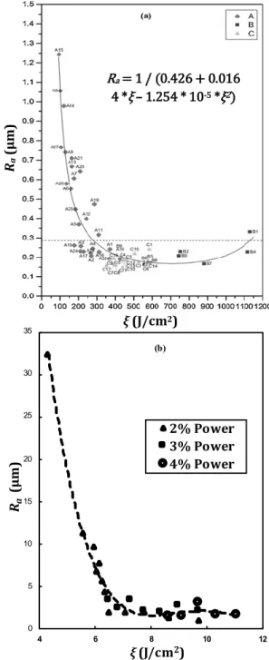
518 which is the most important factor of the laser polishing technique (Figure 1). This laser energy density (𝜉) is known to be a function of laser power P, laser speed V, and laser spot diameter D, as given in (1).
𝜉 = 𝑃
𝑉𝐷 (1)
Experimentally, surface roughness was shown to remain high at low laser energy density levels, which was attributed to the ineffectiveness of the laser beam at low power and high speed (laser beam not having an effect at all) [7]. When laser energy density is increased either by increasing laser power, decreasing speed of laser beam, or decreasing the laser spot diameter, surface roughness starts to decrease [8]. After a certain increase in laser energy density, surface roughness is observed to reach a plateau, not changing significantly with further increase in laser energy density. If the laser energy density is increased even further, it is possible that adverse effects of laser polishing (e.g. burning the surface) can outweigh its benefits. Therefore, at extremely high energy density levels, surface roughness can be expected to increase compared to the plateau reached at moderate levels. The inverse quadratic empirical model that was developed represents all of these behaviors successfully [7]. For the reader’s reference, the magnitude difference between axes of the two graphics on Figure 1 is due to the different materials used in these two studies. Chang et al. [7] suggested that there is a functional relationship between laser energy density and surface roughness. They used an inverse quadratic function where the surface roughness Ra depends only on the laser energy density 𝜉. Their resultant function is provided on Figure 1a, along with the constant values they obtained via the empirical study. In this study, a similar functional relationship is assumed between laser energy density and spare part reliability, which is directly related to the surface quality. This function is given with (2),
𝑝̃(𝜉): = 𝑝 + 1
𝑎 + 𝑟𝜉 + 𝑠𝜉2 , (2) where, constants a, r, and s are found empirically to fit the curve, with boundaries a ≥ 0, r ≥ 0, s < 0, and p is the failure probability of the original spare part within a fixed time period, such as weeks, months, etc. This mathematical model has important properties given in the following proposition:
Proposition 1: The following statements hold:
1. 𝑝̃(𝜉) is a convex function of 𝜉 and decreasing in
[0, −𝑟 2𝑠].
2. 𝑝 − min
𝜉 𝑝̃(𝜉), which is named as the originality
difference, is 4𝑠Δ, where Δ is the discriminant of
the quadratic polynomial in 𝑝̃(𝜉).
Figure 1. Experimental results and empirical
approximations of surface roughness with varying laser energy density (𝜉) by (a) [7], and (b) [8].
Proof
The first statement will be shown using the second derivative test as 𝑝̃(𝜉) is a continuous function of 𝜉. For notational simplicity, define 𝐴 = 𝑎 + 𝑟𝜉 + 𝑠𝜉2. Then 𝑝̃(𝜉) = 𝑝 +1 𝐴. 𝜕 𝑝̃(𝜉) 𝜕 𝜉 = − 𝐴′ 𝐴2 , and 𝜕2 𝑝̃(𝜉) 𝜕 𝜉2 = −𝐴′′𝐴2−2𝐴(𝐴′) 2 𝐴4 , where 𝐴 ′=𝜕 𝐴 𝜕 𝜉= 𝑟 + 2𝑠𝜉 , and 𝐴 ′′= 𝜕2 𝐴 𝜕 𝜉2 = 2𝑠. Using this, 𝜕2 𝑝̃(𝜉) 𝜕 𝜉2 = − 2 𝐴3[𝑠𝐴 − 𝐴 ′2 ] = − 2 𝐴3[𝑠𝑎 − 𝑟 2− 3𝜉𝑠𝑟 − 3𝑠2𝜉2]. This equation is positive, if 𝐽(𝜉) ≔ 𝑠𝑎 − 𝑟2− 3𝜉𝑠𝑟 − 3𝑠2𝜉2< 0, ∀𝜉 ∈ ℝ. Since 𝐽(𝜉) is a concave function, it has a single maximum point at 𝜉̅ = −𝑟
2𝑠. Substituting this value into 𝐽(𝜉), we get 𝐽(𝜉̅) = 𝑠𝑎 −𝑟42 . 𝑠 < 0 and 𝑎 ≥ 0
0 5 10 15 20 25 30 35 4 6 8 10 12 Ra (µ m ) ξ (J/cm2) 2% Power 3% Power 4% Power (b) Ra = 1 / (0.426 + 0.016 4 *ξ – 1.254 * 10-5 *ξ2) ξ (J/cm2) Ra ( µ m )
519 imply that 𝐽(𝜉) < 0, ∀𝜉 ∈ ℝ and 𝜕2 𝑝̃(𝜉)
𝜕 𝜉2 is positive as 𝐴 > 0 for 𝑥 ≥ 0. This implies that 𝑝̃(𝜉) is a convex function if the condition holds. Convexity implies that there is a unique minimizer (𝜉∗) and can be obtained with 𝜕 𝑝̃(𝜉) 𝜕 𝜉 = 𝑟+2𝑠𝜉 𝐴2 = 0 ⇒ 𝜉 ∗= − 𝑟 2𝑠. Statement 1 is proved.
For statement 2, we calculate 𝑝 − 𝑝̃(𝜉∗) for 𝜉∗= −𝑟 2𝑠. This leads us to 𝑝 − 𝑝̃(𝜉∗) = − 4𝑠2 4𝑠2 𝑎−𝑟2𝑠. Define Δ = 𝑟2− 4𝑎𝑠. Then 𝑝 − 𝑝̃(𝜉∗) = − 4𝑠2 4𝑠2 𝛼−𝑟2𝑠= 4𝑠 Δ. Q.E.D. The cost of manufacturing a part in a 3D printer, 𝑐𝑝, is considered to be lower than the acquisition cost of the original part, denoted by 𝑐𝑜. In addition, the cost of laser polishing (𝑐𝑙𝑝), which is assumed to be an additive cost component for the printing cost of spare parts, is assumed to be an increasing function of the laser energy density as follows: 𝑐𝑙𝑝(𝜉) ≔ 𝑐
0𝜉𝛾, where 𝛾 is a constant parameter depending on the polishing equipment used.
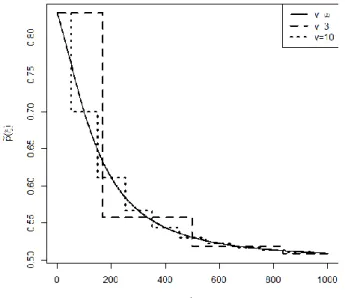
The study in this work is an exploratory one whereby developing a mathematical model that minimizes the total discounted cost that occurs in a finite planning horizon consisting of fixed time periods such as weeks, months, etc. is aimed. At each period, parts at different quality levels working in a finite amount of identical capital products, denoted by 𝑁, fail with different probabilities. For traceability of the optimal control model, we assume that there is a finite amount of different energy densities, denoted by 𝑣, that can be used in the laser polishing process. From a mathematical point of view, this is equivalent to having a finite amount of quality levels (𝑣 + 1 different failure probabilities) that can be selected for printing spare parts during the planning horizon. Two examples of such a discretization of reliability for 𝑣 = 3 and 𝑣 = 10 are given in Figure 2 against the continuous case (𝑣 = ∞).
Figure 2. Discretization of laser energy density
In the problem setting, we assume that events occur in the following order. First, delivery of the order that is placed lead time (𝑙𝑡) periods ago is delivered. After the delivery, printed parts that are working in the system, if any, are replaced with their originals. A new order, 𝑞𝑡𝑟, to the original part supplier is placed. Then random breakdowns (spare parts demand) are realized during the period. Once all random breakdowns are realized, remaining original parts are used for maintenance of those capital products. If there is no original part available, the printing process takes place. The event order of each period is depicted in Figure 3.
Figure 3. Event order within a review period
At each period of the planning horizon, a periodic cost function in (3), consisting of acquisition cost, printing cost (printing plus laser polishing), holding and downtime costs is incurred. The cost function depends on the amount of parts ordered to the original part supplier (OPS), denoted by 𝑞𝑡𝑜, parts printed at different energy densities, 𝑞̅𝑡
𝑝 ≔ (𝑞𝑡𝑝1, 𝑞
𝑡 𝑝2
, … , 𝑞𝑡𝑝𝑣), and the number of working printed parts at different quality levels denoted by 𝐦̅ .
If an original spare part is held at inventory for one period, holding cost is incurred with rate ℎ. When a capital product stays down for a period due to the lack of available (original or printed) parts, then downtime cost with a rate of 𝑏 is incurred. Assuming each machinery has a single spare part, then the conditional expectation of holding and downtime cost of a machinery can be expressed with (3).
𝐿(𝑦, 𝑞𝑝, 𝑑) = ℎ(𝑦 − 𝑑)++ 𝑏(𝑑 − 𝑦 − 𝑞𝑝)+, (3) where 𝑑̅ = (𝑑0, 𝑑1, … , 𝑑𝑣). On the right-hand-side of the equation, the first term of (3) is the amount of excess inventory at the end of a period whereas the second term is the total downtime cost at the same period given that the amount of original parts broken during a period is 𝑑0 and the number of broken parts from other quality levels are 𝑑𝑖, 𝑖 = 1,2, … , 𝑣 . Mathematical models for the optimum cost of printing and acquisition are given in (4) and (5).
520 𝑉𝑡(𝒒̅𝒕𝒓, 𝑦𝑡, 𝑚0, 𝒎̅ ) = 𝑚𝑖𝑛 𝑞𝑡𝑟≥0,{𝑐 𝑟𝑞𝑟 + ((𝑦𝑡+ 𝑞𝑡−𝑙𝑡𝑟 )⋀ ∑ 𝑚𝑖 𝑣 𝑖=1 ) 𝜓 + 𝐸 [𝐺 (𝒒̅𝒕+𝟏𝒓 , 𝑦𝑡+ 𝑞𝑡−𝑙𝑡𝑟 − ((𝑦𝑡+ 𝑞𝑡−𝑙𝑡𝑟 )⋀ ∑ 𝑚𝑖 𝑣 𝑖=1 ) , 𝑚0 + ((𝑦𝑡 + 𝑞𝑡−𝑙𝑡𝑟 )⋀ ∑ 𝑚𝑖 𝑣 𝑖=1 ) , 𝒎̿ , 𝐷𝑜, 𝐷̅𝑝)]} , (4) 𝐺𝑡(𝒒̅𝒕+𝟏𝒓 , 𝑦𝑡, 𝑚0, 𝒎̿ , 𝑑𝑜 , 𝑑̅𝑝) = 𝑚𝑖𝑛 𝑞̅𝑡𝑝≥0, (𝑑𝑜+∑ 𝑑𝑖 𝑝𝑖−𝑦)+≥∑ 𝑞 𝑡𝑝𝑖 𝑣 𝑖=1 {∑ 𝑐𝑝𝑖𝑞 𝑡 𝑝𝑖 𝑣 𝑖=1 + 𝐿 (𝑦, ∑ 𝑞𝑡 𝑝𝑖 𝑖 , 𝑑𝑜+ ∑ 𝑑𝑝𝑖 𝑖 ) + 𝛼𝑉𝑡+1(𝒒̅𝒕+𝟏𝒓 , 𝑦 − (𝑑𝑜+ ∑ 𝑑𝑝𝑖 𝑖 − ∑ 𝑞𝑡 𝑝𝑖) 𝑣 𝑖=1 , 𝑚0− (𝑑𝑜− (𝑦)+)+, 𝒎̿ − 𝑑̅𝑝+ 𝑞̅ 𝑡 𝑝 )} . (5)
The boundary condition for recursive equations (4) and (5) is 𝑉𝑇(𝐪̅𝐓𝐫, 𝑦𝑇, 𝑚0, 𝐦̅ ) = 0 for all parameters of the function.
Equation (4) gives the minimization that yields the optimum order to the OPS, 𝑞𝑡𝑟, whereas the minimization in (5) gives the optimum printing decisions, denoted by 𝑞̅𝑡𝑝
≔ (𝑞𝑡𝑝𝑖, 𝑖 = 1,2, … 𝑣) where 𝑞𝑡𝑝𝑖 is the amount of printed and polished parts using laser density level 𝜉𝑖. The reason behind optimizing these two decisions in separate minimizations is that part printing takes place after demand realization whereas, orders to OPS are placed at the beginning of a period. Therefore, the number of printed parts is a deterministic outcome of the printing policy whereas orders to OPS are placed using the expected cost. The optimum cost function 𝑉𝑡(𝐪̅𝐭𝐫, 𝑦𝑡, 𝐦̅ ) has three parameters: The first parameter is the outstanding order vector 𝐪̅𝐭𝐫: = (𝑞𝑡−𝑙𝑡𝑟 , 𝑞𝑡−𝑙𝑡+1𝑟 , … , 𝑞𝑡−1𝑟 ) including previous orders that have not been delivered. The second parameter 𝑦𝑡 is the inventory level at the beginning of period 𝑡, whereas the third parameter is the vector 𝐦̅ : = (𝑚1, 𝑚2, … 𝑚𝑣) including the amount of printed parts at quality levels 1,2, … , 𝑣.
The minimization in (4) yields the optimum order to OPS. The first term in this minimization is the acquisition cost, 𝑐𝑟𝑞
𝑡𝑟, whereas the second term represents the cost of changing printed parts upon delivery of original parts (Figure 3). The amount of
changed parts is the minimum of total available original part inventory and the amount of printed parts at work, (𝑦𝑡+ 𝑞𝑡−𝑙𝑡𝑟 )⋀ ∑𝑣𝑖=1𝑚𝑖. The total cost of changing parts before they break, which is the product of the total number of parts changed and the cost rate (𝜓), can be seen as the substitution cost of using (lower quality) printed parts instead of original part demand. The third term in the minimization gives the expected cost of printing spare parts in case of inventory shortage at the end of period 𝑡.
Given the amount of broken original and printed parts, denoted by 𝑑0 and 𝑑̅𝑝≔ (𝑑𝑝𝑖, 𝑖 = 1,2, … , 𝑣), and the vector of printed parts at work, 𝐦̿ , the summation of printing cost and the expected cost from future periods is denoted by 𝐺𝑡(𝐪̅𝐭+𝟏𝐫 , 𝑦𝑡, 𝐦̿ , 𝑑𝑜 , 𝑑̅𝑝). The first parameter of this conditional expectation is the outstanding order vector 𝐪̅𝐭+𝟏𝐫 = (𝑞𝑡−𝑙𝑡+1𝑟 , … , 𝑞𝑡−1+𝑟 , 𝑞𝑡𝑟) . Note that printing decision is made after the delivery of 𝑞𝑡−𝑙𝑡𝑟 and the placement of 𝑞𝑡𝑟 (Figure 3) so, the pipeline vector is already updated from 𝐪̅𝐭𝐫 to 𝐪̅𝐭+𝟏𝐫 . The second and the third parameters of the function are the inventory level at the beginning of period 𝑡 and the amount of original parts at work at the beginning of period t. Similarly, the amount of printed parts (at different quality levels) are denoted by the vector 𝐦̅ at the beginning of period 𝑡. Importantly, third and fourth parameters of the function Gt (.) in (5) are 𝑚0+ ((𝑦𝑡+ 𝑞𝑡−𝑙𝑡𝑟 )⋀ ∑𝑣𝑖=1𝑚𝑖) and 𝒎̿ ≔ ((𝑚1− 𝑞𝑡−𝑙𝑡𝑟 )+, (𝑚2 − (𝑞𝑡−𝑙𝑡𝑟 − 𝑚1)+)+ , … , (𝑚𝑣 − 〖(𝑞〗𝑡−𝑙𝑡𝑟 − ∑ 𝑚𝑖 𝑣−1 𝑖=1 ) + ) + ) (6)
Recall that the third parameter gives the number of original parts at the beginning of a period. After the replacement (upon delivery), the amount of printed parts is denoted by 𝐦̿ in (4). The last two parameters of the function Gt (.) are random amount of broken parts.
Total cost of printing is minimized through the vector 𝑞̅𝑡𝑝. The minimization in (5) is subject to two constraints: The first constraint is the positivity of 𝑞𝑡𝑝𝑖, 𝑖 = 1,2, … , 𝑣. The second constraint assumes that the total number of printed parts cannot be larger than the shortage of spare parts after the demand realization. This constraint is due to our assumption of preclusion of printing to stock. Under the assumption of on-demand production of spare parts with a 3D-printer that can work infinitely fast, inventory holding cost of printed parts becomes redundant.
521 The first term of the minimization gives the total cost of printing spare parts whereas the function 𝐿(𝑦, ∑ 𝑞𝑡𝑝𝑖
𝑖 , 𝑑𝑜+ ∑ 𝑑𝑖 𝑝𝑖) yields the cost of inventory holding and downtime costs. The last term, 𝑉𝑡+1(𝐪̅𝐭+𝟏𝐫 , 𝑦 − 𝑑𝑜− ∑ 𝑑𝑖 𝑝𝑖+ ∑ 𝑞𝑡 𝑝𝑖 𝑣 𝑖=1 , 𝑚0− (𝑑𝑜− (𝑦)+)+, 𝐦̅ − 𝑑̅𝑝+ 𝑞̅ 𝑡 𝑝 ), in the minimization yields the optimum discounted cost starting from period 𝑡 + 1 . In this term, the first parameter represents the pipeline vector. The second parameter gives the total amount of spare parts inventory that will be available starting from period 𝑡 + 1. Note that this formulation of problem allows the possibility of not printing spare parts at the period of shortage. Therefore, the second parameter of the recursive function 𝑉𝑡+1(. ) might be negative which indicates the number of capital products that are not working at beginning of period t+1. The third input parameter of 𝑉𝑡+1(. ) is the amount of original parts after demand realization and the usage of available inventory. This variable is denoted by 𝑚0− (𝑑𝑜− (𝑦)+)+. The last parameter of 𝑉
𝑡+1(. ) is the number of printed parts at the beginning of the next period, denoted by 𝐦̿ − 𝑑̅𝑝+ 𝑞̅
𝑡 𝑝 .
One important feature of the mathematical model in (4) and (5) is that its state space can be decomposed into two subregions. Since printed parts are replaced upon delivery of original parts and print-to-stock is not allowed, the system can be found in one of the following two states at the beginning of any period in the planning horizon: Either there is positive number of original parts in stock and all capital products are working with original part (𝑦𝑡> 0, 𝑚0= 𝑁 and 𝐦̅ = 0) or original part inventory is empty and there are some printed parts working (𝑦𝑡= 0, ∃𝑖 𝑠. 𝑡. 𝑚𝑖> 0, 𝑖 > 1) for the state space ( 𝐪̅𝐭𝐫, 𝑦𝑡, 𝑚0, 𝐦̅ ). This decomposition of the state space is also utilized by Westerweel et al. [9].
In this study, we conduct numerical experiments using (3-5) in order to understand the characteristics of the optimal policy that controls the production of spare parts using additive manufacturing. Also, we would like to investigate the effect of using a larger number of quality levels (higher 𝑣), which will allow finer control over the system, on total cost.
2.2. Methods
In this study, the mathematical models (3-5) are analyzed using meticulously designed numerical experiments in order to explore the optimum inventory control policy. In addition, we would like to understand the effect of increasing the number of laser energy levels on total cost. This investigation indicates the potential cost benefit of laser polishing for on-demand production of spare parts of a constant number of capital products at work.
To this end, the recursive equations (3-5) are coded in C++ with the parameter setting in Table 1. To avoid
violation of the assumption of 𝑏 ≥ 𝜓, we remove 24 parameter combinations from a test bed of 192 instances. The resulting test bed consists of 168 different parameter combinations.
Table 1. Parameter setting for numerical experiments
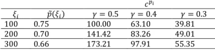
horizon (𝑇) 𝑝 𝑐𝑟 𝑐 0 ℎ 𝛾 𝑏 𝜓 𝑣 50 0.5 100 10 2.5 0.5 300 50 1 100 5 0.4 200 100 3 0.3 200 300 In this parameter setting, 𝑐𝑟 represents the acquisition cost of the regular supplier whereas 𝑐0 is the cost of printing without any laser polishing. In our numerical experiments, we consider three different laser energy densities which are 100, 200, and 300 J/cm2. For these energy densities, calculated total printing cost and reliability levels are given in Table 2 where 𝑝̃(𝜉𝑖) are calculated using parameters values 𝑎 = 3, 𝑟 = 0.01 and 𝑠 = −10−5 similar to the model suggested by Chang et al. [7].
Table 2: Calculated parameter levels for different laser
energy densities (𝜉𝑖) 𝑐𝑝𝑖 𝜉𝑖 𝑝̃(𝜉𝑖) 𝛾 = 0.5 𝛾 = 0.4 𝛾 = 0.3 100 0.75 100.00 63.10 39.81 200 0.70 141.42 83.26 49.01 300 0.66 173.21 97.91 55.35
For each parameter combination, the recursive equations (4) and (5) are numerically solved by the value iteration algorithm and backward induction [10] on a finite state space of 𝐐̅ × 𝐍̅, where 𝐐̅ = {(𝑞𝑡−1𝑟 , 𝑦 ): 0 ≤ 𝑞𝑡−1𝑟 ≤ 𝑁, 0 ≤ 𝑦 ≤ 𝐷𝑚𝑎𝑥𝜖 } and 𝐷𝑚𝑎𝑥𝜖 = max{𝑑: Pr{𝐷 ≥ 𝑑} < 𝜖}. In our calculations, 𝜖 = 0.001. Note that such a truncation of the demand distribution, which is also used by [11], is a simplification for avoiding the common problem of
curse of dimensionality in dynamic programming
solutions.
In these runs, we primarily observe the optimum control policy’s ordering decisions to the regular supplier, 𝑞𝑡𝑟, and printing decisions at quality level 𝑖, denoted by 𝑞𝑡𝑝𝑖
, for all 𝑖. Also, we are interested in the optimum selection of a quality level (optimum usage of laser energy density for polishing) for on-demand production of spare parts. In the following section, the structure of commonly observed control policy in our numerical experiments are presented.
3. Results
In our numerical investigation, we observe the effect of different model parameters on total cost as well as the structure of the optimal control policy for original parts inventory. In this section, we first present our overall results and intuition into the problem derived from these analyses. Next, we discuss the structure of the optimal policy.
522
3.1. Overall results
In our analysis, we find that cost of 3D-printing is the most important factor that determines the primary source of supply. Specifically, in our numerical experiments we find that when 𝛾 = 0.3 or 𝛾 = 0.4, the optimum action is to choose to satisfy spare parts demand using additive manufacturing. Interestingly, all of these parts are printed at the lowest quality level where laser energy density is set to 100. When 𝛾 is set to 0.3 or 0.4, total cost of producing a printed part is less than the original part as 𝑐𝑟= 100 (Table 2). When 𝛾 = 0.5, the combined use of printing and original parts takes place in the optimum policy. This can be seen in Table 3.
Furthermore, in all of our numerical experiments we find that the optimal cost is invariant to 𝑏 since on-demand production of spare parts prevents having an unsatisfied demand during the entire planning horizon (Table 3). This feature of the optimal policy is explained in detail in the following section.
Table 3: Average optimum costs for different values of 𝑏, 𝜓
and 𝛾. 𝒃 𝜸 200 300 0.3 0.4 0.5 𝝍 50 28509 28509 18177 28809 38541 100 28767 28767 18177 28809 39314 200 29201 29201 18177 28809 40616 300 29564 18177 28809 41707
Recall that the number of broken parts in a given review period is a random variable and the original spare parts inventory and 3D printing decisions are made according to a control policy. In the mathematical model given in (4-5), we consider a finite horizon cost minimization problem where decision for 𝑞𝑡𝑟 is followed by 𝑞𝑡
𝑝𝑖 for all 𝑖 . The mathematical structure of the optimum control policy is presented in the following subsections.
3.2. Structure of the optimum on-demand spare parts production
To understand the mathematical structure of the optimum printing policy, we conduct a mathematical analysis of the model in (4-5). The following result, obtained from these analyses, shows the optimum decision for 𝑡 = 𝑇 (the end of planning horizon).
Proposition 2: At the end of the planning horizon,
given that the total number of broken parts (from all quality levels) is 𝑑 ≔ 𝑑0+ ∑ 𝑑𝑣𝑖 𝑖, the optimal policy of
laser polishing is 𝑞𝑇 𝑝1
= (𝑑 − 𝑦)+.
Proof: Assume that 𝑉𝑇(. ) = 0 for all parameters.
For 𝑡 = 𝑇, 𝐺𝑇(𝐪̅𝐓+𝟏𝐫 , 𝑦𝑇, 𝑚0, 𝐦̿, 𝑑𝑜 , 𝑑̅𝑝) (7) = min 𝑞̅𝑇𝑝≥0, (𝑑𝑜+∑ 𝑑𝑖 𝑝𝑖−𝑦)+≥∑𝑣 𝑞𝑇𝑝𝑖 𝑖=1 {∑ 𝑐𝑝𝑖𝑞 𝑇 𝑝𝑖 𝑣 𝑖=1 + 𝐿 (𝑦, ∑ 𝑞𝑇𝑝𝑖 𝑖 , 𝑑𝑜+ ∑ 𝑑𝑝𝑖 𝑖 )} .
This implies for a given that the total number of breakdowns is 𝑑 the function in the minimization is:
∑ 𝑐𝑝𝑖𝑞 𝑇 𝑝𝑖 𝑣 𝑖=1 + ℎ(𝑦 − 𝑑)++ (𝑑 − 𝑦 − ∑ 𝑞 𝑇 𝑝𝑖 𝑖 ) + . (8)
If 𝑦 ≥ 𝑑, then the constraint of the minimization leads to ∑ 𝑞𝑇𝑝𝑖 𝑖 = 0 ⇒ 𝑞𝑇 𝑝𝑖 = 0, ∀𝑖. If 𝑦 < 𝑑, then minimization leads to ∑ 𝑞𝑇𝑝𝑖 𝑖 = 𝑑 − 𝑦. Hence, ∑ 𝑞𝑇𝑝𝑖
𝑖 = (𝑑 − 𝑦)+. Since the cost is increasing in 𝑖, 𝑞𝑇𝑝𝑖 > 0 is subotimal for 𝑖>1. Q.E.D.
Proposition 2 implies that the optimum policy prints parts from the worst quality level (no laser polishing) as it is the cheapest option. This result is quite intuitive in the sense that the end of the planning horizon, there is no point of increasing quality levels of parts in exchange of extra cost.
Importantly, we realized that the result in Theorem 1 also holds for periods before the end of the planning horizon, i.e. 𝑡 < 𝑇 in our numerical experiments. Our detailed investigation into our numerical results reveals that this result primarily stems from our assumption on the exchange of spare parts upon delivery of original parts together with uncapacitated (capacity equal to infinity [12]) OPS. In our system, spare part production with 3D-printing is used in case of the shortage of original parts during maintenance of capital products. Since we assume that OPS is capacitated, these shortages mainly occur due to unexpected spare parts demand in previous or current periods and they are rare. Also, delivery of original parts in pipeline triggers replacements. Therefore, in this system, 3D printing is used as a temporary solution to avoid costly downtimes of capital products and using laser polishing does not create any additional cost reduction.
3.3. Structure of the optimum order to OPS
Given that in case of shortage spare parts are printed after the demand realization, the control of original part inventory resembles to classical lost sales problem in the inventory control literature [13] depending on the magnitude of substitution cost. In lost sales problems, customers refuse to wait for delivery of products and leave without buying anything when they cannot find their desired product in stock. The inventory control decisions are made based on the trade-off between costs of lost sales and inventory holding. In our problem setting, printed spare parts stand for lost sales from the perspective
523 of the inventory manager of original spare parts. The cost of lost sales is equal to 𝑐𝑝𝑖 for some 𝑖. This equivalence between the lost sales problem and our problem setting can be seen from [14] for 𝜓 = 0. As an extra cost element of using 3D printing in case of shortage, 𝜓 significantly changes the structure of the optimal policy in our problem. To explore these changes, we extend the test bed in Table 1 with new parameter combinations of 𝜓 and 𝑏. We respectively present results of our numerical experiments for low and high values of 𝜓 below. In these expositions, we utilized the decomposition of the state space in Section 2. We first explained the optimal orders to OPS when 𝑦𝑡= 0 and 𝐦̅ ≠ 0. Next, we present the structure of the optimal policy when 𝑦𝑡> 0 and 𝑚0= 𝑁.
3.3.1. The optimum policy when 𝝍/𝒃 is close to 0
In case of low substitution cost, which is incurred due to replacement upon delivery, the summation of printing and substitution cost would be the cost of losing customer in a regular, single-supplier inventory control problem. The optimal control policy of this case has a state-dependent structure in the sense that the total amount of existing inventory level and ordered quantity, 𝑦𝑡+ 𝑞𝑡−𝑙𝑡𝑟 + 𝑞𝑡𝑟, also known as inventory position after ordering, is small for low values of 𝑦𝑡+ 𝑞𝑡−𝑙𝑡𝑟 and they are equal to base stock policy for moderate and large values of the summation. Note that the base stock policy is the optimum control policy for inventory control problems where unsatisfied demand is backlogged [12]. The optimal ordering policy to OPS places smaller orders than the base stock policy for low levels of inventory due to the fact that low inventory level leads to shortage which will be satisfied with 3D printing within the same period before the delivery of orders placed in the current period. On the other hand, in case of backlogged demand and a single supply source, where the base stock policy is optimal, unsatisfied demand is carried to the next period and keeps creating backlog cost until it is satisfied with new deliveries. This difference between the optimal orders to OPS for 𝑦𝑡= 0, 𝐦̅ ≠ 0 and the base stock policy is depicted in Figure 4 for 𝑣 = 3, 𝑇 = 50, 𝑏 =300, 𝜓 = 50, ℎ = 2.5, 𝛾 = 0.5 and 𝑁 = 10. In Figure 4, optimal 𝑞𝑡𝑟 for different 𝑦𝑡 levels are given for two different 𝐦̅ vectors which are (1,9,0,0) and (9,1,0,0). The first vector represents a case where only one of 𝑁 = 10 of machines works with an original part while the rest works with parts printed without laser polishing. The second vector represents the case with nine original and one printed parts. Obviously, the optimum policy generates the same orders with the base stock policy with the order-up-to level being equal order-up-to 21, which is denoted by 𝐵𝑆(21), when the existing inventory level is larger than equal to 10 for the first vector. For the second vector, the optimum policy is much closer to the base stock policy as the optimum policy generates the
same order sizes when the inventory level is larger than equal to 3. The difference between the two part vector is due to the fact that some of existing inventory level will be used to replace printed parts at work and remaining ones will be available for the satisfaction of broken spare parts within the review period when the number of printed parts at work is higher (as in 𝐦̅=(1,9,0,0)).
Figure 4. Difference between optimal ordering policy to
OPS and the base stock policy for 𝑣 = 3, 𝑇 = 50, 𝑏 =300, 𝜓 = 50, ℎ = 2.5, 𝛾 = 0.5, 𝑁 = 10, 𝑙𝑡 = 1, 𝑦𝑡= 0 and 𝒎̅ ≠ 0.
When there is a positive amount of original spare parts in stock (and all capital products are working with original parts 𝑁 = 0), the structure of the optimal policy is much closer to the base stock policy as depicted in Figure 5. In fact, when there are some parts in the pipeline (𝑞𝑡−𝑙𝑡𝑟 ), the optimal policy orders exactly the same with 𝐵𝑆(12). When there are no parts in the pipeline, the optimal policy is also the same with 𝐵𝑆(12) except 𝑦𝑡= 0.
Figure 5. Difference Between Optimal Ordering Policy to
OPS for 𝑣 = 3, 𝑇 = 50, 𝑏 =300, 𝜓 = 50, ℎ = 2.5, 𝛾 = 0.5, 𝑚0= 𝑁 = 10 and 𝑙𝑡 = 1, 𝑦𝑡> 0 and 𝒎̅ = 0.
3.3.2. The optimum policy when 𝝍/𝒃 is close to 1
When 𝜓/𝑏 is close to 1, then the structure of the state-dependent optimal policy significantly changes. When the original part inventory is empty 𝑦𝑡= 0 and 𝐦̅ ≠ 0, the optimal policy behaves differently depending on the value of 𝑡 and 𝑞𝑡−𝑙𝑡𝑟 . During the early periods of the planning horizon (𝑡
𝑇< 0.75) , the optimum policy is similar to the concave decreasing curve given in Figure 4, i.e. order according to 𝐵𝑆(. )
524 for large values of 𝑞𝑡−𝑙𝑡𝑟 and order less than 𝐵𝑆(. ) which we call correction due to printing. In case of 𝑦𝑡> 0 and 𝐦̅ = 0, the structure of the optimal policy is also the same with Figure 5 for different values of 𝑦𝑡. Towards the end of the planning horizon (0.75 ≤𝑡
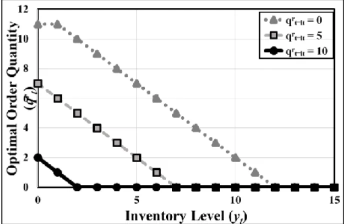
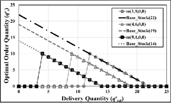
𝑇), the optimum policy orders nothing to OPS for low value of 𝑞𝑡−𝑙𝑡𝑟 whereas orders according to BS for moderate or large values of 𝑞𝑡−𝑙𝑡𝑟 . As can be seen in Figure 6, ordering threshold depends on the number of printed parts at work. When there is one printed part in the system, the optimal policy orders according to 𝐵𝑆(14) for 𝑞𝑡−𝑙𝑡𝑟 ≥ 4. When the number of printed parts is equal to nine, then ordering with 𝐵𝑆(12) takes place for 𝑞𝑡−𝑙𝑡𝑟 ≥ 12 (Figure 6).
Figure 6. Optimal Ordering Policy to OPS for 𝑣 = 3, 𝑇 = 50,
𝑏 =300, 𝜓 = 150, ℎ = 2.5, 𝛾 = 0.5, 𝑁 = 10 and 𝑙𝑡 = 1, 𝑦𝑡= 0 and 𝒎̅ ≠ 0.
Dependence of the optimal policy on the remaining number of periods is also depicted in Figure 7 for 𝐦̅ = (1,0,0,9). Towards the end of the planning horizon, orders to OPS significantly decreases in the optimum policy and production of spare parts using additive manufacturing becomes the main source of spare parts in the system.
Similar to Section 3.3.1, when there is a positive amount of original parts in the system, the structure of the optimal policy is much closer to 𝐵𝑆(. ) as in Figure 5. There is only a minor correction in case of 𝑞𝑡−𝑙𝑡𝑟 = 𝑦𝑡= 0. The rest of the orders are linearly decreasing in the inventory position before ordering, i.e. 𝑞𝑡−𝑙𝑡𝑟 + 𝑦𝑡.
Figure 7. Optimal Ordering Policy to for 𝑣 = 3, 𝑇 = 50,
𝑏 =300, 𝜓 = 150, ℎ = 2.5, 𝛾 = 0.5, 𝑁 = 10 and 𝑙𝑡 = 1, 𝑦𝑡= 0 and 𝒎̅ = (1,0,0,9).
4. Discussion and Conclusion
In this study, we consider a problem setting where spare parts can be produced on-demand using additive manufacturing at a location very close to the working site of a finite number of capital products. Capital products require regular maintenance in order to stay in operation and spare parts are the primary input of these maintenance activities.
Recently, additive manufacturing, specifically 3D printing, is shown to be quite beneficial for spare parts inventory control as it allows on-demand production of spare parts instead of ordering them to OPS [9]. Since such orders are usually delivered after a positive lead time, maintenance companies have to hold spare parts inventory in order to avoid long downtimes of capital products which might lead to loss of customers or failure to satisfy service commitments.
The main drawback of using printed spare parts is that they usually fail quicker than the original ones. This is due to their less favorable mechanical properties, and in particular, fatigue life. A factor significantly affecting reducing fatigue life and thus reliability of a product is surface quality. Therefore, improving surface quality of printed parts can mitigate the difference in reliabilities of original parts and printed parts. Laser polishing has been shown to be a quick and effective method to improve surface quality of printed parts by reducing the surface roughness through eliminating surface waviness caused by the staircase nature of 3D printing process. However, effectiveness of this post-production technique has been shown to be significantly affected by its technical parameters such as laser energy density, a factor that is dependent on laser scan speed and laser power [8]. From the perspective of manufacturing economics, laser polishing is a technique that can increase the reliability of a spare part in exchange of an additive cost of polishing. Hence, parameters of laser polishing (laser power & speed) are decision variables which should be optimized together with other cost elements.
In this study, we consider the problem of joint optimization of inventory management and laser energy density selection in order to decrease the total cost of holding, printing, polishing, and downtime costs. To this end, we develop a recursive, two-stage mathematical model that aims to minimize total discounted cost over a finite planning horizon. We utilize this mathematical model in order to develop exploratory analysis of optimum control policies which are difficult to prove mathematically. Furthermore, we numerically analyzed the effect of having multiple laser energy density level on total cost and control policy. In these analyses, we find that having multiple levels of laser density has no effect on total cost, since in the problem setting spare parts
525 are replaced with their originals upon delivery from OPS before their failures. Such a preventive replacement strategy might be plausible for mission critical systems such as military sites or aircraft carriers.
Importantly, the sum of exploratory analyses and results presented in this study is an initial step towards rigorous mathematical proofs for optimum control policies of a manufacturing/inventory system consisting of additive manufacturing, laser polishing, and inventory control elements. In our future research, we concentrate on deriving analytical characterization of the numerical results presented here.
References
[1] Bellini, A., Güçeri, S. 2003. Material Characterization of Parts Fabricated Using Fused Deposition Modeling. Rapid Prototyping Journal, 9(4), 252-264.
[2] Pandey, P.M., Reddy, N.V., Dhande, S.G. 2003. Improvement of Surface Finish by Staircase Machining in Fused Deposition Modeling. Journal of Materials Processing Technology, 132(1-3), 323-331.
[3] Lee, K., Jee, H. 2015. Slicing Algorithms for Multi-Axis 3-D Metal Printing of Overhangs. Journal of Mechanical Science and Technology, 29(12), 5139-5144.
[4] Ding, D., Pan, Z., Cuiuri, D., Li, H. 2015, A Multi-Bead Overlapping Model for Robotic Wire and Arc Additive Manufacturing (WAAM). Robotics and Computer-Integrated Manufacturing, 31, 101-110.
[5] Ma, C.P., Guan, Y.C., Zhou, W. 2017. Laser Polishing of Additive Manufactured Ti Alloys. Optics and Lasers in Engineering, 93, 171-177.
[6] Maiya, P.S., Busch, D.E. 1975. Effect of Surface Roughness on Low-Cycle Fatigue Behavior of Type 304 Stainless Steel. Metallurgical Transactions A, 6(9), 1761.
[7] Chang, C.S., Chen, T.H., Li, T.C., Lin, S.L., Liu, S.H., Lin, J.F. 2016. Influence of Laser Beam Fluence on Surface Quality, Microstructure, Mechanical Properties, and Tribological Results for Laser Polishing of SKD61 Tool Steel. Journal of Materials Processing Technology, 229, 22-35. [8] Perez Dewey, M., Ulutan, D. 2017. Development
of Laser Polishing As an Auxiliary Post-Process to Improve Surface Quality in Fused Deposition Modeling Parts. ASME 2017 Proceedings. https://doi.org/10.1115/MSEC2017-3024. [9] Westerweel, B., Basten, R., den Boer, J., van
Houtum, G.-J. 2018. Printing Spare Parts at Remote Locations: Fulfilling the Promise of Additive Manufacturing. Working paper. Eindhoven: Eindhoven University of Technology. [10] Bertsekas, D.P. 1995. Dynamic programming and optimal control, Vol 1. Athena scientific. Belmont, MA.
[11] Hekimoğlu, M., Van der Laan, E., Dekker R., 2018, Markov-Modulated Analysis of a Spare Parts System with Random Lead Times and Disruption Risks, European Journal of Operational Research, 269 (3), 909-922.
[12] Porteus, E.L. 2002. Foundations of stochastic inventory theory. Stanford University Press. [13] Zipkin, P. 2008. On the structure of lost-sales
inventory models. Operations Research, 56(4), 937-944.
[14] Sheopuri, A., Janakiraman, G., Seshadri, S. 2010. New Policies for the Stochastic Inventory Control Problem with Two Supply Sources. Operations Research, 58(3), 734-745.