i·· Чмі/
*^Т ">'ЧТ‘ Г>Т7 ■" -:^> г г?-· г f г :-г гг.'^-л. ^ '^ ■ ψт^:·.г rv.'^'S*
A SIMULATION STUDY TO DETERMINE
RAW MATERIAL SAFETY STOCKS AND PRODUCTION BATCH SIZES
MBA THESIS
GÖKŞİN YILMAZ ANKARA, JANUARY 1995
η
I certify that I have read this thesis and that in my opinion it is fully adequate, in scope and in quality, as a thesis for the degree of Master of Business Administration
Assist. Prof. Erdal EREL
I certify that I have read this thesis and that in my opinion it is fully adequate, in scope and in quality, as a thesis for the degree of Master of Business Administi'ation
Assist. Prof. Murat MERCAN
I certify that I have read this thesis and that in my opinion it is fully adequate, in scope and in quality, as a thesis for the degree of Master of Business Administration
Assist. Prof. limit Yl'JCEER
i ly ^ I
Approved by Dean of the Graduate School of Business Administration
Prof. Dr. Siibidev TOGAN
/
ABSTRACT
A SIMULATION STUDY TO DETERMINE
RAW MATERIAL SAFETY STOCKS AND PRODUCTION BATCH SIZES
Gökşin Yılmaz MBA
Supervisor: Assist. Prof. Erdal Erel January, 1995, 81 pages
MRP II controlled production systems are large in scope and generally complex in operation. Consequently the total time required to fill a customer order through procurement and production activities is very long. This study proposes a method to increase the throughput of a real MRP II controlled production system by using the data available in the system. Critical raw materials and subassemblies of a product are determined by using project scheduling techniques. A simulation model is developed by using SIMAN. Simulation experiments are performed for determining raw material safety stock quantities and production batch sizes with the objective of decreasing the time required to fill a customer order.
Keywords : Material Requirements Planning (MRP), Manufacturing Resource Planning (MRP II), Work-in-Process Inventory (WIP), Accumulated Lead Time (ALT). Critical Path Method (CPM)
ÖZET
HAMMADDE GÜVENCE STOKLARI VE ÜRETİM KAFİLE BÜYÜKLÜKLERİNİ BELİRLEMEK İÇİN BİR BENZETİM ÇALIŞMASI
Gökşin Yılmaz MBA Yüksek Lisans Tezi
Tez Yöneticisi: Yrd. Doç. Dr. Erdal Erel Ocak, 1995, 81 sayfa
Üretim Kaynak Planlaması (MRP II) kontrollü üretim sistemleri, işlev alanı olarak geniş ve genellikle işlemsel olarak karmaşıktır. Sonuç olarak saunalma ve üretim işlevleri aracılığıyla müşteri talebini karşılamak için gereken süre çok uzundur. Bu çalışma, MRP kontrollü, ger çek bir üretim sisteminin çıktısını, sistemdeki verileri kullanarak arttırmayı amaçlayan bir yön tem önermektedir. Belirli bir ürünün kritik hammadde ve alt takımları proje çizelgelemesi yön temleri kullanılarak belirlenmektedir. SIMAN kullanılarak bir benzetim modeli geliştirilmekte dir. Müşteri talebini karşılamak için gereken süreyi düşürmek amacıyla, hammadde güvence stoklannı ve üretim kafile büyüklüklerini belirlemek için benzetim deneyleri gerçekleştirilmek- tedir.
ACKNOWLEDGMENT
I would like to thank Assist. Prof. Erdal Erel for his invaluable supervision throughout this thesis. I would also like to thank Assist. Prof. Murat Mercan and Assist. Prof. Ümit Yiiceer for their help. I owe a great debt to the following colleagues and friends: Şule Anil, Utku Akça, Sezer Kadayıfçılar, Oğuzhan Peksarı, Leyla Demir, Richard HaiTİson and Russell Fraiser. Special thanks go to my wife, Nuray, for her lifelong support and patience.
TABLE OF CONTENTS
1. INTRODUCTION ... 1
1.1. OBJECTIVE OF THE THESIS ... 1
1.2. OUTLINE OF THE THESIS ... 1
1.3. HISTORY OF M R P... 2
1.4. EVOLUTION OF MRP II SYSTEMS ... 3
1.5. MRP II IN ASELSAN COMMUNICATIONS GROUP (ACG) ... 5
1.6. MANUFACTURING PROCESS ORGANIZATION IN ACG ... 8
2. SIMULATION ... 12
2.1. INTRODUCTION ... 12
2.2. CHARACTERISTICS OF THE SYSTEM UNDER STUDY... 14
2.2.1. PUSH SYSTEM... 14
2.2.2. LOT FOR. LOT POLICY... 15
2.2.3. EQUALITY OF TRANSFER AND PROCESS BATCHES... 15
2.2.4. PROCUREMENT FOR TOTAL NEED... 16
2.2.5. INFINITE LOADING ... 18
3. METHODOLOGY... 21
3.1. ALT ANALYSIS FOR THE PRODUCT ... 21
3.2. SIMULATION STUDY... 24
4. EXPERIMENTATION ... 37
4.1. DETERMINING THE PRODUCTION BATCH SIZE ...37
4.2. DETERMINING RAW MATERIAL SAFETY STOCK QUANTITIES ... 40
4.3. ANALYSIS OF DEMAND VARIATION ... 45
4.3.1. CHANGES IN DEMAND SIZE ...47
4.3.2. CHANGES IN INTERARRIVAL TIME OF DEMAND ...50
5. CONCLUSIONS ...53
5.1. CONTRIBUTIONS OF THIS STUDY ...55
5.2. FURTHER RESEARCH ITEMS ... 55
REFERENCES ... 58
1. INTRODUCTION
1.1. OBJECTIVE OF THE THESIS
This study uses real life data from a firm where MRP II was first installed in 1991 and a severe purchasing problem is routinely observed. A product, which is a representative of the product mix, is chosen. We will concentrate on a solution for the purchasing problem: Holding safety
stocks of the most critical items whose procurement times contributes an important amount to the accumulated lead time. Accumulated lead time can be defined as the total time
required a make part in stock if none of the components in its product structure is in stock.
The advantage of holding safety stocks is the decrease in the time required to fill a customer de mand. Inventory holding cost that will occur in relation to the safety stock quantities is the dis advantage of this policy. As a result, we will attempt to establish a U'ade-off between inventoiy holding cost of the average inventory kept and the time required to fill a customer demand in response to different safety stock quantities. We will also attempt to derive the production
batch size that will minimize the time required to fill a customer demand.
Our tool in this study will be simulation which is the appropriate tool in this complex and sto chastic environment. This will be done for a single product, but may be repeated for other prod ucts and their critical raw materials.
1.2. OUTLINE OF THE THESIS
This thesis is organized as follows: Chapter 1 is introduction to MRP II and to the firm under study. The tool. Simulation, and the characteristics of the simulation study are briefly explained in Chapter 2. Chapter 3 contains the methodology and anticipation of inventory holding cost for the firm. The experimentation starts with Chapter 4. Chapter 5 is devoted to the conclusions and further research items.
1.3. HISTORY OF MRP
Around 1958, some manufacturing companies began to use computers to solve their problems of the inability to get the right information on a timely basis. Computers began to be used as a possible tool to manage production and inventory. The most popular methods in production and inventory control imitated the manual techniques using the power of the computer to handle large quantities of data and perform many simple arithmetic calculations without human error. These types of efforts became known in the late 1960s as Material Requirements Planning (MRP). The classic textbook on MRP technique is by Orlicky (1975). The technique had been manually practised in aggregate form prior to the Second World War in several locations in Eu rope. What Orlicky realized was that computers enabled the detailed application of the tech nique, which would make it effective in managing manufacturing inventories of dependent items. (Browne,et.al.,1989)
Similar to many other areas in computer business, IBM was a pioneer in developing an integrat ed set of basic application programs which depended on the Bill of Material and routing ap proach. Goldratt (1988) discusses that the customary separation between bill of materials (BOMs) and routings is not obligatory. His investigation led him "to believe that this separation stems from the fact that the early attempts to build an MRP system were done when computer disks were not available and computer tapes were the only media available to store volimunous data." When a common subassembly was used in many different assemblies, combination of routing and BOM would "pay the price of punching the same information many times" and the user would "lead to unavoidable discrepancies and mistakes" by updating the same information in multiple entries.
Tlie developers chose "repeating the bill of materials of the subassembly but storing its routings only once." In contrast "when computer disks appeared, these problems disappeared." Unfortu nately at this stage consolidation of those two files was very hard since too much was already invested in the method of storing BOM and routing data separately.
Even MRP II (Manufacturing Requirements Planning) concepts and practices aie not veiy new. They have evolved from the lessons learned with early MRP (Material Requirements Planning) systems developed in the 1960s. By today's standards, those early MRP systems seem archaic, lacking many of today's common features.
In the early 1970s, MRP's power to improve control over manufacturing companies was heavily publicized. In USA, the American Production and Inventory Control Society (APICS) launched the "MRP Cmsade" to promote the benefits of MRP. In reality the basic concepts of MRP were established in the early 1960s by a few individuals attempting to implement systems. The con cept of time series, level by level planning based on exploding the bill of material against a known future demand was recognized as a more rational approach than the classic reorder point (ROP) system, which determined when to order from historical data. The problems asso ciated with ROP systems were numerous and these systems could not answer the question: "When do we need it?"
Related to the increase in the crunching power of computers, IBM offered the first commer cially available softwai’e package in the mid 1960s and provided the first written material and educational classes on MRP. The number of firms implementing an MRP package increased quickly, and the first firm in the commercial MRP (and later MRP II) software market,IBM, became the leader with COPICS^ and MAPICS^. (Goldi'att, 1988)
1.4. EVOLUTION OF MRP II SYSTEMS
As time passed, the installations of the technique have become more widespread and vaiious operational functions have been introduced. These extensions have included Master Production Scheduling (MPS), Production Activity Control (РАС), Rough Cut Capacity Planning (RCCP), Capacity Requirements Planning (CRP), and Purchasing.
ing) with the potential for feedback from the execution cycle to the planning cycle, was termed closed loop MRP. The addition of financial modules, extension of MPS and the support of busi ness planning in financial terms, has resulted in an integrated system for management of manu facturing resources. This extended MRP is known as MRP II today. Since 1980, MRP applica tions have been adapted on mini and micro computers.
Some authors describe MRP II as follows;
"MRP II is a closed loop MRP system with additional features to cover business and financial planning as depicted in Figure 1." (Browne,et.al.,1989)
"The development of a sound, workable production plan requires the integration of marketing, financial, product development, and manufacturing objectives and activities. This integration, which provides consistency and coordination vertically throughout an organization from top management to the production worker, describes what is meant MRP II." (John, 1986)
DEMAND MANAGEMENT PURCHASING BOM CONTROL INVENTORY CONTROL PRODUCTION PLANNING RESOURCE REQUIREMENTS I PLANNING | r ROUGH CUT CAPACITY PLAN. MASTER PRODUCTION SCHEDULING MATERIAL REQ. PLANNING
PRODUCTION ACTIVITY CONTROL DISPATCHING IINPUT/OUTPUT C.
FIGURE 1: MODULAR STRUCTURE OF MRP II SOURCE: (Browne,et.al.,1989)
1.5. MRP II IN ASELSAN COMMUNICATIONS GROUP (ACG)
ASELSAN Communications Group (ACG) is the biggest division among three divisions which exist within the structure of ASELSAN A.§. (Organizational Structure of ASELSAN A.§. is given in Appendix as Exhibit 1.) In ACG, MRP II was first installed in 1991. Mainly the in crease in variety of products produced, and the number of subassemblies and raw materials created the need for installation of MRP II software.
Before installation of MRP II in ACG, there were three types of computer systems in use. These were VAX, IBM/System 44, and PC's used within departments.
These computer systems were not connected via a network; each of them worked independently and data transfer between them was impossible. Even within the same computer system, data integrity and security was unavailable.
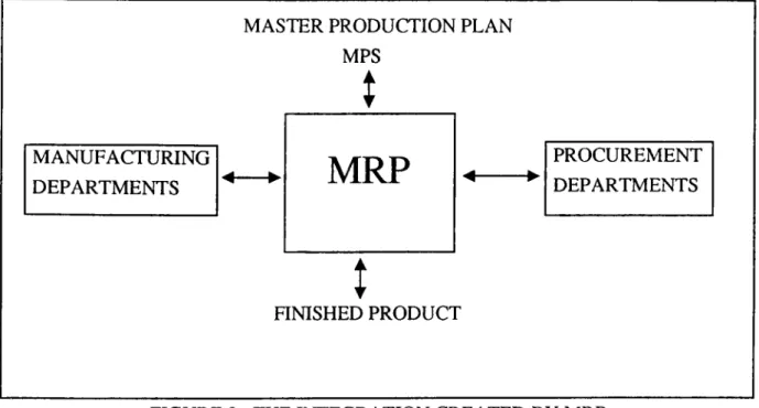
The same data were stored in different systems with different formats. Thus it was difficult for a depaitment to benefit from other departments' data ba.se systems. Before MRP II installation. Computer System / Data / User of the System connection was not well established. Managers understood that MRP was a formal system which would create the integration depicted in Figure 2 in a reliable manner.
The installation of an MRP package was however insufficient, the information flow within de partments which was ambiguous and informal, also needed to be emphasized. A foimal Input / Output Information structure was a need for ACG. As a result, MRP II is considered to be the appropriate tool to create system integration and to form a closed loop system as in Figure 3.
Some typical prejudices may be obseiwed during the installation stage when a company decides to install an MRP II software package :
i) Much of the firm's attention and efforts ai'e focused on MRP's technical aspects, such as the kind and size of the computer hardware, programming techniques, and the file sizes used for
MASTER PRODUCTION PLAN MPS
i
MRP
MANUFACTURING DEPARTMENTS PROCUREMENT DEPARTMENTS ^ Wi
HNISHED PRODUCTFIGURE 2 ; THE INTEGRATION CREATED BY MRP
FINANCE
MARKETING ◄---►
MRP II
◄---► DEVELOPMENTPRODUCTPRODUCTION
storing data. In many cases, too much focus on these aspects can lead to underestimating plan ning, management and the human issues of installation.
ii) Installation of MRP II without planning all elements and subsystems.
iii) Performing the installation process through personal efforts, rather than using project man agement techniques for management of the process.
iv) Obtaining MRP II software before planning the installation procedure, and before investing
in a focused, planned program of education and training.
v) Lack of top management's total commitment and support before implementation.
These factors may be clearly recognized by middle managers as typical prejudices against a successful MRP II installation. Top management total commitment was lacking in 1987 when ACG bought the current MRP II softwai'e. For four years the installation process mainly de pended on personal efforts. In 1991, these initial biases were solved by forming an implementa tion team, focusing on education, U'aining and using project management techniques.
The implementation process was completed at the end of 1991; making ACG one of the first successful implementers of MRP II in Turkey. Today some companies considering to imple ment an MRP II software can benefit from ACG's experiences, and ACG is willing to provide the companies all the technical help in the process of implementing.
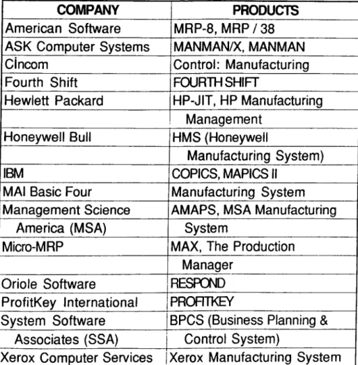
The installation of an MRP II system was a major change within ACG. The main objective of this installation was to create an integrated system joining together marketing, accounting, production, engineering, and finance departments. MRP II software is selected from a leading firm in MRP II software market: ASK Computer Systems Inc. (Major MRP II Software prod ucts are listed in Appendix Table 1.) The software works on Digital Equipment Corporation's VAX system. The general name of the software package is MANMAN containing mod ules such as MFG (Manufacturing), SY (System), OMAR (Order Management. Accounts
Receivable), and REPETITIVE.
1.6. MANUFACTURING PROCESS ORGANIZATION IN ACG
In terms of manufacturing process organization, ACG has a pure jobshop system which con tains the following characteristics:
i) Low volume production runs of many different products.
ii) Very low level of standardization.
iii) Flexible production capability, flexible equipment capable of performing many different tasks.
iv) A highly skilled work force.
v) A hybrid system of order processing which mainly depends on make to order inventory poli cy and also on a smaller volume of make to stock.
Related to job shop system, ACG has a production flow policy which uses work order schedul ing instead of repetitive manufacturing. ACG has some existing and potential products which could be produced with repetitive manufacturing principles, but current layout and work center organization eliminates this possibility.
MANMAN has a separate module (MANMAN/REPETITIVE) to perform repetitive manufac turing policy tasks which depend on build schedules instead of work orders. This module is not used in ACG.
Today MRP II plays a very important role in ACG, but the results are similai· to other compa nies where a complete closed loop MRP II system could not be achieved. Late orders, hot and shortage lists are observed by everyone in the firm. Beginning in 1993, a performance measure
ment and management reponing system acts within ACG and results show that ACG is not cur rently a CLASS A MRP II company. In many cases, the problems are observed to be interrelat ed with purchasing problems. Everyone agrees that there exists a severe purchasing problem, additionally other problematic areas exist which are discussed as follows:
i) A big variety of products within the product mix: ACG produces 500 different products which contain different configurations assembled according to customer orders and expecta tions. This level of variety creates a lack of focus, but is consistent with the company's goal of "being national and producing whatever is expected by the Turkish army and civilian fimis (mainly public institutions) in terms of electronic products and services."
ii) Being mostly dependent on foreign suppliers: This situation mainly affects fixed lead times of purchased materials. ACG's foreign suppliers, some of which are transnational companies such as Philips, TDK, Aztech, Sumitomo, are much bigger and stronger than ACG. As a result ACG's bargaining power is (or is supposed to be) much less than that of these suppliers. We know that in general a new order goes to the end of the vendor's queue of orders; most of the lead time is consumed waiting in line. A customer can significantly shorten the lead time by buying capacity from the vendor. In this approach, the customer determines the priority for the purchased capacity and eliminates competition for priority in the vendor's shop. Since major suppliers are bigger firms and materials purchased are veiy diverse (i.e. focus on distinct ven dors seems to be infeasible), ACG tries to live with very long fixed lead times for purchased
materials.
iii) The Turkish legal system is very strict on imported materials. ACG's dock to stock lead times (which mainly contain the time from customs to the firm) are long, with an average of 9 days due to this inflexibility.
iv) Difficulty in making long term forecasts and planning related to the instability ot Turkish economy.
v) Since a formal vendor performance measurement system has not been set up, all purchased materials undergo inspection on aixival: Studies on a vendor performance measurement system continues and this will create a new policy in which purchased materials from reliable vendors will not undergo inspection on arrival. Today the average time passed in incoming inspection is 4 days.
vi) Lack of project management and team work experience: Especially in the new product de velopment stage, this problem is observed and steps are taken to eliminate. Although concur rent engineering principles are supposed to be implemented with the pressure of TOTAL QUALITY CONTROL, which top management has had a high commitment to since 1993, the concept is fairly new. Recently, teams containing middle managers have been set up during product development stages, but we could not obtain any information on whether or not project management techniques, which depend on milestone checks, ai'e formally used in these stages.
vii) Lack of a formal employee performance measurement system: A "Performance Evaluation Sheet" is filled in for every employee once a year, but feedback from these evaluations is not given to employees. A formal performance measurement system depending on positive rein forcement is an important need of ACG.
Other problematic ai'eas can be added to this list, but there is a consensus that the main problem is a purchasing problem such as:
i) Percentage of work orders kitted with shortages is, on average, 22.62 % (see Exhibit 2.)
ii) Percentage of purchase orders delivered before or on the need date is, on average, 65.46 % (see Exhibit 3.)
The purchasing problem which makes the people accept the statement: "Our major problem is purchasing with very long lead times and long shortage lists." also becomes the bairier for what can be done on the shop floor and in marketing.
Related to the globalization process, the main competitors of ACG, especially in terms of ex port, are transnational companies. The major strength of ACG is that ACG is a national firm which makes contracts on businesses related to Turkey's national security, with the Turkish Go- verment and Army, the most important customers for ACG products. If the issues of national security and supporting a national firm begin to be underemphasized by major customers, com petition from transnationals such as Marconi and Motorola may hurt ACG to an unexpected de gree. As a result, ACG has to overcome the problem of purchasing and concentrate on market ing and shop floor.
There are some problem areas on the shop floor and development opportunities to overcome these problems. As examples, material handling systems are not well organized, typical job shop layout causes time wasting with long transit, queue, set-up and quality conu'ol times. A manufacturing organization depending on manufacturing cells could lead to higher productivi ty and employee satisfaction. There are some existing and potential products which could be produced with repetitive production methodology and production lead times could be de creased with formation of assembly lines. All these development opportunities must be ana lysed and evaluated, and this should be worked out at shop floor level.
2. SIMULATION
2.1. INTRODUCTION
A simulation is the imitation of the operation of a real-world process or system over time. The facility or process of interest, which is a collection of entities, such as people or machines which act and interact together toward a logical end, is called a system. The behaviour of a sys tem as it evolves over time is studied by developing a simulation model. In the formation of the model we make some assumptions concerning the operation of the system and express the mathematical, logical, and symbolic relationships between the entities, objects of interest, of the system. After development and validation of a model, it can be used to investigate what if questions about the real world system.
Simulation can be used to determine the effects of a potential change planned to make within the system or it can be used as a tool to study systems in the design stage. If simulation inputs are changed and the resulting outputs are investigated, the most important variables for the sys tem can be determined and the interaction between these variables can be evaluated.
When a model is simple enough to react to what if questions by mathematical methods, it is suggested to solve these questions by the use of differential calculus, probability theory, alge braic methods etc. Simulation is a tool for complex and dynamic systems whose analysis is too hard with the use of mathematical methods.
With all these characteristics, the popularity of simulation in OR/MS and in daily applications within factories increased very rapidly. The following impediments to simulation's wider accep tance have been eased in recent years:
i) Not too long ago, a mainframe computer was needed to do serious simulations. Now there exist simulation packages that pack the power of big computer simulation into a desktop com puter.
ii) Model developing for lai-ge systems which needed large-scale computer programs was a hard task. This difficulty disappeared with the development of several special-purpose computer lan guages such as GASP, SIMSCRIPT, GPSS, and SLAM. New commercial packages which are more popular for factory operations, have been evolved. Examples of this new software are SIMAN, ProModel, Taylor, XCell and Factor/Aim. Packages which rely on graphics and win dows have made them easy to use.
iii) For large systems, a large amount of computer time is required, but the cost of computing steadily decreases, especially in comparison with the benefits obtained.
iv) The use of animation in simulation studies made simulation the most appropriate tool in ob taining top management commitment especially for new designs.
Simulation models are generally classified as:
i) Static or Dynamic: A static simulation model is a representation of a system at a particular time. (Monte Carlo simulations). A dynamic simulation model is the representation of a system as it evolves over time; such as simulation of a work hour of an emergency room.
ii) Deterministic or Stochastic: A deterministic model has no random variables, so it has a unique output for every input. A stochastic model has random variables such as interamval times, so the output of the model is also an estimation of the true characteristics of the model, such as service rate for airiving customers.
iii) Discrete or Continuous: A discrete system is one in which the state variables, such as the number of orders waiting for process, change only at discrete points in time. A continuous sys tem is one in which the state variables, such as the water level in a dam, change continuously over time. Although few systems can be evaluated as wholly discrete or continuous, the one dominating the system is accepted to determine the classification of the model.
discrete.
2.2. CHARACTERISTICS OF THE SYSTEM UNDER STUDY
The simulation study on an MRP II controlled product will reflect a complete MRP environ ment. The characteristics of this environment are as follows.
2.2.1. PUSH SYSTEM
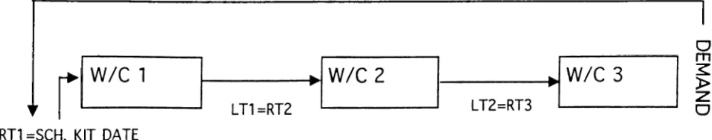
The operation of MRP on the shoop floor is mainly a push system. For example, a subassembly produced in a push system, should pass three work centers, say W/C 1, W/C 2, and W/C 3. When the demand for that subassembly occurs, the raw material for that subassembly is first as signed to W/C 1 on the assembly's scheduled kit date (release time for W/C 1), with a due date to transfer to W/C 2. This due date is the release date for W/C 2. The same procedure follows for W/C 3 (Figure 4).
This study assumes that the airival of a customer demand initiates production with a signal to the first processing work center. This is one of the characteristics of the Constant WIP (CONWIP) production lines. CONWIP has an additional characteristic: A job is not started un less there is a place in the system for that job. In the system under study, there is not such a control. The absence of this characteristic indicates that the system is mainly a push system.
RT1 =SCH. KIT DATE O m > z o LT3=SCH. DUE DATE
2.2.2. LOT FOR LOT POLICY
This system uses the common order policy in MRP practice. It is the direct translation of net re quirements into order quantities. We use this policy for ordering raw materials and try to derive production batch of the product by using simulation. As an example, if a raw material of the finished product (an item only appears once in the BOM of the finished product) has a quantity per assembly value of 2 and the demand for the product equals 10, then we will order 20 units of this item from the vendor.
If the stated item is a routable subassembly produced by the company, and if a decision to pro duce the finished product with a batch size of 2 is made, then:
1. We will have 5 batches for the finished product to fulfill the demand size of 10.
2. We will also have 5 batches for the routable subassembly and the batch size for subassembly will be 4.
2.2.3. EQUALITY OF TRANSFER AND PROCESS BATCHES
One of the main criticisms of MRP scheduling is of equality of process and transfer batches. Especially as Optimized Production Technology (OPT) philosophy, initiated by Goldi'att and Fox and considered by Vollmann (1986) as an enhancement to MRP II, gained popularity, traditionally discouraged lot splitting and overlapping began to be discussed.
Browne et. al. (1989) discuss that there are at least two lot sizes to be considered in manufac turing:
1. The transfer batch: lot size from the parts point of view.
By differentiating these lot sizes, a firm can make better scheduling which will result in shorter lead times. We can describe the difference between transfer and process batches more clearly- with the following example: When transfer batch equals process batch, any items within a batch of 100 units will not be moved to the following work center until all of the 100 units are proces sed in that work center.
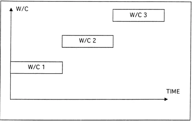
Since we make an analysis on a product scheduled using MRP techniques, differentiation be tween transfer and process batches is beyond the scope of this study. We will assume that a product produced with a flow from W/C 1 to W/C 2 and from W/C 2 to W/C 3 will have a schedule like the one in Figure 5.
If transfer batch is not equal to process batch, then a better schedule as in Figure 6 may be ob tained with a marked reduction in throughput time.
2.2.4. PROCUREMENT FOR TOTAL NEED
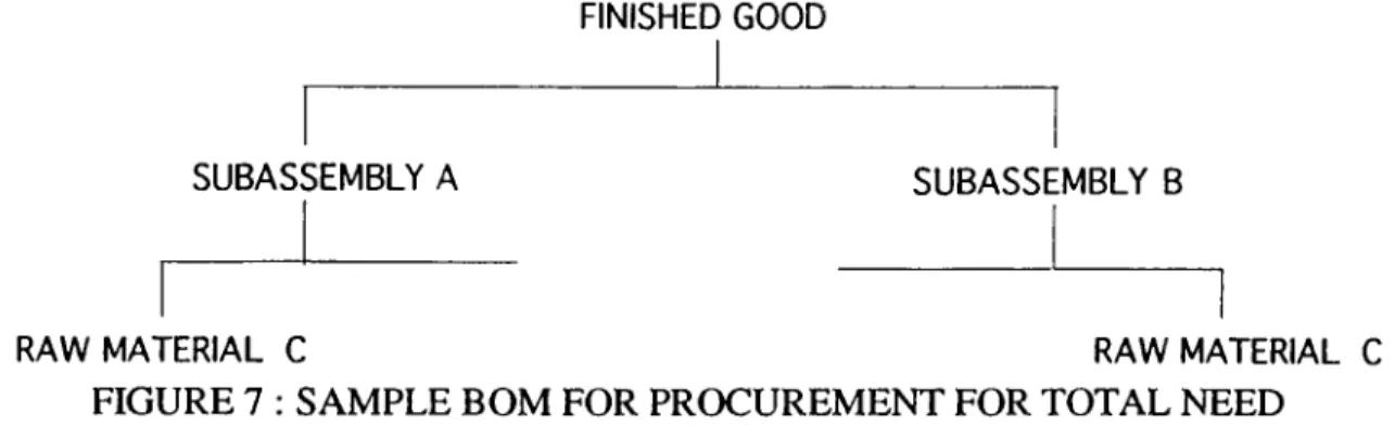
If the situation in Figure 7 occurs within the BOM structure of the finished good, then the pur chase order quantity of Raw Material C will include both the need for Subassembly A and Sub- assembly B. To maintain this, MANMAN has an option of "Number of Days Supply" figure among the informations entered in the system for a part. MANMAN adds up all requirements for a part within the number of days supply range.
FIGURE 5: Schedule when Process Batch = Transfer Batch
FINISHED GOOD
SUBASSEMBLY A SUBASSEMBLY B
RAW MATERIAL C RAW MATERIAL C
FIGURE 7 : SAMPLE BOM FOR PROCUREMENT FOR TOTAL NEED
2.2.5.INFINITE LOADING
MRP is designed as a system which can handle large quantities of data and perform many sim ple calculations without human error. This made MRP a simple tool in terms of capacity plan ning. The capacity planning concept of MRP relies on infinite loading. Goldratt (1988) discuss es that "The second approach (as an alternative to MRP) was much more ambitious and tried to use mainly the computational power of the computer to reach a more precise answer for a shop floor scheduling system. This approach was based on detailed schedules of the shop floor tak ing into account the finite capacity of all its machines. In the mid 1960s this approach became known as 'finite scheduling' and its stronghold was in West Germany."
Finite loading technique is mainly a shop floor technique. It, more than any of the other capaci ty planning techniques, makes clear the relationship between scheduling and capacity availabil ity. Finite loading starts with a specified capacity level for each work center or resource group ing. This capacity is then allocated to planned orders. Alternative work centers on routings are evaluated when a work center is fully utilized. As a result finite loading is a method for sched uling work orders.
MRP systems generally have a module (or subprogram) called as CRP (Capacity Requirements Planning.) It uses the infinite loading principles to determine work load on resources a follows;
i) CRP utilizes the information produced by the MRP explosion process, which includes con sideration of all actual lot sizes as well as the lead times for both open shop orders and orders that are planned for future release.
ii) The gross to net feature of the MRP system takes into account the production capacity alre ady stored in the form of inventories of both components and assembled products.
iii) The shop-floor control system accounts for the current status of all WIP in the shop. As a re sult the capacity needed to complete the remaining work on shop orders is considered in calcu lating the required work center capacities.
iv) CRP takes into account the demand for service parts, other demands that may not be acco unted for in the MPS, and any additional capacity that might be required by MRP planners re acting to scrap etc.
As an MRP tool, MANMAN/MFG is developed with the same fallacies, used mainly in any MRP system. As a Rough Cut Capacity Planning (RCCP) tool, MANMAN/MFG has several commands which are called Resource Requirements Planning Tools. To test or "rough cut" a production schedule, one needs to define the critical resources within the production system. Critical Resources are those resources that are both crucial to the manufacturing of the product and limited in nature with potential to cause backlogs in workflow. Critical resources can inclu de trucks for shipping, warehouse space, and machines with limited capacity.
In MANMAN/MFG how each critical resource is to be used is defined by bills of critical reso urces which are similar structures to bills of materials.
After critical resources have been identified, their usages and a production plan are entered into the system, a Resource Requirements Planning report is obtained to evaluate the daily and cu mulative weekly load of the resource. With the help of this report, planners should validate the production plan by:
i) Rescheduling some workload on overutilized cridcal resources.
ii) Refusing some workload if overutilization cannot be managed with overtime, increase in the number of the shifts etc.
iii) Deciding to increase capacity of critical resources such as workspace, critical machines.
iv) Modifying the production plan in advance of potential bottleneck situations.
After RCCP is run and MPS is validated, CRP options of MANMAN/MFG enable one to deter
mine the availability of labor and machine hours at each work center for a given period of time. Using this information, one can plan the best utilization of each work center's capacity.
MANMAN/MFG's capacity planning feature is based on infinite loading. Capacity planning re ports both work center machine and labor loads, but in cases of overloading, do not indicate where to shift work.
In our study, the infinite loading feature of an MRP system will be accepted and used. This ac
ceptance will lead us to the following conclusions:
1. Capacity of resources used within the production system will only be limited by the number of shifts (one shift for ACG) and consequently by the total number of working hours of the system (8 hours per day in ACG.)
2. When an activity that requires a resource, reaches that resource, it will be assumed that the required resource is dedicated to that activity. Following this assumption, to seize a resource for an activity will only be constrained if the activity which requires that resource is not a newco mer i.e. that resource has already been seized by the same kind of activity before.
3. As a result, utilization of a resource will be determined by the operation lead times related to that resource.
Shortly, our simulation model which tries to determine the condition in an MRP environment will be insensitive to scheduling problems and will assume that the system works in an envi ronment consisting of dedicated work centers (resources.)
3. METHODOLOGY
In this study, we will recommend a solution for purchasing problems in ACG: Holding safety stocks of the most critical items whose procurement times contributes an important amount to the accumulated lead time (ALT). We will find out the amounts of these critical materials to be stocked and derive the best production batch for a product.
The product chosen has a part number of 5820-4510-0012 in ACG, which is "Hand Radio 6-25 KHz." This product has a complex BOM consisting of 8 levels, 189 purchased raw materials, and 44 subassemblies produced within ACG.
The product has mainly two printed circuit boards, but other mechanical and electronical subas semblies are also needed to build up the product. This is a typical and representative product for ACG's product mix.
5820-4510-0012 does not have a smooth demand pattern like many other products of ACG (see Exhibit 4.)
3.1. ALT ANALYSIS FOR THE PRODUCT
ALT analysis study began in the Production Planning and Control Depaitment of ACG at the end of 1993. The reason for this study was that all the products produced in ACG had long ALTs as a characteristic. (This study was presented in XVI. National OR/IE Congress.)
ALT is defined as: The total time needed for production of a product, beginning with procure ment of raw materials and ending with ti'ansfer of the finished product to finished goods inven- toiy if all the raw material and subassembly inventories of that product are zero.
ALT is mainly used as:
Demand Time Fence can be described as the time interval in which production plan of a product should be stable.
2. The easiest and most common information that determines the delivery date that can be offered to the customer in a make-to-order production environment.
ALT is a crucial information in the integration of Production and Marketing in an MRP II envi ronment
The "ALT Analysis" study have become an important tool for revision and updating of this cru cial information within ACG.
In this study, we described the BOM structure of a product as a network. All the nodes in the BOM structure are assumed to be the activities of the network structure. Activity durations are:
i) Fixed procurement lead times for purchased materials.
ii) For subassemblies, the time is calculated as follows:
Fixed Lead Time + (Variable Lead Time * Average Order Quantity)
Once the network is established, CPM analysis on this network determines the critical path for the project duration (ALT for this study). Concentrating on these paths makes the process of revising and updating of ALTs an easier task.
The method used for ALT analysis in ACG may be described as follows:
i) A computer program is developed by the Information Processing Department. This program uses the information stored in MANMAN/MFG, and describes BOM structure of a product as a network.
ii) The products which need ALT analysis urgently are determined. One of the products is 5820-4510-0012, the product under consideration.
iii) Critical paths are determined for a product by using CPM and the required raw materials which take place in the beginning part of critical paths, are analysed. Consequently, reduction of fixed procurement lead times of the raw materials under consideration and several alternating approaches are being attempted;
-Renegotiating with suppliers of these raw materials on new and (possibly) shorter lead times.
-Investigating for alternative suppliers of critical purchased materials.
-Considering to make long term contracts with reliable suppliers of critical raw materials.
iv) Searching ways to minimize the non-value adding times such as transportation, set-up, queue and quality control for subassemblies on critical paths of the finished product.
v) After the possible reductions on non-value adding times, operation times of these subas semblies will be investigated for reduction.
The common characteristics of the study in ACG and this thesis aie the following items which are evaluated in both:
i) When fixed procurement lead times of raw materials cannot be decreased to a level that will make a path noncritical, then it is proposed to stock these materials in the raw material inven tory in an amount with no (long-lasting) shortages allowed whenever a demand occurs to the fi nished product. We will derive the safety stocks of critical raw materials for the product, 5820- 4510-0012, in this study.
ii) The simulation study tests the effect of setting different values for the decision vai'iable, pro duction batch size. The batch size which minimizes the total time required to fill a customer or der, will be the Average Order Quantity of ALT analysis.
The critical raw materials and the production flows in which the raw materials are consumed to produce the required subassemblies of 5820-4510-0012 are presented in Appendix as Exhibit 5.
We can think of this flow as a simplified network of the product.
The raw material safety stock quantities and production batch size will be determined through the simulation of the process flow on this network.
3.2.SIMULATION STUDY
The simulation language, SIMAN, is used in this study. It is a registered product of Systems Modeling Coiporation. It was first introduced in 1983 and has been improved continuously to include several new features since then.
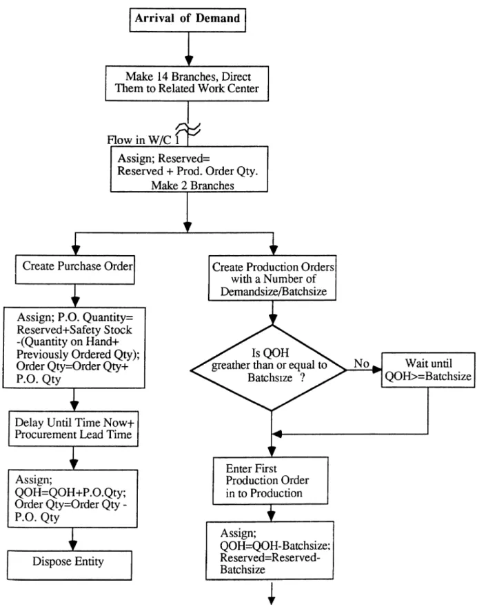
The simulation process initiates a flow by a customer demand for the product. The demand size, which is stochastic, is truncated to the nearest multiple of the batch size. Tliis truncation is not obligatory, but makes the simulation process easier. The demand becomes the push signal for production of the subassemblies of the final product. Occurrence of demand initiates an entity. The entity is branched to the raw material procurement stations.
A purchase order is created in a raw material procurement station with a delivery date consist ing of fixed procurement lead time for this raw material. This information is stored in MAN- MAN/MFG database, and fixed procurement lead times are estimated with a normal distribu tion with a variance of 5 days in the simulation study. The purchase order quantity should cover the raw material need to fill the demand which has just occun'ed and the needs for other de mands which are waiting to be produced in the first work center at the instance. Safety stock quantity of the raw material is added to this amount. The quantity in raw material inventory and the quantity ordered before are subtracted to derive the net amount that will be ordered from the supplier.
When enough data are unavailable to anticipate the demand pattern for a product, the opinion of the experts can be an effective anticipation tool. The project planner's opinion for the product
under consideration is that interarrival time of the demand can be estimated with an exponential distribution with mean, 800 (unit is hours, approximately an arrival in every 100 days.) De mand size can be estimated with a uniform distribution with minimum and maximum values, 2(Ю and 300 respectively. This indicates that demand sizes and interarrival times will be subject to important variations throughout the simulation experiments. This level of variation in de mand size and interarrival time is usual for the products in ACG's product mix. We will also an alyse the model performance in changes of accepted demand pattern.
If the sufficient amount of raw material is available in the inventory, the production center begins to produce that batch size. If the quantity on hand is insufficient to produce the batch size, production is delayed until the quantity on hand increases to an amount that will cover the batch size with the arrival of a purchase order. Batch size is a policy parameter, hence deter mines whether or not a production starts.
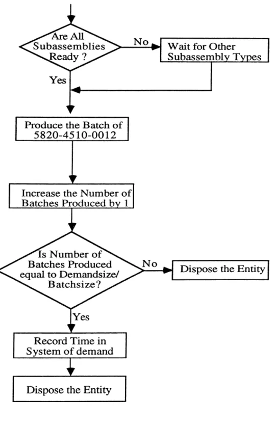
The batch follows the routing and waits for other subassemblies required to complete the finished product, 5820-4510-(Ю 12, as WIP inventory. Production flows of subassemblies are derived from the routings stored in the MANMAN/MFG database. Process durations are de rived from the routing standard set-up and operation times. The flow chart of the simulation model is presented in Figure 8.
To find out distribution of standard set-up and operation times, we make use of the literature about this subject. Muralidhar, Swenseth and Wilson (1992) analyzed the effect of the selection of processing times in simulations on production lines. In their studies, truncated normal, gamma and log-normal distributions are used. Although they concentrated on the pull produc tion systems, use of their results in this study will not cause serious errors.
The results show that the selection of the distribution of the processing times make no signifi cant difference in performance of the production line. However gamma distribution is recom mended for describing the processing times since it satisfies the requirements and it is computa tionally efficient.
I
MEAN = ALPHA/BETA VARIANCE = ALPHA / BETA^ where ALPHA is the shape parameter.
BETA is the scale parameter.
Coefficient of variation (CV) of gamma distribution becomes only a function of ALPHA:
CV =
(V
VARIANCE)/ MEAN= fVaLPHAI / BETA = 1 /VALPHA ALPHA/BETA
Lau and Martin (1987) studied how a production line's utilization factor could be affected by a variety of shapes for the stations' processing times (i.e. skewness and kurtosis). They state that several researchers use a convenient distribution such as the normal, but empirical investiga tions have shown that actual station-processing times cannot be adequately estimated by a nor mal density function since there is a variety of shapes possible.
Lau and Martin conclude that for a 10-station line with no buffers, the eiTor incuned is roughly 3.5 % if the processing times of all stations have CV = 0.2, ALPHAl = 2 and BETA2 = 6. This represents about the worst case for a 10-station line. Smaller errors will occur if buffers exist, the CV is lower and the line is shorter.
Since observed deviation from MANMAN routing standard times in ACG is about 20% of the MANMAN value (see Exhibit 6 in Appendix), we will use the same CV used by Lau and Martin.
In our test runs, we studied 3 different distributions for standard set-up and operadon times:
1. Gamma disdibution with a CV of 0.2.
MEAN = ALPHA * BETA
VARIANCE = ALPHA * BETA^.
We make mean equal to MANMAN routing standard time and standard deviation equal to 20% of the MANMAN routing standard time in this study. Thus,
BETA = 0.04 * (MANMAN routing standard time)
ALPHA = 25.
2. Exponential distribution with mean and standard deviation = routing standard time.
3. Normal distribution with mean = routing standard time;
standard deviation = 0.2*(routing standard time).
Normal and gamma among these three distributions seem to fit the current situation in ACG. Exponential distribution with the high CV value, results in big variations and instable flow times within the system. This contradicts the current situation in ACG. As a result, we decided to follow the recommended distribution: gamma. In fact the results obtained by gamma and normal distributions are very close to each other i.e. we can conclude that Muralidhar, Swens- eth and Wilson's statement is validated in our test runs.
Data for the performance measure, time required to fill a customer demand, are collected when all the units to fill the customer demand are produced. After the duration in terms of hours is taken into statistics, the entity created at the start of the simulation flow by the occuixence of the customer demand is disposed.
This model is run for different safety stock quantities of raw materials and also for different production batch sizes.
In this study, we want to estimate the system's performance during the steady-state phase. Any observations recorded during the transient phase will bias our results. We aie modeling a job- shop and we begin the simulation in the empty and idle state, the initial jobs will amve at an uncongested system with idle machines and zero stock levels. Hence, the early arriving jobs will wait for aixival of purchase order, but will quickly move through the idle machines. After the system warms up, we will have non-zero inventories, queues in the shop-floor. As a result observations collected after the warm-up period will be representative of steady state behavior.
Our method used to deal with the initial bias problem is to discai'd those observations recorded during the transient phase of the simulation. This approach necessitates selecting a truncation point, t, at which all previous observations are discarded.
The simple and practical method for selecting the truncation point is visual determination, i.e., selecting the ti'uncation point from a plot of the simulation response over time. To achieve this, we made long simulation runs. We observed that the most important bias occurs because of the initial zero stock levels. After the first purchase orders which cover the demand and safety stock quantities ai'e purchased, this bias disappears.
Exhibit 7 in Appendix is the time in system data obtained with a simulation run where safety stock quantities of all raw materials equal a huge number (10,000) and production batch size equals 40. The number of fulfilled demands is 2,000 and statistics collected during the produc tion period of 10 initial demands ai'e discarded. Raw time in system data ai’e processed by using a moving-average filter to smooth the fluctuations in the response. The moving-average is con structed by calculating the average of the most recent observations at each data point in the data set. If we increase the moving-average size (50 in this case), we can increase the "smoothness" of the response.
Analysis of the plot of the diagram indicates that transient phase bias in this study can be elimi nated by discarding some of the initial demands. (We discai'd the first 10 demands.) There is not a trend in the simulation results and time in system data vary due to congestion of ma
chines. The jobs that airive at a congested system create a high time in system value while the jobs that anive at an uncongested system quickly move through idle machines. This implies
that time in system data mainly depend on the interarrival time of the demand.
To determine the simulation run length, we make different simulation runs with different lengths. The results imply that a simulation run containing 2,000 fulfilled demands takes about 50-60 minutes while a simulation run of 800 demands takes only 15-20 minutes. Comparison of results show that there is not a significiant difference between the results of the 2,000 fulfilled demands case and the latter. Consequently we make simulation runs which end with fulfillment of 800 demands.
In addition to these, we make 4 or 5 different simulation replications (a modest sample size from a statistical viewpoint) for different combinations of our variables. The term "run" is used throughout the simulation study to indicate that a simulation experiment is performed by changing the value of the decision variables. The term "replication" means that a simulation experiment is performed without changing the value of the variables, but with a different ran dom number stream. The aim of performing several replications is to eliminate the biases that can occur due to the use of the same random number stream in each case. If we want more pre cision for a decision variable, we make a higher number of simulation replications, such as 10 and 20.
3.3. ANTICIPATION OF INVENTORY HOLDING COST
"Holding (Carrying) cost" is the amount of money the company must invest to continue carry ing the inventory time after time. Even if inventory is expensed when it is received, the compa ny has still lost the use of the money. Company would have to borrow the money in order to buy the inventory if the company did not have excess money. Tlie cost of borrowing money is one of the prime ingredients in inventory carrying costs.
At least, inventory on hand costs the company as much as what the firm could get if the money was deposited in a bank account (opportunity cost of the money tied in inventory.)
Prime ingredients of carrying cost elements may be summarized as follows:
1. Equipment Depreciation and Maintenance: Book depreciation for material handling equip ment.
Many of the material handling equipment, still used in ACG's warehouse operations are fully depreciated, so their yearly depreciation figures are zero. There exists some new equipment such as a forklift, but the accounting department gives the information that yearly depreciation figures for this equipment will be available at the end of 1994.
Using the principle of "Any estimate is better than none", yearly depreciation calculated by using straight line depreciation will be:
ACQUISITION COST / EXPECTED LIFE TIME = 140,000,000 (TL)/ 10 (years) = 14,000,000 TL/year
2. Electiicity: Costs for individual areas located in inventory storage areas.
Electricity is used for illumination of the storage ai'eas and for usage of computer terminals. There exist 350 lamps, each of which consumes 40 watts an hour and 4 terminals which con sume 260 watts an hour.
ELECTRICITY USED FOR ILLUMINATION / YEAR =
40*350*8*240 = 26,880,000 watl/year (number of work days in a year = 240)
ELECTRICITY USED FOR TERMINALS / YEAR = 260*8*240 = 499,200 watt/year
TL VALUE OF ELECTRICITY USED / YEAR = 2400 (TL/KW)*27380 (KW/year) = 65,712,000 TL/yeai·
3. Stock Handling: Wages paid to receiving personnel, warehouse supervisors, clerical help, all involved in stock handling.
Gross wages paid to warehouse personnel have a total monthly figure of 145,000,000 TL.
GROSS WAGES PAID / YEAR = 145,000,000*12 = 1,740,000,000 TL/year
4. Breakage and Obsoloscence: Cost incurred for breakage, loss by employees and obsoles cence due to expected life cycle.
Lost inventory account has a yearly total of 164,000,000 TL. No data is available about ob solescence.
5. Building maintenance services.
The warehouse is totally maintained in 3 year cycle with operations such as painting the walls, repair of the broken equipment, and renewal of electrostatic discharge sensitive materials. This maintenance costs about 300,000.000 TL, so the yearly estimate is 100,000,000 TL.
6. Building depreciation and / or rent.
The building is not depreciated and belongs to ACG, so there is not a rent payment.
7. Fuel oil used with several purposes such as heating of inventory storage areas.
Heating cost of a square-meter is about 11,335 TL per month. The total warehouse ai'ea is 1400 im, as a result;
HEATING COST/YEAR = 11,335*1400*12 = 190,428,000 TL/year
8. Taxes and insurance paid for inventory.
Data about taxes are unavailable, additionally we know that insurance is not paid for inventory.
9. Cost of Money:
9.1. Rate of Opportunity Cost
We can estimate total opportunity cost as:
TOTAL OPPORTUNITY COST =
MONEY VALUE OF INVENTORY HELD * REAL INTEREST RATE
In estimating real interest rate, we must consider about how to get the best return on the money spent for procurement in alternative investments. The usual method is to refer to treasury bills or goverment bonds, but in Turkey this will not be a reasonable approximation since return of these investments usually vary speculatively in a wide range according to changing political/ec- onomical condition. Thus, a reliable estimator is a new investment policy of Turkish banks offering a rate of return to compensate inflation plus an additional 10 percent, can be a more reliable estimator.
1 YEAR'S RETURN = 1 + NOMINAL INTEREST RATE (N) = 1 + INFLATION RATE (F) + 10
1 YEAR'S REAL RETURN = (1 + N) / (1 + F) REAL INTEREST RATE = ((1 + N) / (1 + F)) -1
= 10/(1 +F)
Assuming an inflation rate of 100 %
9.2. Corporate Lending Rate
ACG does not usually borrow money in order to buy the inventory. ACG finances the procure ment activities with the obtained from sales. We cannot make any approximation about the lending rate for the obligatory situations when sales' return is unavailable to finance the pro curement activities.
We can summarize the carrying cost elements from which we derived yearly figures, in Table 1. Money tied up in inventory in the last 13 months is presented in Table 2.
As a result, TL value of average stock kept in inventory is 120,850,000,000. The ratio, TL VALUE OF HOLDING COST ELEMENTS
TL VALUE OF AVERAGE STOCK
will give us the holding cost of 1 TL. This ratio is 0.02.
Adding real interest rate to this figure as the opportunity cost of holding 1 TL inventory will re sult in inventory cost of holding a unit (1 TL) inventory for a year.
T A B L E 1 ; T H E C A R R Y IN G C O S T E L E M E N T S COST OF (Million TL) Equipment Depreciation 14.00 Electricity 65.71 Stock Handling 1,740.00 Breakage 164.00 Building Maintenance 100.00 Heating 190.43 TOTAL= 2,274.14 TABLE 2
RAW MATERIAL INVENTORY MONTH-END TOTAL STANDARD COSTS (Billion TL)
OCT. 1993 104.00 NOV. 1993 80.00 DEC, 1993 70.00 JAN, 1994 70.00 FEB, 1994 70.00 MAR, 1994 101.00 APR, 1994 102.00 MAY, 1994 121.00 JUN, 1994 130.00 JUL, 1994 152.00 AUG, 1994 166.(X) SEP, 1994 173.00 OCT, 1994 232.00 AVERAGE 120.85
T A B L E 3 ; T IM E IN S Y S T E M IN R E S P O N S E T O B A T C H SIZ E S PRODUCTION B S’l CH SIZE R E P n —
iSEEDTT
REPT2 (S'EED2)KEP.3 REP. 4 XVERACE TIME IN
"2ir ID" (SEE1T3T ■82F.38" (SEED 4) 850.68 SYSTEM (HOURS) 82833 3 9 6 3 0 ' 740.22 "4D" 663.18 671.06 661.13 650.92 "661.57 3 (r w 647.50 689.62 "688:4r 703.26 637.72 '710.19 "66832" 708.52 660.59
■7D23D"
"593:95 706.28 700.89 313779" 719.66 708.07■7TT
■718.19 780.28 "9(r 786.66 723.95 789.03 721.72 753.44 717.54 777.35 "8n779" ■7 7 2:2 3· 759.00 803.26 ■m .37" K K r TUT ■T2(r■83733"
822.05■86D3T
'78739· 854.66 857.37 838.23 806.46"83232"
818.27 799.77"93832"
924.04802.41 825.08"8T9.98"
811.81 "HIT 9IT29· 944.70 952.78 999.29 931.56 969.04 3 4 (r 330" 967.25 964.90 l,oo6.0o ""9897)2" i,0O9.80 ■9 9 0.7 3“ 990:3 9· 1,009.60 1,003.95 360" '973:94· "99736" 1,073.00 1,007.50 1,006.83 i;002.40 T7(r I W 1,005.50 999.44 993.84 963.89 989:02 950.97 1,011.50 9 5 9.3 3· 1,000.72 956.36 --- T90---BATCH = DEMAND 1,008.50 '•9 5 1:2 2“ 1,217.00 1,177.9(7 1,201.68 1,209.50" 1,202.30 4. EXPERIMENTATION4.1.DETERMINING THE PRODUCTION BATCH SIZE
In order to determine the production batch size, we treat production batch size as a variable, independent of the other variables, safety stock quantities. We set safety stock quantities to a huge number such as 10,000. Our performance criterion is the average time required to fill a customer order (time in system) and with this safety stock quantities there will not be any material shortages when a demand occurs (except the first demand whose time in system is discarded in the performance calculation stage.) This implies that the only variable that deter mines the performance criterion, time in system, is production batch size. Results obtained with 4 different initial seeds (with different random number streams) are given in Table 3.
In Figure 9, the plot of time in system values, observed according to different initial seed values and different production batch sizes, is given. The first observation is that production batch siz es of 30 and 40 give us nearly the same time in system values. To decide if there is really a sig nificant difference between these two batch sizes, we make 6 more replications with these batch
ю о оо О Г-о ѴО О О о СП О < S U Û о оо О Г-· о 40 о о TJ-О СП о CN ш 2 р ш О у;
ί |
< 00 СП Д и m g І-Н H в Q S Pu, C/D S ω C/D CN Û ö c/o û Ш w ό 00 N HH 00 Œ m O H Щ СЛ Z O CL, c/o m δ s [ii 00 ?H СЛ 2 h-H ω Os D o HH Uu (Nsize figures. Results are summarized as follows:
Batch Size 30
Time in System (hours) 663.66
40 666.07
We can conclude that production batch sizes of 30 and 40 make the system fastest in response to customer demand and the difference between these two production batch sizes is not signifi cant.
Master production planners in ACG often enter a customer order directly into the master production plan (MPS) unless the demand size is extraordinarily big. The MRP process then uses the quantity in MPS to explode requirements to all lower levels of the product structure. This kind of lot sizing policy is called "lot for lot". Even when lot for lot policy does not require big batches of the subassemblies in the product structure, production planners prefer to produce in big batches to fill customer orders expected to occur in the near future. Consequently batch sizes smaller than 50 are rare in ACG.
We know that change in a system should be evolutionary as a result of continuous improve ments. Hence, the analysis indicates that 40 is the best production batch size for the lot sizing policy of 5820-4510-0012. This production batch size requires an average time of 666 hours on the shop floor to fill a customer order. The common lot sizing policy used in ACG, lot for lot, yields the worst results for this product.
An intuitive explanation that describes what may happen when a production system works with small batches is provided in Goldratt’s famous book. The Goal (1992, revised edition). Goldratt explains that "set-up and process are a small portion of the total elapsed time for any part. But queue and wait (the time the part waits, not for a resource, but for another part so they can be assembled together) often consume large amounts of time -in fact, the majority of elapsed total the part spends inside the plant." He concludes that "If we reduce batch sizes by half, we also reduce by half the time it will take to process a batch. That means we reduce queue and wait by
half as well."
These explanations are also valid in our case. The tendency in ACG to work with high batch sizes is mainly ascribed to high set-up times. In this model the highest set-up time is equal to 19.54 hours, when the resource of this operation is occupied by a former batch with a batch size of 40, the queue time for a new coming batch is equal to 53.46 hours. Increase in the batch size will increase the queue time in the following manner:
Batch Size Queue Time (hours)
50 60 70 100 61.94 70.42 78.9 104.34
This queue time will have a direct impact on wait time of a batch which will wait for this batch, so they can be assembled together. We can conclude that working with small lots is also effec tive in this case and results in lower time in system values since small batch sizes decrease queue and waiting times by a considerable amount.
4.2. DETERMINING RAW MATERIAL SAFETY STOCK QUANTITIES
To determine raw material safety stock quantities, we implement the same method which we used in determining the production batch size. We fix safety stock quantities of raw materials except one, then change safety stock quantity of the exceptional material and observe the im pact of this change in our performance measures: mainly time in system and holding cost of av erage inventory kept in stock as a secondary measure.
Prior to this operation, we state the lower (best) and upper (worst) bounds of time in system values for different safety stock quantities.
10 simulation replications, when safety stock quantities are set to a very high value such as 10,000, reveal that the lower bound for time in system is 666 hours. Another group of 10 repli
cations with zero safety stock quantities yields 771 hours as the average time in system.
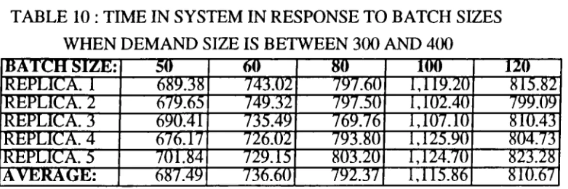
We also analyse system's performance when safety stock quantities are much lower than 10,000. In this way we decrease the range of our analysis. Assigning safety stock quantities of all raw materials as 1000, 500 and 300* results in the time in system values presented in Table 4. Figure 10 shows a plot of these results.
The result shows that assigning safety stock quantities to 300 yields an acceptable average time in system, but the average inventories are high, consequently inventory holding cost is high. (See Table 5.) We can take 679 hours as a local best of the average time in system and decrease
safety stock quantities to lower levels with the aim of approaching our local best, 679.
Nine of the sixteen raw materials have high standard prices and usage rates on the shop floor. As a result the other performance measure, average inventory holding cost, is mainly derived from them.
Sorting these raw materials according to their prices results in Table 6.
Our method for decreasing these materials' safety stock quantities to more acceptable levels is to decrease the safety stock figure of only one material from 300 to 250, then from 250 to 200 and so on, till safety stock quantity reaches zero (a total of 6 runs for every decision variable) while safety stock figures of all other materials are kept constant. We try to attain our local best 679 while we decrease the safety stock quantities. When we decide on the safety stock quantity of a raw material, we also keep this quantity constant as we study on other materials.
In each run, we make four simulation replications to eliminate the bias because of the use of the same random number stream in each case. Effort is concentrated on raw material safety stock quantity of 5905-9995-5032 since it has the highest standard price.
*: Since the raw materials, 5950-3000-0003.5950-3000-0002 and 6811-3007-1940 are used in different subassemblies, their safety stock quantities are different from the stated values. For 0003 and 0002, safe ty stock quantities are three times and for 1940 twice the stated values.
T A B L E 4
T IM E IN S Y S T E M I N R E S P O N S E T O S A F E T Y S T O C K L E V E L S
SAFETY STOCK REP. 1 REP. 2 R EP.3 REP. 4 AVERAGE TIME
QUANTITY* (SEED 1) (SEED 2) (SEED 3) (SEED 4) IN SYSTEM (HOURS)
1000 649.50 664.83 662.05 688.35 666.18
500 696.02 692.63 687.33 691.88 691.97
300 666.03 707.67 669.51 673.35 679.14
0 720.99 882.41 736.84 728.47 771.00
* : AVG. TIME IN SYSTEM OF ZERO SAFI3TY STOC LEVEL]S AVG. OF 10 RUNS
FIGURE 10