Linear filtering for a class of jump processes arising in navigation systems

linear Filtering for a Class of Jump Processes Arising in Navigation

Systems T. E. DABBOUS

Department of Electrical and Electronics Engineering, Bilkent University, Ankara, Turkey

S. S. LIM AND N . U . AHMED

Department of Electrical Engineering, University of Ottawa, Ottawa, Canada [Received 19 June 1989 and in revised form 2 March 1990]

In this paper, the filtering problem for a class of jump processes with discrete observations is considered. Using a minimum variance approach, a linear recursive unbiased filter is obtained with the help of which the required estimate and the corresponding covariance can be determined. The proposed filter allows multiple jumps for the state process, thereby making the theory applicable to modern navigation problems (Omega and Loran-C receivers), where multiple jumps have been reported to be a common occurrence. Further, utilizing the filter equations, the question of continuous dependence of the filter on system parameters is studied. Finally, a numerical example based on a navigation system model is presented, to illustrate some of the results of this paper.

1. Introduction

IN THIS paper, we consider the filtering problem for a class of systems governed by a linear stochastic differential equation of the form

dx{t) = A(t)6t + o(t)dW(t) + Cdr1(t) ( f e / = [0,T]), x(0) = xo, (1)

where A, a, and C are given matrices of appropriate dimensions, x0 is a Gaussian

random variable, and W is an n-dimensional Wiener process independent of x0.

The process {r/(f) : fSsO}, which is independent of x0 and W, is a temporally

homogeneous Markov chain taking values from some finite set. The observation process is given by

y(tk) = H(tk)x(tk) + [V(tk) - V('*-.)] (k = 0, 1, 2,..., N),

where V is another Wiener process independent of x0, W, and r/, and

{tk : 1 =£kssTV} is a finite set i n / » [ 0 , r ] such that 0 = to<tt< ••• <tN = T. At

each discrete time point tk, we have the observation y(tk) as given above. Our

problem is to give an unbiased minimum variance estimate of the process {x{t) : 12*0}, given the history {y(tk) :l^k^N}.

This problem has been treated in the literature for a special class of jump processes where r\ is only allowed to have single jump [3, 9]. Here we consider more general situations admitting multiple jumps for the process T/, thereby making the theory applicable to modern navigation problems (Omega and

269

2 7 0 T. E. DABBOUS, S. S. LJM, AND N. U. AHMED

Loran-C receivers) where multiple jumps have been reported to be a common occurrence [10].

It is clear from equation (1) that, owing to the presence of the jump process r\, the classical Kalman filter cannot be applied to this problem. In this paper, we develop filter equations that work and give estimates far superior to those obtained by use of a Kalman filter that ignores the presence of jumps. However, as we shall see, if the jump sizes are small, one can ignore the jump process r\ and use a Kalman filter with confidence. On the other hand, if the jump sizes are large, one has to modify the Kalman filter equations so that the effect of these jumps is included in the estimator and covariance (matrix) equations. This fact is clearly indicated in Section 3.

The paper is organized as follows. In Section 2, we formulate the filtering problem and present the necessary assumptions and notation. In Section 3, we use the results of [14] to derive the corresponding filter equations. In Section 4, we utilize the results of Section 3 to study the question of continuous dependence of the filter on system parameters. Finally, in Section 5, we develop an algorithm for computing the required estimate and present a numerical example, which is based on the navigation model developed in [10], to illustrate the effectiveness of the proposed filter.

2. Formulation of filtering problem, notation, and assumptions

In navigation problems [3, 9, 10], the process to be estimated is governed by a system of stochastic differential equations of the form

dxc(t)=A(t)xc(t)dt + o{t)dW(t) ( r e / = [0,r]), xc(0)=xco, (2) and

(teJ), xd(0) = xdo, (3)

where A e R"x", a e R"*', and C e Rm x r. The initial states xc0 and x% are assumed

to be Gaussian random variables (independent of W and r/) with certain mean and covariance. The process {W(t) :teJ) is an /-dimensional Wiener process satisfying

E{[W(t) - W(s)][W(t) - W(s)]T} = f Q(d) dd (s ^ t),

where Q is a positive definite matrix valued function. The process {r/(f) : t eJ}, which is independent of x0 and W, is a temporally homogeneous Markov chain

taking values from a finite set 21™ {elt elr..,eM} c W with transition probability

matrix S{t) = {Sq(t): i,j = 1, 2,..., M} (t s= 0) satisfying the following (matrix) differential equation

| ( / e / ) , 5(0) = /, (4) where / denotes the identity matrix. The matrix A denotes the infinitesimal

generator of the Markov chain with elements {A/p/: i,j = 1, 2,..., M}, given by

for i #y,

K,=

We assume that the elements

lim S,,(t)lt '10

lim (Sv(t)-l)It for i=j.

satisfy the following property: fory = i - l , i + 1,

M k+i

(5)

0 otherwise.

As indicated earlier, a similar class of systems was considered in the literature for filtering navigation signals [3, 9]. For this system, the proces TJ was assumed to satisfy a stochastic differential equation of the form

dr/(0 = l ( r / ( r ) = 0)Nt(dt) - l ( r / ( r ) = l)N2(dt), (6)

where 1(X) denotes the indicator function of the set X and Nt and N2 are two

independent Poisson processes with certain mean. Assuming a discrete observa-tion model, the authors in [3, 9] have used a minimum variance approach to derive a linear unbiased filter on the basis of which ship (or aircraft) position and velocity can be estimated. In fact, the model given by (6), which has been used in [3, 9] to represent the cycle selection error for a Loran-C receiver, was originally proposed by Ahmed & Dabbous [4] to represent the tie-line behaviour in an interconnected power systems reliability model. Clearly, this model only covers the case where the process r) has two states only (0 or 1). Here we consider the filtering problem for the case where the process r) is allowed to have multiple jumps. It is clear from equation (5) that, if, for some t eJ, r](t) = e, (1 ^ i =s M), then, for sufficiently small At>0, t](t + At) = e/_i or et or e/+1. This fact is

indicated in the state transition diagram (Fig. 1).

Using the differential equations (2) and (3), we can write the state (or signal) model as

dx(t) = A(t)x(t) dt + o(t)dW(t) + C(t)dr](t) (teJ), x(0)=xo, (7)

where x — [xc, xd]T is a vector in Rn + m and x0 is a Gaussian random variable with

mean x0 and covariance Po. The matrices y4€R("+"O*(»+'">) aeR ( "+ m)x / ) and

2 7 2 T. E. DABBOUS, S. S. LIM, AND N. U. AHMED C e R("+m)Xr are, respectively, given by

[A o

_{on \ o on _ ro on}

oJ' H o oJ'

c =

[o c\

Thus, the navigation problem is a special case of the general problem as stated in the introduction. Let the observed process be given by

y(tk) = H(tk)x(tk) + [V(tk) - V(fc_,)], (8)

where V is a 2m-dimensional Wiener process, independent of W and r/, satisfying E{[V(fe) - V(fe_,)][V(fe) - Vitt-tf) = (tk - **_,)*('*) s /?(,,).

The matrix H e R2mx("f+") is given by

where / / „ e RmXn, H12 e RmXm, //21 e RmX", H^ e RmXm.

Problem Statement Suppose that the state and observed processes are given by (1) and (8), respectively, and that the processes W, r\, and V are independent. Let F\k = a{y(t) : 0 *£ i as k} and suppose that all the above random variables and

processes are defined on some complete probability space (fl, F, fi). Then our problem is to determine the conditional expectation of x relative to the output process y. That is,

i(fc|fe)=E{*('*)|FJi} for all*.

In the sequel, we shall need the following notation and assumptions.

Notation Let L^° denote the class of locally Lebesgue integrable functions on R such that J/|/(0l d / < oo, for any bounded interval I<=R. Let F?k denote the

a-algebra generated by the process {y(t,): 0 =s j s; k}. We use a{r\) to denote the a-algebra generated by the random variable t). Further notation will be introduced in the sequel as required.

Assumptions

(Al) There exists a positive function K e L^° such that

||i4(0H « K(t) for almost all 12* 0.

(A2) The matrix valued functions a, C, and Q are continuous in t and there exists an a > 0 such that

)2so-|§|2 for all § e Rn+m,

with F being either of the functions aaT or Q.

It is known that, under the given assumptions, the system (1) has a unique solution with discontinuity of the first kind [12]. In the next section, we shall make use of the results of [14] to obtain a set of differential and difference

equations that describe the behaviour of the estimator and the corresponding covariance. Utilizing these equations, one can determine (recursively) the required estimate £(tk \ tk) for all k.

3. Derivation of filter equations

Consider the systems (1) and (8) and suppose the elements of the matrices Q and R are very small compared to the jump size of the process x. Let {tk : 0 =£k =eN) be a finite set in J<^[0,T] such that 0 = to<t1< ••• <tN=T,

where tk is the discrete time point at which the observation y{tk) is available (see

equation (8)). Further, during any interval of time [tk, tk+l) (1 «s k «s N), the

process r) can only make one transition from one state to another and that the infinitesimal rates {ktj : i,j = 1, 2,..., M} satisfy the property (5). Under these

assumptions, one can determine, by observing y(tk) and y(tk+1), whether or not a

jump has occurred in x during the time interval (tk, tk+i]. Hence the process y

carries information about the jump process TJ, and therefore x is conditionally Gaussian relative to y. Using this fact, the filtering problem reduces to solving a finite set of differential or difference equations instead of solving linear or nonlinear partial differential equations, as indicated in [5-8, 13].

Since the output process {y(tt): i = 0, 1,...} is only available at the discrete

points t, (« = 0, 1,...), the filter will consist of two phases. The first phase is known as the prediction phase, where our estimate is based on predicting the value of x at time t e [tk-i, tk) given the output history up to rt_j. The second

phase is termed the correction phase, in which we correct our prediction as soon as the new observation at time tk becomes available. By this recursive method,

one can easily obtain the estimate £(tk \ tk) = E{x(tk) | F£} for all tk. In this

section, we shall employ the nonlinear filtering formula obtained in [14] to derive the filter equations corresponding to systems (1) and (8). In the following lemma, we present, for convenience, one of the main results of [14].

LEMMA 3.1 [14: Theor. 1] Let L be the {infinitesimal) generator for the state

process x and suppose that the observed process is given by

where hk is a certain functional of the state x(s) (s =£ tk) and the observation yh (l^k — 1). Further, {vk : k«N) is a zero-mean Gaussian white-noise sequence satisfying E{vkvJ) = bjkG(tk). Let g e D(L), where D(L) denotes the domain of L, and define

Ht | /*_,) = E{g(t) I F>kJ (t e (/*_,, tk)), i(tk\t)**E{g{tk)\F>) (te(tk.lttk]).

Then the estimate g(tk \ tk) (1 =£ k a£ N) is determined by the simultaneous solution of the following equations.

(a) Between Observations (t e (tk_t, tk))

2 7 4 T. E. DABBOUS, S. S. UM, AND N. U. AHMED

(b) At Observations (t = tk)

£*('* I 0 = l(P)(tk | 0 - g(tk | t)a\tk | t)]G-\tk)[y(tk) - ft(tk | 0]

where u = hj(tk — tk_x) (see [14: Defn 2 and Remark 1]) andg(tk) is the solution Remark 3.1 Using the fact that FJ= F£_, for rt. , « i < ft, it follows from (9)

that

^ Q t ) (te(fk.lttk)), (10')

With the above result, we shall obtain the filter equations for the systems (1) and (8). For this, we need the following result.

LEMMA 3.2 Consider the system (1) and let g be a twice continuously differentiable function of x. Then

(L4>)(t, x, et) = (Lg)(t) = Um ^{g(x(t + At)) - g(x(t)) \ x(t) = x, 7,(0 = e,} = L, A(t)x + C(t) f (e, - e^Xvit) = e,))

+ i tr (o(t)Q(t)dT(t) + f C(0(ey " efte, - e^C^g^^it) = e,j), (11) where (• , •) denotes the scalar product, gx is the (partial) derivative of g with

respect to x, tr (.4) is the trace of the matrix A, and l(X) is the indicator function of the set X.

Proof. The proof follows from standard computations and use of Taylor's series expansion. •

With the above two lemmas, we have the following theorem.

THEOREM 3.1 (Linear filter for jump processes) Suppose the processes x and y satisfy equations (1) and (8), respectively, and that the assumptions stated above hold. Then the estimate £(tk \tk) (1 ^ k ^ N) can be determined by the

simul-taneous solution of the following set of equations. (a) Prediction Phase

±£{t | 0 = A(t)x(t | 0 + £(t)F(t), (12)

for all te j/*_i, tk), where the initial conditions 2(tk_x \ tk^) and P(tk^i \ tk-t) are

given by (18) and (19) and fP and T are given by

t [(e,-,-«/)V, + («

,-^u

iK(0

1-2

+ («2 - «i)A,.2/^(0 + (eM-i - «M)AA*.M-IPU0» (14)

i-2

+ (e2 - c,)(e2 - ei)TAlf2e,(0 + (eM_x - eM)

x (<rv_!-c«)TAMM_1eM(0, (15)

e i | F ? } , (16) ©(0 = 5(0©o = (exp A/)e0, (17) /or off re[fA-!,(«).

(b) Correction Phase

£(tk | /k) = £(tk | rk_0 + G°(tk)[y(tk) - H(tk)£(tk \ rk_0], (18) P(ft | fk) = [/ - G°(tk)H(tk)]P(tk | rk_0, (19)

G°(/k) = P(tk | tt-JlFitMHitJPh | /k_x)HT(«k) + ^(f*)]-1, (20) jv/iere f (ft | /t_i) ami P(tk \ tk-1) are the solutions of (12) and (13), respectively.

Proof. For the prediction phase, we shall show that equations (12) and (13)

follow from (10') and (11). Setting g(x) = xa ( U a « m + n), it follows from (10') and (11) that

XM* I') = 2" ^ U W I 0 + 2 2 £-,(')(«/ " e?)A,

K(0 (21)

Or

for all t e (f*_i, f*) and 1 « a < m + n, where e/ denotes the <?th component of the vector et and {pf : 1 =s i« M} is given by (16). Using the property (5) of the Markov chain r\, one can easily verify that (12) follows from (21). Next, if we define

| 0 - E{M0 -x

(t | 01M0 ~x

(t\ t)]}

then it is clear that

P^t | 0 = E{0££)(* | 0 - i.(r | «^(r |0} (1« «,fi « m + n) (22)

for all t e (tt_,, tk). Setting g(x) = x ^ ^ and using (10') and (11), we have

2 7 6 T. E. DABBOUS, S. S. UM, AND N. U. AHMED

+ t f £*(')(«/ - efpait I f)A,

p?(f)

£

(23) for all fe (ft_i, tk). Using (21)-(23) and noting that

E{E{l(ij(O = e,) | F?}} = E { I ( T , ( O = «,)} = P* {•?(') = «i) = ©/('),

one can easily verify that

j Pa/Kr 10 = "s" [Aj!)Pql&t | /) + Ato{t)Pqjt 10]

9.1-1

C

J

C

(24)

for / e ( /t_l f^ ) . Now, using (5) and (24), one obtains (13). To complete

the proof of the theorem, we need to show that (18) and (19) follow from (10). Indeed, setting hk**H(tk)x(tk), replacing G~\tk) by R~1(tk) =

1 ~ '*-i)> and setting g(x) =xa (1 *£ a =s m + n), we find from (10) that

0 = [£?)(*„ 10 -*«('*

(25)

where P(ft) my(tk) ~ H{tk)i{tk \ t) denotes the innovation process. We define

| f) - E{[xa(tk) - xa{tk | t)][xp(tk) - £p(tk | f)] | F?}

~ (ft|f)-ia(ft|f)i^ft|f) (26)

for all / e (tk-t, tk] and 1 « ar,/3 =s m + n. We shall show later that the conditional

covariance P(tk \ t), whose components are given by (26), is independent of the

observed process y and hence the conditional and unconditional covariance matrices are equal. Setting g(x) = xtrxp in (10), it follows that

| )(fe 10 - (iS)(fc I ')*

('* 10]«

('*)^-

0*)^(f*) (26')

hypotheses of the theorem, the process V(tk) is Gaussian, one can verify that | P^tk 10 = k{tk I t)H\tk)R-\tk)9(tk)

- [fcx)(tk | r) - xa{tk I t)£(tk | t)]TH(tk)[(£x)(tk 10 - £,(tk | t)£(tk 10], (27)

where H = HrR~-lH and

E{[*a(fe) - JCa(fc | 0 1 M ' * ) " *fi{tk | 0][*(fe) " *& I 01T I *=?}. Since, as indicated earlier, the process x is conditionally Gaussian relative to y, it follows that

* I o

-for all 1=s a,P =e m + n. Hence, it is clear that

£P(rt | 0 = -P(tk | t)R(tk)p(tk | 0 (re(**_,,rj), P(f*_, | rt) = P(^), (28) where P(tk \ t) » E{[x(tk) - £(tk \ t)][x(tk) - x(tk \ t)]T \ Ff} for all t e (/*_,, tk).

From (28), it is clear that P(tk \ t) is independent of y, and hence

P(tk | 0 = E{[*(/t) - i(rt | t)][x(tk) - £(tk | /)]T | F>}

= E{[x(tk) -£(tk\ t)][x{tk) - x{tk | 0]T} (* e {tk_x, tk]).

Using the definition of P(tk \ t), it follows from (25) that

±£(tk | 0 = P(tk | t)HT(tk)R-\tk)9(tk), £(tk.t | 0 = iifl) (29)

for / e (<t-i ,/*]. It is not difficult to see that the solutions of (28) and (29) are,

respectively, given by

P(tk | tk) = P(tk | fc_.) - G°(tk)H(tk)P(tk | /*_,), (30)

x(tk | r4) = i(ft | fc.,) + G°(r*)^('*). (30')

where G° is given by (20). This completes the proof. •

Remark 3.2 Note that, in order to use (12) for determining the estimate i(f | 0 (t 6 (f*_!, tk)), one is required to compute the quantity fP (see equation

(14)), which requires computing the conditional probabilities {py, : 1 =£ i =s M}.

An explicit expression for these conditional probabilities is rather hard to obtain. However, with the assumption that the elements of the covariance matrices Q and R are very small compared to the jump size of the process x, one can estimate with a high degree of reliability the values of pf (1 =e i s= M) with the help of the logic given in the algorithm presented in Section 5 (see Step 3). This logic is based on arguments similar to those given in [3].

2 7 8 T. E. DABBOUS, S. S. LIM, AND N. U. AHMED

Remark 3.3 Suppose that the process TJ is governed by the (scalar) stochastic differentia] equation

df,(O = l ( r , ( r ) = O)ty(dO - l ( r , ( r ) = l)N2(d/) (t 5= 0),

where Af, and N2 are two independent Poisson processes with means Ai,2 and X^u

respectively. In this case, the set Z = {0,1}. Setting ex = 0, e2 = 1, and M = 2, it

follows from equations (14) and (15) that

and r ( 0 = A1>2e1(f) + ^ . i © ^ )

-The above (scalar) expressions were obtained in [3] for the case where the process 77 has only two states (0 or 1).

Remark 3.4 Setting C(t)^0 for all f 3=0 in equations (12) and (13), we obtain the usual Kalman filter for a continuous state with discrete observations (see e.g.

[11])-In the next section, we utilize the result of Theorem 3.1 to study the question of continuous dependence of the filter on the system parameters x0, Po, A, a, €,

Q, and the infinitesimal generator A of the Markov chain.

4. Continuous dependence of the filter on system parameter

The question of continuous dependence of solutions on system parameters (robustness) plays a central role in the study of sensitivity, stability, and optimal control [1]. This question arises when the system parameters are subjected to perturbations or because of the neglected dynamics in the mathematical models. In the filtering problem, this question arises because the filter parameters (i.e. A, C, a, Q, and A) are usually determined by field measurement. Hence any error in these measurements will cause errors in the estimate i as well as the corresponding covariance P. This problem will automatically lead us to the question of system identification (or adaptive filtering), which in turn requires the study of the continuity as well as differentiability of the filter with respect to these parameters. In this section, we present some results that show the continuity of the proposed filter (see Theorem 3.1) with respect to the initial data x0 and Po as

well as the parameters A, C, a, Q, and the infinitesimal generator A of the Markov chain. For convenience of presentation, we shall prove these results for a fixed but arbitrary interval / ^ [0, r,]. However, the results obtained are valid for any finite time interval. Further, for notational convenience from now on we shall use f} and p to denote fl? and p", respectively (see (14)).

This section is organized as follows. We shall first prove the continuity of the filter with respect to the parameter A. Then, using similar arguments, we prove the continuity with respect to io> Po> A, a, and Q. In all the proofs, we shall

follow similar arguments as those given in [1] or [2].

Let P denote the class of parameters {A/y} satisfying the property (5). Let A*,A°eP and let £k(t)<*x"(t \ 0), f0(/)'= i°(f I 0), Pk{t) = Pk(t \ 0), and

P°(t)m P°(t I 0), denote the corresponding solutions of the differential equations

(12) and (13) for all f e / ^ [ 0 , ( , ] . The following result shows that £k(t)-*-£°(t)

THEOREM 4.1 (Continuous dependence on A) Consider the filter equations (12)

and (13) and suppose Assumptions (Al) and (A2) hold. Let A* = {Xfj: i,j = 1,2,...,M) be a sequence in P such that A*-»A°eP. Then £k(t)->£°(t) and

P*(?) -+ P°(t) uniformly inteJ.

The proof of the above Theorem is based on the following Lemmas.

LEMMA 4.1 Let A*,A°e P and let fik and 0° be given by (14), with A being replaced by A* and A0, respectively. Then fik(t)-+ p°(t) uniformly inteJ whenever

A*->A°eP.

Proof. For teJ, define

(e2

-Then it is clear that

sup \fik(t) - /5°(0l < 2 (k/-i - e,\ |A^_! - A?,-,! + \el+1 - e,\ |A*/+1 - A° + |e2 — Ci| |A12 — A1>2| + \eM — eM_x\ |AM>M and hence the result follows. •

LEMMA 4.2 Consider the (matrix) differential equation

A_v / . _w (re/), 5(0)=/, (31)

where the elements of AeRMxM are given by {ku:i,j = l,2,...,M}. Let PA

denote the class of matrices in RMxM whose elements satisfy property (5). Then the map A—* S(» , A) is continuous on PA.

Proof. Let Ak,A°ePA such that Ak^-A° and let 5*(r) = 5(r, A*) and

S°(t)^S(t, A0) (teJ) denote the solutions of (31) corresponding to A* and A0,

respectively. Then

Sk(t) = / + A* f 5*(0) da (r e / ) .

Jo By Gronwall's lemma, it follows that

sup ||5*(0H « exp (t, \\Ak\\) " bx <oo. (32)

Since

J

•3 ( a ) atf (^i e y j ,

2 8 0 T. E. DABBOUS, S. S. UM, AND N. U. AHMED

using the estimate (32) and Gronwall's lemma, one can easily verify that sup \\Sk(t) - S°(t)\\ ^ [b, exp (/, ||A°||)] ||A* - A°||,

and the result follows. •

LEMMA 4.3 Let A*,k°ePbe such that A* -> A0. For every t e J, define I*(t) = Y [fo-i - «/)(«*-! " «f/W-i + {eM - e,)(el+l - e,)1"A*,

(33)

(34) 77«r/i /*(*)->• r°(t) uniformly inteJ whenever kk-> A0.

Proo/. Since ©*(0 = 5*(0©o and 6P(t) = S°(jt)G0 for all r e / , it follows from

Lemma 4.2 that 0*(O-» ^°(0 uniformly in f eJ. Using (33) and (34), one can easily verify that

sup

+ (&,_, + s,

) sup |ef(o

+ or, |A*

- A?,

| + a, sup |©f(0 - e?(oi

" *-M.M-I\ + "M sup | © U 0 " «5U0l, (35) where or, and S/ (1 =s / « M ) are some positive constants. From the inequality (35), it is clear that r*(t)^ r°(t) uniformly infe/asJfc-n». This completes the proof. D

With the help of the above lemmas, we now prove Theorem 4.1. Proof of Theorem 4.1. Let A*,A°e P. For teJ, define

ik(t) = x0 + f i(0)f *(0) d0 + f C(d)pk(6) dfl, (36)

Jo Jo

£°(t) = JC0 + \'A(0)Z0{d) dd + f C(0)/3°(0) dft (37)

Hence

Using Assumptions (A1)-(A2) and Gronwall's lemma, one can easily verify that sup |i*(0 - i°(OI < *2 exp ( | " tf(0) <w) £ ' |/3*(0) - /J°(0)| d0, (38) where b2»suprey ||£(f)||. Since tf e L ^ , supre/1/3*| <<», J& |/3*(0l dt < °°, and by

Lemma 4.1 (Jk(t)—>/3°(f) for every f e / , it follows from the dominated

conver-gence theorem that the right-hand side of (38) converges to zero in the limit. Hence we conclude that £k(t)-*£°(t) uniformly in teJ.

To complete the proof of the theorem, it remains to show that P*(f)—*P°(t) uniformly in t eJ. Indeed, using (13), we have

/>*(,) = P0+( A{6)Pk(d)dd + [ 1^(6)^(6)dd

+ f aie)Q{e)a\e) de + f £(e)i*{e)c

(e) dd,

p°(t) = p

+ [ A(d)p°(d) dd + [ / ' " ( e ^ e ) de

J

(6) dd+( C(d)r°(d)C\d) dd,

sup ||P*(r)

exp ( 2 | K(9) de) £ ||r*(0) - r°(0)|| d0. (39)

T°{t) for every f e / , it follows from the dominated convergence theorem that the right-hand side of (39) converges to zero as k-*•<». This ends the proof of Theorem 4.1. D

In the remaining part of this section, we shall use arguments similar to those given above to prove the continuity of the mappings (i0, A, C)—*i(», x0, A, C)

and (Po, A, a, Q, C)^P(; Po, A, a, Q, C), where £(t, x0, A, C) and P(t, Po,

A, a, Q, C) (teJ) denote the solutions of equations (12) and (13), respectively, corresponding to the parameters x0, Po, A, a, Q, and C.

THEOREM 4.2 Consider the filter equations (12) and (13) and suppose that Assumptions (Al) and (A2) hold. Let (x£, Pj, Ak, o*, Qk, Ck) be a sequence of

parameters such that in

Ak(t)-*A°(t) for almost all teJ,

2 8 2 T. E. DABBOUS, S. S. LIM, AND N. U. AHMED

Let £k(t), £°(t), P*(0, and P°(t) (teJ) denote the solutions of (12) and (13)

corresponding to {4, Pk, Ak, d", Qk, Ck) and {x%, P°o, A0, d°, Q°, C0}. Then

£k(i)^£\t) and P*(t)->P°(t) uniformly in t e J as k->*>.

Proof. Consider

± e (re/), £_£(t) k(0) = xk0, (40)

±£°(t) = A°(t)£0(t) + C«(t)f}(t) (teJ), jeo(0)=x8. (41)

One can easily verify that

\£k(t) -£\t)\ ^\xk0- x°0\ + £ \\Ak(6)\\ \£k(6) -£°(6)\ dO

\\Ak(6) -A%0)\\ \£°(8)\ 66 + £ ||C*(0) - C°{6)\\ \P(0)\ dO.

Using Assumptions (Al) and (A2) and noting that sup/ t, \£°(t)\ => ct < »

(f ° being a solution of the differential equation) and sup,^ |^(/)| = c2 < °°, it

follows from the above inequality and Gronwall's lemma that sup \£k(t) - i°(OI ^ (\xk0 ~ x°0\ + cx£' ||i*(0) - A°(0)|| d0

+ c2| " ||C*(0) - C°(0)|| Ad) exp ( £ ' K(0) dfl). (42)

Since /T e Lf0, it follows by the hypotheses of the theorem and dominated

convergence that the right-hand side of (42) converges to zero as k—»°°. Hence we conclude that £k(t)—*£°(t) uniformly in teJ. It remains to show that

Pk(t)—*P°(t) uniformly in t eJ. For this, consider

£ Pk(t) = A*®!*® + Pk(t)[Ak(t)]T + d*(0G*(0[&(0]T + ck(t)r(t)[Ck(t)]\

PJC(0) = PS,

(43)

(44) for all f e /. Then one can easily verify that

HPk(O - n o i l « \ \ P o - K\\ + 2j[ \\Ak(9)\\ \\pk(d) - p°{0)\\ dd

2l'\\p°(d)\\\\Ak(e)-A0(e)\\dd Jo

dd

r

r

+ IIU^)II [l|C*(0)|| + ||C°(0)||] ||C*(0) - C°(d)\\ dd (45)

JQ

for all teJ. Using the Assumptions (Al) and (A2) and the fact that

suP»e/ II^°(OII < °°> it follows from Gronwall's lemma that

o- P°o\\ + 2c3 f \\Ak(6) - A°(e)\\ dd

Jo

+ c

f" ||S*(0) - a°(0)|| d0 + c

f ||0*(e) - e°(0)|| dO

+ c6| " ||C*(0) - C°(0)|| dfl) exp ( 2 ^ K{8) dfl), (46)

where c3, c4, c5, and c6 are positive constants. Using arguments similar to those

given above, it follows from the dominated convergence theorem that the right-hand side of (46) converges to zero in the limit. This completes the proof. •

In the following section, we utilize the results of Theorem 3.1 to develop a recursive scheme on the basis of which the estimate £(tk \ tk) and corresponding

covariance P(tk \ tk) can be determined for all tk. Then, based on the navigation

system model proposed in [10], we present a numerical example to illustrate the effectiveness of the proposed filter.

5. Algorithm and numerical simulations

In this section, we present, on the basis of Theorem 3.1, an iterative scheme for computing the estimate £{tk \ tk) and the corresponding covariance P{tk \ tk) for

all tk. This algorithm is then applied to a navigation system model to illustrate the

results of Theorem 3.1.

Consider the differential equation (12) and let cp(t, T) (T « ( ) denote the corresponding transition operator. Then, for any t e [tk_t, tk], the solution of (12)

is given by

f

£(t t)^£(t tk_x) = <p(t, /t_,)i(^_i ft_i) + <p(t, Q)C(0)P(d)dd, Jo

2 8 4 T. E. DABBOUS, S. S. LJM, AND N. U. AHMED sufficiently small, it follows from the above equation that

t(h | tk^) a <p(tk, **_!)*(**_, | tk_,) + <p(tk, tk-dCih-iWift-dAk. (47

Similarly, one can easily verify that the solution of (13) can be written as P{tk | /*_,) - <p(tk, /t_1

+ <p{tk | r

+ q>(tk, tk_1)C(tk-l)r(tk-1)CT{tk_J<pT{tk, fe.,), (48)

where Q{tk^) = AkQ{tk^) and f (/*_,) - AfcTfot.,).

With the help of the above set of (discrete) equations, we now present the following algorithm for computing Jt(tk j tk) and P(tk \ tk) for all tk.

5.1 Algorithm 1. Set k = 1.

2. Given x(tk), y(tk), {A,,y: i,j = 1, 2,...,Af}, A(tt), a(ft), C(rt), G(rt), H(/t),

and fl(ft), obtain x(ft+1) and >(f*+1).

3. Compute the conditional probabilities p,(tk+i) = pf(^+i) using the following

logic:

(i) If it = l, set p<(fi)=/>/(0) ( l « i = s M ) , where p,(0) denotes the initial distribution,

(ii) If k>\, compute \y(tk+l)-y(tk)\ and

(a) if \y(tk+i) — y(tk)\ > c , where c is a given threshold, obtain new

values for Pi(tk+l) (1 «s i « M);

(b) if |y(^*+i)-y(«*)|<c, setp,('*+i) =/>/('*) ( l « i ^ M ) .

4. Using (14) and (47), compute P(tk+1) a /^(f*+1) and i O

5. Given S(tk), compute S(tk+i) using the relation

S(tk+1) - S(tk) + (tk+l - tk)AS(tk),

where the elements of A are {k,j : i,j = 1, 2,..., M}. 6. Given 0{tk), compute O(tk+l) using the relation

7. Obtain T(rt+1) using (15).

8. Given P{tk \ tk), use (48) to obtain P(rt + 11 tk).

9. Compute the filter gain G°(tk+l) using (20).

10. Using (18) and (19), compute £(tk+1 \ tk+1) and P(tk+11 r*+1).

11. Uk<N, set k = k + 1 and go to step 2; otherwise stop. 5.2 Navigation Example

In this section, we apply the algorithm presented above to a navigation system in which Loran-C measurements are used to estimate the errors in a dead reckoning (DR) system. We first present the standard model for a DR system (see e.g. [3]) along with the Loran-C error model that has been proposed in [10] and the corresponding observation model. Then, with the help of Theorem 3.1 we obtain the corresponding filter equations on the basis of which the numerical results shown in Figs. 2-7 were obtained.

DR Error Model The DR error model is given by [3, 9, 10]

(49)

where Tc (> 0) denotes the ocean current correlation time, (X, £) are the latitude

and longitude errors, and (VN, VE) are the northern and eastern components of

the velocity error. The processes Wx and W2 are two (one-dimensional)

independent Wiener processes.

Loran-C Error Model Under the assumption that the Loran-C receiver uses a master and two slave transmitters, the time difference error is modelled as

i = i ; ( 0 + l"W ('5=0;/= 1,2),

where §,' (i = 1, 2) is governed by the following (linear) stochastic differential equations [3, 9, 10]:

1

where TL>0 and (W3, W4) are two independent Wiener processes. The process

§" (i = 1, 2) is a pure jump process (representing the cycle selection error) governed by [10]

(51)

= 0' /

-for all f > 0 and / = 1, 2, where y > 0 and {N\ 2, N'2U N'23,...,N'-u+i.y} are

independent Poisson processes with mean {A', 2, A^ ,, A4,3,..., A^+12/} (/'= 1, 2).

The state transition diagram for the process §," (i = 1, 2) is shown in Fig. 1, with et = Yi (—/^J=s/). Defining x = [X, £, VN, VE, l\, %\, §i, ^ ]T, W = [W,, W2, VV3, W,]T, N = [Nl, N2]1, with N'(d/) = l ( £ " ( O = -y/)N'12(d/) - l(^/"(f~) = y0M/+i,:u(dO 2/ y-z

286 T. E. DABBOUS, S. S. LIM, AND N. U. AHMED

we can write the overall navigation system (44)-(51) as

dx(t) = Ax(t) dt + o dW(t) + CN(dt).

Here the (time-invariant) matrices A, a, and C are given by

(53) A = 0 0 0 0 0 0 0 0 0 0 0 0 0 0 0 0 1 0 -i/rc 0 0 0 0 0 0 1 0 -1/7; 0 0 0 0 0 0 0 0 -1/7L 0 0 0 0 0 0 0 0 0 0 0 0 0 0 0 0 0 -1/7L 0 0 0 0 0 0 0 0 0 0 0 0 0 0 0 0 0 1 0 0 0 0 1 0 0 0 0 1 0 0 0 0 0 0 0 0 1 0 0 0 0

Observation Model Under the assumption that the Loran-C receiver uses a master and two slave transmitters, the observation model is given by [3]

y(tk) = Hx(tk) + [V(tk)-V(tk.l)],

where V is a Wiener process independent of W and N, representing the receiver noise and the matrix H is given by

c =

o'

=r(cos^M-cosVs1) (sin VM - sin Vs,) 0 0 1

L

w =

r (

L(

1 1 0 0 " ! 0 0 1 lJ

Here ^M denotes the bearing of the ship to the Loran-C master transmitter and

ips, (i = 1, 2) is the bearing to the slave transmitter.

Filter Equations Setting At = 21 + 1 and e,=j ( - / « / « s / ) and noting that /3 = f/3], /32]T and Tis a diagonal matrix, it follows from (14) and (15) that

7 - 2

(54) (55)

70,-60 50 40 x - 3 0 20 10 40 80 120 160 200 240 280 320 360 400 Time (min) 70 r 60 50 E

I ^

-288 T. E. DABBOUS, S. S. LJM, AND N. U. AHMED

48

42

38

] Actual state

Estimated state (proposed filter) Estimated state (Kalman filter)

40 80 120 160 200 240

Time(min) FIG. 3. Latitude error.

280 320 360 400

for 1 = 1,2. Now, using equations (54) and (55) and the navigation system parameters A, a, and C, one can easily obtain the corresponding filter equations using Theorem 3.1.

Numerical Simulations Using the above algorithm and equations (18)-(20), (47), (48), (54), and (55), we have generated the processes x(tk) and y(tk) and

computed the corresponding estimates using the proposed filter as well as the Kalman filter. The numerical results presented in Figs. 2-7 are for the case where M = l, y = 3000m, and

A',,2 = 0-8, 4,3 = 0-65, A3>4 = 0-6, X'4ii = 0055, k'5,6 = 0-44, A£r7 = 0-45,

Ai.a = 0-43, A3>2 = 0-43, Ai>3 = 0-05, Ai.4 = 0-6, A^,s = 0-7, M,6 = 0-85,

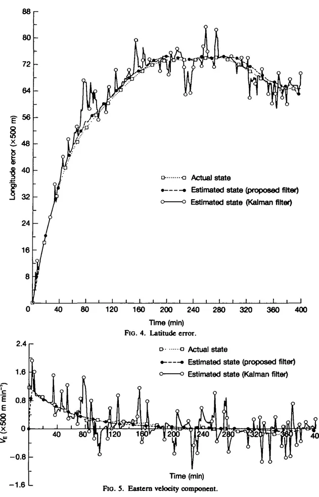
for / = 1, 2. From these results, it is clear that, whenever the proposed filter is used, the behaviour of the estimated state is very similar to that of the actual state and their values are fairly close (see Figs. 2-7). It is also clear from Fig. 7 that, whenever the Loran-C errors jump from one state to another, the proposed filter tends to follow these jumps with reasonable accuracy. On the other hand, the Kalman filter does not respond at all to these jumps. Indeed, from these results, it is clear that the response of the proposed filter to the rapid changes of the

88 80 72 64 48 40 32 24 16 2.4 r o -a Actual state

• - • Estimated state (proposed filter) o o Estimated state (Kaiman filter)

40 80 120 160 200 240 280 320 360 400

Time (min) FIG. 4. Latitude error.

D a Actual state

• - — • Estimated state (proposed filter) o o Estimated state (Kaiman filter)

400

- 1 . 6 L

Time (min) Fio. 5. Eastern velocity component.

400

- 1 . 6 L

24

12

Time(min) Fio. 6. Northern velocity component. - (a) Actual state

-24 L 24 12 £ 0 - 1 2 -24 L 12 -£ 0 12 -- 2 4 L

Estimated state (proposed fitter)

cant 40 -80 law \r\ou 120 1 1 1 Li i-l -1 1 J 160 200 240 Time (mln) 280 320 360 400

241- (b) Actual 3tate

12

-- 2 4 L

24 r Estimated state (proposed filter)

- 2 4 L

24 r Estimated state (Kalman fitter)

E 1 2 - 1 2 - 2 4 L -ft. _{I —. '— -— I — ' [ 1 U.} 40 80 120 160 200 240 Time (min) FIG. 7 (contd). 280 320 360 400

Loran-C error is much better than that of the Kalman filter, and hence one expects better estimates of position and velocity. Finally, it should be noted that similar results have been obtained for the case where an Omega receiver (which is modelled in a similar way to Loran-C) is used along with DR and Loran-C. 6. Conclusions

In this paper, we have considered the filtering problem for a class of jump processes with discrete observations. Under the assumption that the elements of the covariance matrices of state and observation noise are very small compared

2 9 2 T. E. DABBOUS, S. S. UM, AND N. U. AHMED

with the size of jump of the state process, we have obtained a recursive linear unbiased minimum variance filter. Using these filter equations, we have also studied the question of continuous dependence of the filter on system parameters. Finally, we have presented a numerical example, which is based on a navigation system, to illustrate the effectiveness of the proposed filter. From this example, we have seen that the estimated states computed via the proposed filter are closer to the actual states than those obtained by use of the Kalman filter. Further, we have also observed that the proposed filter is able to follow the rapid changes of the Loran-C error more closely than the Kalman filter, and hence better estimates for ship (or aircraft) position and velocity can be obtained.

REFERENCES

1. AHMED, N. U. 1988 Elements of Finite-Dimensional Systems and Control Theory. Harlow: Longman.

2. AHMED, N. U. 1988 Optimization and Identification of Systems Governed by Evolution Equations on Banach Space, Pitman Research Notes in Mathematical Sciences 184. Harlow: Longman.

3. DABBOUS, T. E., AHMED, N. U., MCMILLAN, J. C , & LIANG, D. F. 1988 Filtering of discontinuous processes arising in marine integrated navigation systems. IEEE Trans. Aerospace Electron. Syst. 24, 85-102.

4. AHMED, N. U., & DABBOUS, T. E. 1983 Modelling and on-line control and reliability dynamics of large scale interconnected power systems. Int. J. Syst. Set. 14, 1321-53. 5. AHMED, N. U., & DABBOUS, T. E. 1986 Nonlinear filtering of systems governed by

Ito differential equations with jump parameters. J. Math. Anal. Appl. 115, 76-92. 6. DABBOUS, T. E., & AHMED, N. U. 1981 Nonlinear filtering of diffusion processes with

discontinuous observations. J. Stochast. Anal. Appl. 2(4), 87-106.

7. KUSHNER, H. J. 1967 Dynamical equations for optimal nonlinear filtering. J. Diff. Eqn. 3, 179-190.

8. ZAKAI, M. 1969 On the optimal filtering of diffusion processes. Z. Wahrsch. Verw. Gtb. 11, 230-43.

9. AHMED, N. U., & DABBOUS, T. E. 1985 Study of discontinuous processes in Omega and Loran-C radio signals. Report submitted to Defence Research and Establishment Ottawa, Ottawa, Canada.

10. AHMED, N. U., & LIM, S. S. 1987 Continuation of the study of discontinuous processes in Omega and Loran-C radio signals. Report submitted to Defence Research and Establishment Ottawa, Ottawa, Canada.

11. JAZWINSKI, A. H. 1970 Stochastic Processes and Filtering Theory. London: Academic Press.

12. SKOROKHOD, A. V. 1965 Studies in The Theory of Random Processes. Reading, MA: Addison-Wesley.

13. BOEL, R., VARATYA, P., & WONG, E. 1975 Martingales on jump processes n . SI AM J. Control Optim. 13, 1022-60.

14. TAKEUCHI, Y., & AKASHI, H. 1981 Nonlinear filtering formulas for discrete time observations. SIAM J. Control Optim. 19, 244-61.