APPLYING AN OBJECT-BASED CLASSIFICATION APPROACH THROUGH A CELLULAR AUTOMATA-MARKOV METHOD IN LANDCOVER/LANDUSE CHANGE DETECTION
PROCEDURE "CASE OF THE URMIA LAKE”
1Ramiz MAMMADOV, 2Ali Akbar RASULY, 3Hanieh MOBASHER, 4Keyvan MOHAMADZADEH 1The Institute of Geography, National Academy of Sciences, University of Baku AZERBAIJAN
2Department of Environmental Sciences, Macquarie University, Sydney, AUSTRALIA 3University of Tabriz, Department of RS & GIS, Tabriz, Azerbaijan, IRAN
1[email protected], 2[email protected] 3[email protected],4[email protected]
(Geliş/Received: 08.11.2018; Kabul/Accepted in Revised Form: 06.12.2018)
ABSTRACT: The main aim of the present research was to reveal changes on Land-Cover/Land-Use
Changes (LC/LUC) patterns in the in the northern coast of the Urmia Lake by applying an object-based image analysis (OBIA) process. Accordingly, in the image process procedures stage, spatial changes on the Urmia Lake surfaces were carefully acquired from the Landsat imageries, since 1987 to 2016. Then, in the second stage, LC/LU change patterns have been precisely delineated, for the southern hillsides of the Misho Mountain. The resulting models showed an overall accuracy of nearly about 92.54% and a Kappa coefficient of 91% in the image classification procedures. In the final stage, by introducing a Cellular Automata-Markov (CA-Markov) method and setting a transition matrix, the spatial changes on the LC/LU patterns have been progressively simulated for the approaching years till year 2020 inside the study area. The final models illustrate a meaningful significant decrease in the Urmia Lake surface, accompanying by certain water volumes diminishing tendency, highlighting the fact that the amount of salty lands are meaningfully increasing. This harmful inclination has successively causes a critical diminishing on the vegetation’s types by emerging the most recent changes on LC/LU types accompanying by a critical hyper-saline condition mainly around the coastal parts of the Urmia Lake.
Implementations of the current significant changes strongly pointing up that the majority of local biotic and abiotic components are in imitate dangers with serious environmental negative observations. Such rapidly occurring revolutionized changes on LC/LU will impose various critical effects on the existing in danger ecosystems and vulnerable climatic sub-systems in immediate prospect.
Key Words: Landuse Changes, Object-Based Approach and CA-Markov Method, Urmia Lake
Urmiye Gölü Örneğinde Arazi/Arazi Değişimi Tespit Prosedüründe Hücresel Otomata Markov Yöntemi İle Nesne Tabanlı Sınıflandırma Yaklaşımının Uygulanması
ÖZ: Mevcut araştırmanın temel amacı, nesne tabanlı bir görüntü analizi (OBIA) işlemi uygulayarak
Urmiye Gölü'nün kuzey kıyılarındaki Arazi Örtüsü / Arazi Kullanım Değişiklikleri (LC / LUC) modellerinde değişiklikleri ortaya koymaktı. Buna bağlı olarak, görüntü işleme prosedürleri aşamasında, Urmiye Gölü yüzeylerindeki uzamsal değişiklikler, 1987'den 2016'ya kadar Landsat görüntülerinden dikkatlice alınmıştır. Ardından, ikinci aşamada, Misho Dağı'nın güney yamaçları için LC / LU değişim modelleri kesin olarak tanımlandı. Elde edilen modeller, görüntü sınıflandırma prosedürlerinde yaklaşık% 92,54 genel bir hassasiyet ve% 91'lik bir Kappa katsayısı gösterdi. Son aşamada, Hücresel Otomata-Markov (CA-Markov) yönteminin tanıtılması ve bir geçiş matrisinin ayarlanmasıyla, LC / LU
modellerinde uzamsal değişiklikler, çalışma alanı içinde 2020 yılına kadar yaklaşan yıllar boyunca aşamalı olarak simüle edilmiştir.
Nihai modeller, Urmia Gölü yüzeyinde, belirli su hacimlerinin eşlik ettiği ve azalan eğilimde anlamlı bir düşüş olduğunu göstermektedir, bu da tuzlu toprakların miktarının anlamlı şekilde arttığını vurgulamaktadır. Bu zararlı eğim, esas olarak Urmiye Gölü'nün kıyı bölgelerinde, kritik bir hiper-salin durumunun eşlik ettiği LC / LU tiplerinde en son değişikliklerin ortaya çıkmasıyla bitki örtüsünün tiplerinde kritik bir azalmaya neden olur. Mevcut önemli değişikliklerin uygulanması, yerel biyotik ve abiyotik bileşenlerin çoğunun ciddi çevresel olumsuz gözlemlerle taklit tehlikeler içinde olduğuna işaret etmektedir. LC / LU’ta bu tür hızlı bir şekilde meydana gelen devrim niteliğindeki değişiklikler, acil durumdaki tehlike ekosistemlerinde ve hassas iklimsel alt sistemlerde var olan çeşitli kritik etkiler yaratacaktır.
Anahtar kelimeler: Arazi Kullanım Değişiklikleri, Nesneye Dayalı Yaklaşım ve CA-Markov Yöntemi, Urmiye Gölü
INTRODUCTION
Land is one of the essential natural resources (Rahman et al., 2012). The unprecedented rate of land change has become a major concern around the world that’s why this issue has affected the environmental services and biodiversity at the global level. Both anthropogenic and natural forces are responsible for these changes in Earth’s surface. Anthropogenic forces such as urban expansion and the destruction of forests and meadows for economic purposes (development of agricultural land); and natural forces such as fire, flood and tsunami; have changed the type of land cover/use (LC/LU) all over the world (Keshtkar and Voigt, 2016). Monitoring and assessing LC/LU information is one of the most essential for managing natural resources and a variety of planning.
In recent decades, research has shown considerable progress towards assessing LUCC. Remote sensing technology is one of the suitable technologies for monitoring environmental and land cover/use changes, which has multi temporal, resolution and spectral capabilities (Rasuly et al., 2009). Landsat spectral data, which are free on the United States Geological Survey (USGS) website for downloading, have a remarkable temporal range of over 40 years and have great potential for LC/LU classification, change detection, and relevant analysis (Roy et al., 2014). A new classification method, object-based image analysis (OBIA), referred to as edge-detection, feature extraction, feature analysis or object-based remote sensing, appears to used best on satellite imagery (Blaschke, 2010). This form of feature extraction lets to use of additional variables such as shape, texture, and contextual relationships to classify image features.
In addition, geographic information systems (GIS) and remote sensing tools enable researchers to predict future LC/LU changes (Keshtkar and Voigt, 2016). In this research, we applied a cellular automata– Markov chain model (CA–Markov) to simulate future LC/LU changes. Both CA and the Markov chain model have great advantages in the study on LULC changes. The Markov model can quantitatively predict the dynamic changes of landscape patterns, but it is difficult to predict the spatial pattern of land use changes. In contrast the CA model with strong spatial computing can be used to simulate the spatial variation of the system effectively (Kamusoko et al., 2009).
The objectives of this study are (1) Object-based classification Landsat imageries, which were converted into TOA reflectance; (2) Analyzing LC/LU changes from 1987 to 2016; (3) Predict future LC/LU change in 2020 based on CA-Markov model. The Markov-CA model contributes to the understanding of LC/LU change in the northern coast of the Urmia Lake, which facilitates future planning.
MATERIALS AND METHODS Study Area and Materials
The study area is located between 38° 0′ 32″ and 38° 25′ 28″ latitude and between 44° 57′ 23″ and 46° 01′ 14″ longitude in north-west of Iran (the Southern hillsides of the Misho Mountain and the northern coast of the Urmia Lake. The total area covers about 2951 km2 (Figure 1). The elevation of the study area varies from approximately 3100 m to 1270 m above mean sea level.
Figure 1. Study area - location of Urmia Lake in the Northwest of Iran and Middle East
Misho Mountain is one of the most important animal husbandry and agricultural center in the East Azerbaijan province which separate Marand plain from Shabestar plain and Urmia Lake. Also, the Urmia Lake is as a second largest salty lake in the world. The Urmia Lake is located in the north-west of Iran; as a second largest salty lake in the world. The last decade droughts based on climate change episodes, water consumption in agricultural fields, artificial coastal changes (roads building operations) and importantly dam construction programs have simultaneously caused more evaporation of the lake water and thus considerable variations of water surface levels. Average salinity of the lake ranges between 220- 300 mg/lit depending upon temporal and spatial conditions. It is worth to identify that Urmia Lake is the 20th largest lake and the second hyper-saline lake in the world and its basin is covered about 3.15 percent of the whole country (Rasouli et al., 2016).
Data Analyzed
Landsat imageries with a 30 m spatial resolution (path/row 169/33) were the main data for this study. The earliest one was Landsat Thematic Mapper (TM) taken on June 1987. The images were obtained from United States Geological Survey (USGS) site. Based on accessible time intervals and the image quality, other Landsat (ETM+ and OLI) images were provided and have been taken on different image processing
procedures respectively. A 30 m Digital Elevation Model (DEM), based on Aster imagery, was also employed. Table 1 indicates all datasets which have been processed in current study.
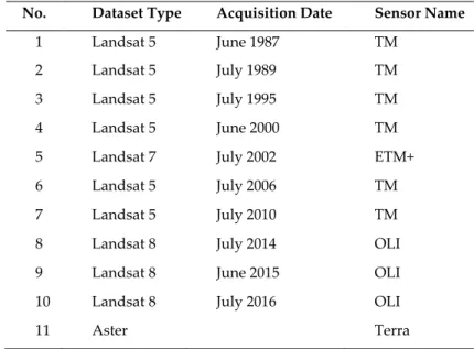
Table 1. Dataset summary
No. Dataset Type Acquisition Date Sensor Name
1 Landsat 5 June 1987 TM
2 Landsat 5 July 1989 TM
3 Landsat 5 July 1995 TM
4 Landsat 5 June 2000 TM
5 Landsat 7 July 2002 ETM+
6 Landsat 5 July 2006 TM
7 Landsat 5 July 2010 TM
8 Landsat 8 July 2014 OLI
9 Landsat 8 June 2015 OLI
10 Landsat 8 July 2016 OLI
11 Aster Terra
Methods Applied
The image processing was performed in four stages including pre-processing, object oriented classification, post processing and predicting a LULC for 2020.
Data pre-processing
In the pre-processing stage radiometric correction and atmospheric correction are prerequisite for generating high-quality scientific data (Chander et al., 2009), making it possible to discriminate between product artefacts and real changes in Earth processes (Justice et al., 2002) as well as accurately produce LULC maps and detect changes (Song et al., 2001). The radiometric conversion for The Landsat TM and ETM+ was performed in the software of Environment for Visualizing Images (ENVI, Version 5.3) by following the Equations (1) and (2), where the spectral radiance (𝑳𝝀) and the TOA reflectance (𝝆𝝀) were
obtained: 𝐿𝜆= ( 𝐿𝑚𝑎𝑥−𝐿𝑚𝑖𝑛 𝑄𝑐𝑎𝑙𝑚𝑎𝑥−𝑄𝑐𝑎𝑙𝑚𝑖𝑛) × (𝑄𝑐𝑎𝑙− 𝑄𝑐𝑎𝑙𝑚𝑖𝑛) + 𝐿𝑚𝑖𝑛 (1) 𝜌𝜆 = 𝜋×𝐿𝜆×𝑑2 𝐸𝑆𝑈𝑁𝜆×𝑐𝑜𝑠 𝜃𝑆 (2) 𝑑𝑟 = 1 + 0.033 𝑐𝑜𝑠 (𝐷𝑂𝑌 2𝜋 365) (3) where:
𝑳𝒎𝒂𝒙 = the spectral radiance scales to 𝑸𝒄𝒂𝒍𝒎𝒂𝒙 𝑳𝒎𝒊𝒏 = the spectral radiance scales to 𝑸𝒄𝒂𝒍𝒎𝒊𝒏
𝑸𝒄𝒂𝒍𝒎𝒂𝒙= the maximum quantized calibrated pixel value 𝑸𝒄𝒂𝒍𝒎𝒊𝒏= the minimum quantized calibrated pixel value 𝑸𝒄𝒂𝒍 = DN
𝒅 = the distance from the earth to the sun 𝑫𝑶𝒀 = Day of year
𝑬𝑺𝑼𝑵𝝀=mean solar exo-atmospheric irradiance 𝜽𝑺 = Solar zenith angle
In the case of the data from the Landsat 8, the radiometric conversion was performed by applying the equations (4) and (5): ρˊλ= Mρ× 𝑄cal+ Ap (4) 𝜌𝜆 = 𝜌ˊ𝜆 𝑠𝑖𝑛 𝜃𝑆𝐸 (5) where:
𝑴𝝆= Band-specific multiplicative rescaling factor
𝑨𝒑 =Band-specific additive rescaling factor
𝝆ˊ𝝀= TOA planetary reflectance, with correction for solar angle
𝜽𝑺𝑬 = the local sun elevation angle.
ENVI has a quick atmospheric correction module for retrieving spectral reflectance. This method can be very time-consuming; hence to reduce the time of image processing all data were subset with a vector file of study area.
Image processing
At the processing stage, we used object-based classification method based on a set of spectral, texture and contextual indicators. In general, this method aiming to relate geographic features with image objects can be divided into two main parts, namely segmentation and classification (Liu et al., 2008). This method uses geographic objects as basic units for LULC classification. We used eCognition Developer 9.0 to classification each date of imagery. The eCognition software provides a systematic approach and user-friendly interface that permits implementation of concepts developed in the past (Campbell and Wynne, 2011). Based on different standards such as quality of segmentation without considering classification accuracy, they found that eCognition segmentation was better than the alternatives, including ERDAS Imagine, for a variety of reasons including having different segmentation algorithms and classifiers (Meinel and Neubert, 2004). In software setting, the image classification is based on attributes of image objects rather than on the attributes of individual pixels. Therefore, Object-oriented classifier found to deliver results noticeably better than conventional methods. It leads to better semantic differentiation and higher classification accuracy (Rasouli et al., 2016). The quality of classification is directly affected by segmentation quality. Image segmentation means the partitioning of an image into meaningful regions based on homogeneity or heterogeneity criteria, respectively (Neubert et al., 2006). This research used a multi-resolution segmentation approach, a bottom- up homogenous region aggregation technique based on certain criteria (e.g., scale, shape, and compactness criteria). The scale parameter determines the size of objects (Benz et al., 2004). All non-thermal bands of the Landsat images (six bands) and DEM were used for image segmentation. The appropriate segmentation scale and the parameters associated are indicated in Table 2.
Table 2. Multi-resolution segmentation parameters
Scale Shape Compactness Band Weights
25 0.2 0.5 Blue (1), Green (1), Red (1), NIR (1), SWIR1 (1), SWIR2 (1), DEM (1)
At the classification stage we used the assign class algorithm to classify the image objects into 7 classes that Urmia Lake, salty area and agricultural area were our three main LULC by equations 6, 7, 8, 9, 10 and11).
𝑁𝐷𝑉𝐼 1 =𝑁𝐼𝑅−𝑅𝑒𝑑 𝑁𝐼𝑅+𝑅𝑒𝑑 (6) 𝑁𝐷𝑊𝐼 2 =𝐺𝑟𝑒𝑒𝑛−𝑁𝐼𝑅 𝐺𝑟𝑒𝑒𝑛+𝑁𝐼𝑅 (7) 𝑆𝐼9 3 =𝐵𝑙𝑢𝑒∗𝑅𝑒𝑑 𝐺𝑟𝑒𝑒𝑛 (8) 𝑆𝐼10 4 =𝐵𝑙𝑢𝑒 𝑅𝑒𝑑 (9) 𝑁𝐷𝑆𝐼 5 =𝑅𝑒𝑑−𝑁𝐼𝑅 𝑅𝑒𝑑+𝑁𝐼𝑅 (10) 𝑩𝑺𝑰 6 =(𝑺𝑾𝑰𝑹𝟏+𝑹𝒆𝒅)−(𝑵𝑰𝑹+𝑩𝒍𝒖𝒆) (𝑺𝑾𝑰𝑹𝟏+𝑹𝒆𝒅)+(𝑵𝑰𝑹+𝑩𝒍𝒖𝒆) (11)
A classification is not complete until its accuracy is assessed (Lillesand et al., 2014). Accuracy assessment of classification maps was achieved using a random sampling method. After land-cover classification, a minimum of about 50 sample points were randomly selected for the evaluation of classification accuracy for six land-cover classes. Accuracy assessment was based on the calculation of the overall accuracy and kappa coefficient.
LC/LU change analysis
Post-classification analysis allows us to know the quantity, location and nature of LULC changes by comparing two classified maps; in such a way, a “from- to” matrix of changes was generated Sanchez-Reyes et al. (2017) using the Cross tabulation module of IDRISI Selva 17.0. The ten images classified by object oriented were pairwise compared to detect patterns of change between 1987–1989, 1989–1995, 1995–2000, 2000–2002, 2002- 2006, 2006- 2010, 2010- 2014, 2014-2015 and 2015-2016 .
Markov Chain analysis
This kind of predictive LULC change modeling is appropriate when the past trend of LULC changing pattern is known (Eastman, 2009). A Markov chain is a stochastic process (based on probabilities) with discrete state space and discrete or continuous parameter space (Balzter, 2000). In this random process, the state of a system s at time (t+1) depends only on the state of the system at time t, not on the previous states. The Markov model not only explains the quantification of conversion states between the LULC types, but can also reveal the transfer rate among different LULC types. It is commonly used in the prediction of geographical characteristics with no after-effect event which has now become an important predicting method in geographic research (Li et al., 2015). Based on the conditional probability formula, the prediction of LULC changes is calculated by the equation 12:
𝑆(𝑡+1) = 𝑃(𝑖𝑗)× 𝑆(𝑡) (12)
Where 𝑺(𝒕), 𝑺(𝒕+𝟏) is the system status at the time of (t) or (t + 1); 𝑷(𝒊𝒋) is the transition probability matrix
1 Normalized Difference Vegetation Index 2 Normalized Difference Water Index 3 Salinity Index 9
4 Salinity Index 10
5 Normalized Difference Salt Index 6 Bare Soil Index
in a state which is calculated by equations 13 and 14 (Xiyong et al., 2004): 𝑃𝑖𝑗= [ 𝑃11 𝑃12 … 𝑃1n 𝑝21 𝑝22 … 𝑝2n ⋮ ⋮ ⋮ ⋮ 𝑝𝑛1 𝑝𝑛2 … 𝑝𝑛𝑛 ] (13) (0 ≤ 𝑃𝑖𝑗≤ 1 and ∑𝑁 𝑃𝑖𝑗= 1, 𝑗=1 (i, j = 1,2 3, … , n)) (14)
According to the matrix of the initial 𝑺(𝟎) and the transition probability of the nth stage 𝑷(𝒏), the LULC
distribution in the northern coast of the Urmia Lake in the future can be calculated by using a computer simulation. The Markov simulation model 𝑺(𝟎) is calculated by equation 15:
𝑺(𝒏)= 𝑺(𝒏−𝟏)× 𝑷(𝟏)= 𝑺
(𝟎)× 𝑷(𝒏) (15)
Multi Criteria Evaluation (MCE)
Multi-Criteria Evaluation process (MCE) involves criteria of varying importance in accordance to decision makers and information about the relative importance of the criteria (Behera et al., 2012). Factors used in MCE account for suitability, accessibility, and neighbourhood effects. This suitability maps determine which pixels will change as per the highest suitability of each LULC type.
CA model
Cellular Automata is a simulation model where the space and time are discrete variables and interactions assigned are local variables. In a CA model, the transition of a cell from one land-cover to another depends on the state of the neighbourhood cells. This is based on the idea that a cell will have a higher probability to change to land-cover class ‘A’ than to a land-cover class ‘B’ if the cell is in closer proximity to land-cover class ‘A’. Thus the CA model not only uses the information of the previous state of a land-cover as done by a Markov model but also uses the state of neighbourhood cells for its transition rules (Adhikari and Southworth, 2012).
Markov – CA model
The Markov model can quantitatively predict the dynamic changes of landscape pattern, while it is not good at dealing with the spatial pattern of landscape change. On the other hand, Cellular Automata (CA) has the ability to predict any transition among any number of categories (Pontius & Malanson, 2005).Combining the advantages of Cellular Automata theory and the space layout forecast of Markov theory, CA-Markov model performs better in modelling LULC change in both time and spatial dimension. At present, IDRISI software is one of the best platforms to conduct CA-Markov model, which is developed by Clark Labs in the U.S.
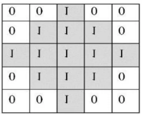
In this study we used the CA–Markov model to simulate LULC. Three datasets, (1) LULC base map in 2010, (2), the 2010 land suitability maps which created by using MCE (Multi-Criteria Evaluation) model and (3), transition probability matrix from 2006 to 2010 are integrated using CA neighbourhood to simulate land use map in 2016. The standard 5×5 contiguity filter is used as the neighbourhood definition in this study. That is, each cellular center is surrounded by a matrix space which is composed by 5×5 cellular to impact the cellular changes significantly. The filter used analysis is based on:
Figure 2. Filter configuration used in CA Markov Model validation
In order to ensure that the model is reliable in predicting an LC/LU for a specific project year, it must be validated using existing datasets (Hadi et al., 2014). Now the aim is to select the most appropriate model. The traditional way of validating a model or comparing two maps, using Kappa statistics, is now out-of-date (Ahmed and Ahmed, 2012). A method of comparing three maps (a reference map of time 1, a reference map of time 2 and a simulation map of time 2) has been implemented for model validation (Pontius et al., 2011). The confirm module in IDRISI Selva was used for validating the model by producing After converting Landsat radiance values to reflectance and eliminating the negative effects of molecular scattering and aerosols the quality of the image was improved. As we have mentioned we applied an object- oriented image analysis of eCognition software for the classification LC/LU on Landsat images between 1987 and 2016. Object-oriented image analysis requires the several parameters: standard, K-location, and K-no which are used to identify the accuracy of the model. The predictive power of the model is considered strong when around 80% accuracy is achieved (Eastman, 2009). At the end, following the same process, the LC/LU for the year 2020 was projected with the CA–Markov model using the transition probabilities from 2010 to 2016 and the LC/LU base map from the year 2016.
RESULTS
Converting Landsat Radiance Values to Reflectance
After converting Landsat radiance values to reflectance and eliminating the negative effects of molecular scattering and aerosols the quality of the image was improved.
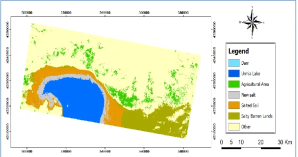
Land use/cover classification
As we have mentioned we applied an object-oriented image analysis of eCognition software for the classification LULC on Landsat images between 1987 and 2016. Object-oriented image analysis requires the creation of objects or separated regions in an image. After conducting the Multi Resolution Segmentation process, we developed the rule sets for classifying each test area. Then, the threshold values were obtained (Table 3). Figure (3) indicates the LC/LU map of the study area. The results from the classification were shown in Table 4, indicating the total area and percentages of LC/LU classes.
Table 3. Threshold values for each rule
LC/LU Classes Threshold Conditions
Urmia Lake NDWI > −0.138
NDSI > −0.096 New Salt S𝐼9 > 750 BSI < 0.17
Salted Soil S𝐼10 > 0.48
Salty barren lands NDS𝐼 > −0.32
Br𝑖𝑔ℎtness > 2700 Vegetation (Agricultural and Garden Lands) NDVI > 0.35 Me𝑎n DEM ≤ 1735
Dams and Agricultural ponds
NDWI > −0.138 Mean DEM < 1300
Table 4. Area and percentage of LC/LU classes Year LC/LU 1987 1989 1995 2000 2002 2006 2010 2014 2015 2016 Dams and Agricultural ponds Area 0.0044 0.028 0.081 0.104 0.094 0.112 0.186 0.25 0.418 0.332 percentages 0.001 0.001 0.003 0.04 0.003 0.004 0.006 0.008 0.014 0.011 Urmia Lake Area 742.954 761.564 813.567 721.976 670.681 642.403 515.919 290.438 306.442 378.678 percentages 25.182 25.81 27.58 24.47 22.73 21.77 17.49 9.84 10.39 12.83 Agricultural Area Area 251.813 169.811 239.697 233.447 212.806 197.134 157.08 190.877 209.867 172.872 percentages 8.535 5.76 8.12 7.91 7.21 6.68 5.32 6.47 7.11 5.86 New Salt Area 19.147 8.609 5.1589 10.915 20.54 31.641 56.498 144.374 133.658 117.779 percentages 0.649 0.29 0.17 0.37 0.7 1.07 1.91 4.89 4.53 3.99 Salted Soil Area 19.088 26.941 3.593 58.754 110.003 129.647 165.063 303.208 298.631 240.158 percentages 0.647 0.91 0.12 1.99 3.73 4.39 5.59 10.28 10.12 8.14 Salty Barren Lands Area 291.816 227.635 230.895 279.207 216.221 254.975 331.64 283.545 300.067 332.906 percentages 9.891 7.72 7.83 9.46 7.33 8.64 11.24 9.61 10.17 11.28 Other Lands Area 1625.497 1755.772 1657.376 1645.957 1720.016 1694.447 1723.97 1737.666 1701.275 1707.634 percentages 55.095 59.51 56.18 55.79 58.3 57.43 58.43 58.9 57.66 57.88 Total Area 2950.4 2950.4 2950.4 2950.4 2950.4 2950.4 2950.4 2950.4 2950.4 2950.4
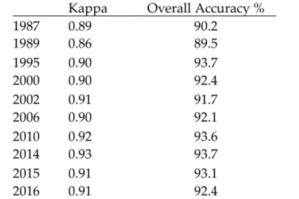
The accuracy of the classified image was then assessed by using randomly selected around 50 points. Table 5 informs the results of the overall accuracy and kappa. This accuracy assessment shows that the classification is stable.
Table 5. The classification accuracy values and Kappa coefficients
Year
Kappa Overall Accuracy %
1987 0.89 90.2 1989 0.86 89.5 1995 0.90 93.7 2000 0.90 92.4 2002 0.91 91.7 2006 0.90 92.1 2010 0.92 93.6 2014 0.93 93.7 2015 0.91 93.1 2016 0.91 92.4
LULC Changes (Directions and Trends of the Urmia Lake Growth Model)
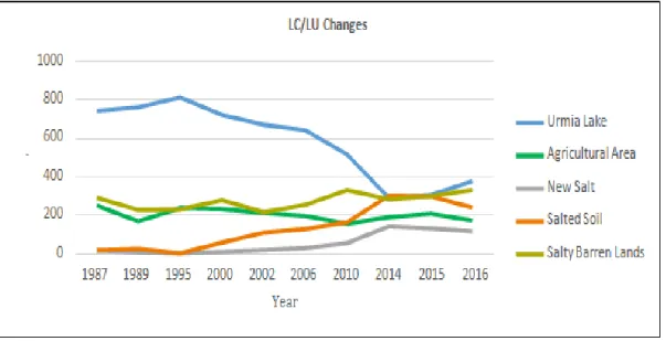
The overall classification accuracy for the extracted LC/LU maps in Table 3 indicate the suitability of the classified remote sensing images for effective LC/LU change analysis. A cross tabulation process was applied to identify the major changes between two LC/LU maps of the specified time periods. Trend of LC/LU change maps in each class from the nine periods are displayed in Figure 4.
Figure 4. LC/LU changes (km2)
There was a lot of fluctuation in the amounts of LC/LU changes. Spatial analysis of the LC/LU changes illustrates evidently that the conversions between Urmia Lake and salt was the most distinctive change of the study period. According to the graph, from 1987 to 2016, there was sharp fall in the Urmia Lake surfaces and a gradual decrease in agricultural lands. However, there is a slight increase in salty lands.
CA-Markov Model Transition Matrix
The LC/LU was projected using Markov’s transition probability matrix (Tables 6 and 7) to show how each land type was projected to change. The diagonal of the transition probability represents the self-replacement probabilities, that is, the probability of a salt cover class remaining the same, whereas the off-diagonal values indicate the probability of a change occurring from one salt cover class to another. The LC/LU map in 2006 and 2010 were operated by the Markov chain model in order to identify the probability of changing and transition areas.
Such probability transition values were applied to predict the LC/LU for the year 2016 with a CA_Markov model.
Table 6. Transition probability matrix, calculated based on LC/LU maps of 2006-2010 LC/LU Dams and Agricultural ponds Urmia Lake Agricultural Area New Salt Salted Soil Salty Barren Lands Other Lands Dams and Agricultural ponds 0.579 0 0.0013 0 0 0.0022 0.4175 Urmia Lake 0 0.7177 0 0.079 0.1978 0.0041 0.0014 Agricultural Area 0 0 0.5558 0 0.0001 0.0027 0.4415 New Salt 0 0.0017 0.0006 0.0004 0.6603 0.3151 0.0218 Salted Soil 0 0.0005 0.0014 0.0001 0.3307 0.5870 0.0803
Salty Barren Lands 0 0 0.0005 0 0.0015 0.8783 0.1197
Table 7. Transition probability matrix, calculated based on LC/LU maps of 2010-2016 LC/LU Dams and Agricultural ponds Urmia Lake Agricultural Area New Salt Salted Soil Salty Barren Lands Other Lands Dams and Agricultural ponds 0.7844 0 0 0 0 0.0701 0.1455 Urmia Lake 0 0.8104 0 0.1888 0 0.0007 0.0001 Agricultural Area 0 0 0.8492 0 0 0 0.1507 New Salt 0 0.0002 0 0.1771 0.8227 0 0 Salted Soil 0 0.0005 0 0.0154 0.9621 0.0207 0.0013
Salty Barren Lands 0 0 0 0 0.0085 0.9419 0.0495
Other Lands 0.0001 0 0.0203 0 0.0003 0.0096 0.9698
Model Validation
For the model validation, we compared the simulated map of 2016 with the actual LC/LU map. The K-standard, K- no, and K-location indicators resulted in measures of 89.4%, 91.26% and 94.02%, respectively. Visual comparison also shows great similarity between the actual and simulated maps for the year 2016 (Figure 5).
The Kappa statistics value indicates that the CA–Markov model was effective in simulating LC/LU change in 2016. Therefore, the Markov–CA model can be used to predicting the spatial distribution of LC/LU in the future with the assumption that an unvarying rate of change will occur in the future.
Figure 5. LC/LU map for year 2016: (a) actual map (b), simulated map Prediction of LC/LU changes for 2020
LC/LU map for the year 2020 were predicted (Figure 6). A Comparison of LC/LU maps for 2016 and 2020 shows that the extent of Urmia Lake in our study area and new salt will decrease from 378.7 km2 to 307.023 km2 and from 117.779 km2 to 96.0596 km2, respectively. As well the results show the salted soil, salty barren lands and agricultural areas will increase by 331.227 km2, 335.246 Km2 and 181.426 km2, respectively.
Figure 6. Predicted LC/LU map for year 2020 CONCLUDING REMARKS
The assessment of LC/LU changes and predicting future are crucial information for planners and organizations to allocate important infrastructures and land management in response to the diverse requirements of the people in this region. In this context, to accommodate this need, satellite images, objects-based classification and a combination of Markov chain analysis and CA were used.
The main advantage of OBIA is that it represents the classification units as real world objects on the ground, thereby reduces the within class variability. In addition, the CA–Markov land use simulation model has an important contribution to land use modeling.
In the present study, we were able to depict the relationship among LC/LU types in different time periods. A change survey of the study area revealed that water surface and the amount of salty lands are changing sharply. Thus it is urgent to strengthen the protection of arable land and water and prevent acts of indiscriminate use of cultivated land in order to promote land protection and rational use of land.
Reducing the surface of Lake Urmia and, as a result, increasing the salty lands around the lake, as well as reducing the agricultural area in the Misho Mountain, has increased the use of inhabitants from underground water, which is a reason to reduce the input water into the lake. Hence, by modifying the irrigation methods or choosing corps that have little water requirement, it is possible to improve the lake situation and increase its level.
Some recommendations are provided. First, Landsat data is not mandatory, any other type of image can be useful, and a higher resolution such as Spot imageries will greatly improve the results obtained. Second, it is suggested that data belong to similar dates in order to avoid seasonality, since an erroneous LC/LU classification could affect the succession analysis.
REFERENCES:
Adhikari, S., Southworth, J. Simulating forest cover changes of Bannerghatta National Park based on a CA-Markov model: a remote sensing approach. Remote Sensing, 2012 4(10), 3215-3243.
Ahmed, B., Ahmed, R. Modeling urban land cover growth dynamics using multi‑ temporal satellite images: a case study of Dhaka, Bangladesh. ISPRS International Journal of Geo-Information, 2012. 1 (1), 3-31.
Balzter, H., Markov chain models for vegetation dynamics. Ecological Modelling, 2000.126 (2-3), 139-154. Behera, D. M., Borate, S. N., Panda, S. N., Behera, P. R., Roy, P. S. Modelling and analyzing the watershed dynamics using Cellular Automata (CA)–Markov model–A geo-information based approach. Journal of earth system science, 2012. 121 (4), 1011-1024.
Benz, U. C., Hofmann, P., Willhauck, G., Lingenfelder, I., Heynen, M. Multi-resolution,object-oriented fuzzy analysis of remote sensing data for GIS-ready information. ISPRS Journal of Photogrammetry and Remote Sensing, 2004,58 (3-4), 239-258.
Blaschke, T. Object based image analysis for remote sensing. ISPRS Journal of Photogrammetry and Remote Sensing, 2010. 65 (1), 2-16.
Campbell, J. B., Wynne, R. H. Introduction to remote sensing (Vol. 5): Guilford Press: New York, NY, USA. 2011.
Chander, G., Markham, B. L., Helder, D. L. Summary of current radiometric calibration coefficients for Landsat MSS, TM, ETM+, and EO-1 ALI sensors. Remote sensing of environment, 2009. 113 (5), 893-903.
Eastman, J. R. IDRISI Taiga guide to GIS and image processing. Clark Labs Clark University, Worcester, MA. 2009.
Hadi, S. J., Shafri, H. Z., Mahir, M. D. Modelling LULC for the period 2010-2030 using GIS and Remote sensing: a case study of Tikrit, Iraq. Paper presented at the IOP conference series: earth and environmental science. 2014.
Justice, C., Townshend, J., Vermote, E., Masuoka, E., Wolfe, R., Saleous, N., Morisette, J. An overview of MODIS Land data processing and product status. Remote sensing of environment, 2002. 83 (1-2), 3-15. Kamusoko, C., Aniya, M., Adi, B., Manjoro, M. Rural sustainability under threat in Zimbabwe–simulation of future land use/cover changes in the Bindura district based on the Markov-cellular automata model. Applied Geography, 2009,29 (3), 435-447.
Keshtkar, H., Voigt, W. A spatiotemporal analysis of landscape change using an integrated Markov chain and cellular automata models. Modeling Earth Systems and Environment, 2016. 2 (1), 10.
Li, S., Jin, B., Wei, X., Jiang, Y., Wang, J. Using CA-Markov model to model the spatiotemporal change of land use/cover in Fuxian Lake for decision support. ISPRS Annals of the Photogrammetry, Remote Sensing and Spatial Information Sciences, 2015. 2 (4), 163.
Lillesand, T., Kiefer, R. W., Chipman, J. (2014). Remote sensing and image interpretation: John Wiley & Sons.
Liu, Y., Guo, Q., Kelly, M. A framework of region-based spatial relations for non- overlapping features and its application in object based image analysis. ISPRS Journal of Photogrammetry and Remote Sensing, 2008. 63 (4), 461-475.
Meinel, G., Neubert, M. A comparison of segmentation programs for high resolution remote sensing data. International Archives of Photogrammetry and Remote Sensing, 2004. 35 (Part B), 1097-1105. Neubert, M., Herold, H., Meinel, G. Evaluation of remote sensing image segmentation quality– further results and concepts. International Archives of Photogrammetry, Remote Sensing and Spatial Information Sciences, 2006.36 (4/C42).
Pontius, G. R., Malanson, J. Comparison of the structure and accuracy of two land change models. International Journal of Geographical Information Science, 2005. 19 (2), 243-265.
Pontius Jr, R. G., Peethambaram, S., Castella, J.-C. Comparison of three maps at multiple resolutions: a case study of land change simulation in Cho Don District, Vietnam. Annals of the Association of American Geographers, 2011. 101 (1), 45-62.
Rahman, A., Kumar, S., Fazal, S., Siddiqui, M. A. Assessment of land use/land cover change in the North-West District of Delhi using remote sensing and GIS techniques. Journal of the Indian Society of Remote Sensing, 2012. 40 (4), 689-697.
Rasuly, A. A., Mahdian, M. Moharrami. M. and Derrafshi, A. Signifying of the Urmia Lake Landuse Changes By Object-Oriented Image Processing Techniques. 2016.
Rasuly, A. A. Principle of applied remote sensing: image processing: Press Office: University of Tabriz, Tabriz, Iran. 2009.
Roy, D. P., Wulder, M., Loveland, T. R.,Woodcock, C., Allen, R., Anderson, M., Kennedy, R. Landsat-8: Science and product vision for terrestrial global change research. Remote sensing of environment, 2014. 145, 154-172.
Sánchez-Reyes, U. J., Niño-Maldonado, S., Barrientos-Lozano, L., Treviño-Carreón, J. Assessment of land use-cover changes and successional stages of vegetation in the natural protected area Altas Cumbres, Northeastern Mexico, using Landsat satellite imagery. Remote Sensing, 2017. 9 (7), 712.
Song, C., Woodcock, C. E., Seto, K. C., Lenney, M. P., Macomber, S. A. Classification and change detection using Landsat TM data: when and how to correct atmospheric effects? Remote sensing of environment, 2001. 75 (2), 230-244.