Recovery of 3-D objects with multiple curved surfaces from 2-D contours

(1)

E L S E V I E R Artificial Intelligence 67 (1994) 1-28

Artificial

Intelligence

Recovery of 3-D objects with multiple curved

surfaces from 2-D contours*

F a t i h U l u p i n a r * *

Department of Computer and Information Sciences, Faculty of Engineering, Bilkent University, Ankara, Turkey

R a m a k a n t N e v a t i a

Institute for Robotics and Intelligent Systems, School of Engineering, University of Southern California, Los Angeles, CA 90089-0273, USA

Received November 1991; revised December 1992

Abstract

Inference of 3-D shape from 2-D contours in a single image is an important problem in machine vision. Often, techniques to solve this problem examine each surface in the scene separately whereas our perception of their shapes clearly depends on the interplay between them as well. In this paper, we describe a technique that attempts to recover the shapes of all the surfaces of an object simultaneously, though it is limited to objects made of zero-Gaussian curvature surfaces. Our technique is based on an analysis of three kinds of symmetries defined in the paper and the constraints that derive from them, and from other boundaries. This technique uses some of the constraints developed in an earlier paper that was limited to examining a zero-Gaussian curvature surface cut by parallel planes. This restriction has been removed here and the constraints have been reformulated to allow integration of constraints from all the neighboring surfaces. Results on some complex examples are shown.

1. Introduction

O n e o f the basic goals o f mid-level vision is to r e c o v e r the local o r i e n t a t i o n s o f the surfaces o f the objects in a scene. O f the m a n y cues available to aid in this * This research was supported by the Advanced Research Projects Agency of the Department of Defense and was monitored by the Air Force Office of Scientific Research under Contract No. F49620-90-C-0078. The United States Government is authorized to reproduce and distribute reprints for governmental purposes notwithstanding any copyright notation hereon.

** Corresponding author. Present address: F. U1upmar, ACSC, 3000 S. Robertson Bl., Suite 400, Los Angeles, CA 90034, USA. E-mail: ulupinar@iris.usc.edu.

(2)

2 F. Uluptnar, R. Nevatia/Artificial Intelligence 67 (1994) 1-28

\

(~/ (bt

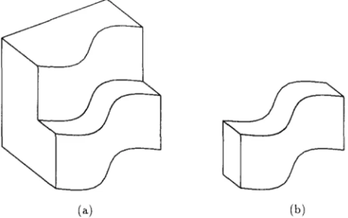
Fig. 1. (a) An object consisting of multiple planar and curved surfaces, and (b) the front part of the object in isolation.

process, we believe that shape of the 2-D contour itself is the most important and robust one. Of course, inferring shape from contour is highly ambiguous and cannot be done without making some assumptions. The goal in shape from contour methods is to minimize the number of needed assumptions and to achieve results consistent with human perception. For shape from contour analysis, the only ground truth is really in human perception, for even if the given contour was obtained by a real object, it

could

have been also obtained by any number of other objects as well.

Early work on inferring 3-D structure from a 2-D shape was focused on analysis of line drawings of polyhedra [3,6-9]. In the 80s, several techniques for non-polyhedral shapes were proposed (e.g. [1,2,5,10,11,13,18,19]). One characteristic of most of these methods is that they examine only a single surface in the scene at a time whereas our perception of a surface can be strongly influenced by our perception of the entire object.

In earlier papers, we have examined the recovery of 3-D surface shape of a variety of curved surfaces cut by planes [ 14,15,17 ] ). Our techniques rely on observed symmetries in the image and the analysis depends on the interplay between constraints imposed by the curved surface and the planes cutting it. We showed successful shape recovery for the following kinds of surfaces: zero- Gaussian curvature surfaces [ 14 ], surfaces of straight homogeneous generalized cylinders [15] and surfaces of planar, right, constant cross-section generalized cylinders [ 17 ].

Complex objects, however, are composed of a number of curved surfaces and planar patches. Our perception of each of these surfaces is affected by the presence of the others. For example consider the object in Fig. 1 (a) which appears to be a composite of two objects, one in front of the other. If the front object is viewed in isolation as in Fig. 1 (b), the interpretation for its top surface is ambiguous (it may be planar or not). However, in the context of the whole object (a), this ambiguity disappears (the said surface must be planar). This is an example of how a remote surface changes the perception of some

(3)

F. Ulupmar, R. Nevatia /Artificial Intelligence 67 (1994) 1-28 3

Fig. 2. Three cylinders intersected such that the middle cylinder has no planar cross-section. The perception of the middle cylinder, as being a circular cylinder, is much weaker compared to the side cylinders.

other surface drastically. In general, even if the perception of a surface may not be affected by the neighboring surfaces this drastically, its perception would still be affected by small amounts to make the whole object more consistent

(surfaces obeying inter-surface constraints).

This paper explores 3-D surface inference by including interplay between many surfaces that may comprise a complex object. Our technique is limited to a combination of zero-Gaussian curvature (ZGC) surfaces and planar surfaces, such that the intersection curves are planar. We can actually test the planarity of an intersection curve by using symmetries, since the symmetries presented in this paper only exist when the intersection curves are planar, except for very specific intersections violating the generality assumptions. We also conjecture that the shape information from contours degrades if the intersection of the surface produces non-planar curves. Fig. 2 shows an example.

Our method uses constraints similar to those used in our earlier work on shape from contour for ZGCs [14]. The previous work, however, was limited to analysis of a ZGC surface cut by two parallel planes. In this paper, we first develop techniques that allow analysis of a ZGC surface cut by non-parallel planes and then show how multiple ZGC surface shapes can be recovered simultaneously while influencing each other. To accomplish this, we have found it more convenient to change some of the representations used in our earlier work as well as to device an additional form of symmetry.

In Section 2 we define three kinds of symmetries and discuss the occurrence of these symmetries in the context of planar and ZGC surfaces. In Section 3 we discuss the constraint equations that are used in the shape recovery. In Section 4 the representation of the surfaces and single-surface recovery is discussed. In Section 5 combined shape recovery of multiple surfaces is discussed in detail. In Section 6 we discuss an implementation of the shape recovery algorithms and present some results.

Our method assumes that clean, closed boundaries are given (or can be extracted from the real image). We do not address the issue of separating object

(4)

F. Ulupmar, R. Nevatia /Artificial Intelligence 67 (1994) 1-28

boundaries from surface markings, or other perceptual grouping operations here, though we believe that constraints required for shape inference by our methods will aid in the perceptual organization process itself. Such research is being currently pursued in our laboratory separately.

We assume orthographic projection throughout the paper unless specifically mentioned otherwise. (In a separate paper, we have shown how many of the constraints for orthographic projection can be transformed to the case of perspective projection [ 16 ]. )

In this paper we will use gradient space to represent the orientation of surfaces (given by their normals). To review, the normal, N, of a plane ax + by + c z + d = 0 is given by the vector N = (a,b,c). This can be rewritten as (p, q, 1 ), where p = a/c and q = b/c (Note that this excludes cases where c = 0, however, such planes are parallel to the line of sight and are not imaged as planes under orthographic projection anyway.) (p, q) can be thought of as defining a two-dimensional space, called the gradient space, such that every point in this space corresponds to the normal of a plane in 3-D.

2. Surfaces and symmetries

In this paper we concentrate on shape from contour for objects composed of planar and zero-Gaussian curvature surfaces. A zero-Gaussian curvature (ZGC) surface is one where the Gaussian curvature (the product o f the max- i m u m and m i n i m u m principal curvatures) of the surface is zero everywhere. Cylinders and cones are examples of a Z G C surface. These surfaces are also called developable surfaces since they can be generated from a piece of paper by rolling a n d / o r bending without cutting. We feel that ZGC surfaces comprise

a large and useful class and that they represent a natural step up in complexity from the study o f planar surfaces that have dominated previous work in the field. Lines o f m i n i m u m curvature for a ZGC surface, also called rulings, are straight, i.e., it is possible to embed straight lines on a ZGC surface along these rulings.

2.1. Symmetries

We define three types o f symmetries that we call parallel symmetry, fine- convergent symmetry and skew symmetry. We show when such symmetries can be expected to occur and how they can be used to infer qualitative shape properties.

For curves to be symmetric, certain point-wise correspondences between two curves must exist. We will call the lines joining the corresponding points on the curves the lines of symmetry, the locus of the mid-points o f these lines the axis of symmetry, and the curves forming the symmetry the curves of symmetry.

(5)

F. Ulupmar, R. Nevatia /Artificial Intelligence 67 (1994) 1-28 i I ~ I • , I I I I ~ I ' . I I ! l t l ~ ,,~ I ". I I I . , . I I ~ ." / I I I ' | I ~, I . . ! I I I I . . " ~ / "..1 I I " . I I • I / " . . I V £ / ) " " I "" l ~ / , " ' . . ¢ . " l / (a) (b)

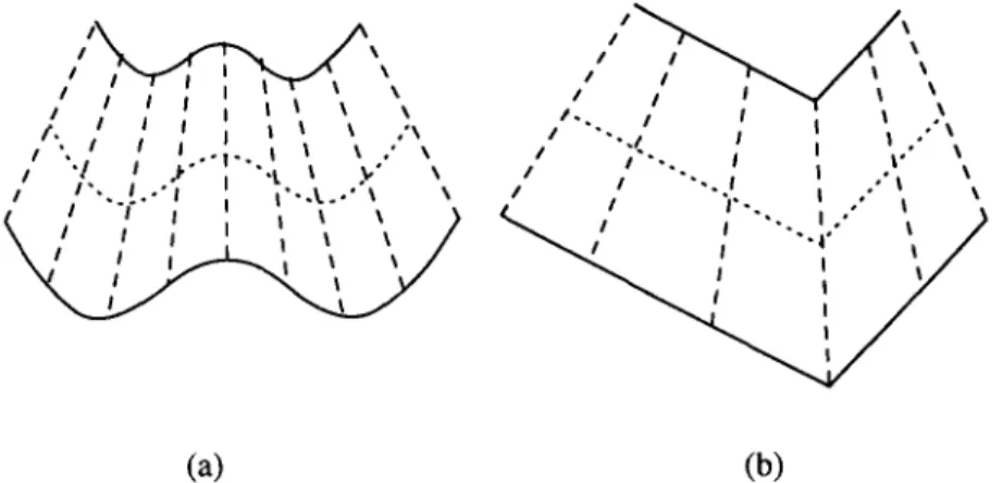
Fig. 3. Examples of (a) parallel symmetry with curved contours, and (b) parallel symmetry with straight contours. The dotted curves are axes of symmetry and the dashed lines are lines of symmetry.

2.1.1. Parallel symmetry

Consider two curves Xi(s) = ( x i ( s ) , y i ( s ) ) , for i = 1,2, parameterized by arc length s. Let T/(s) = (x~ (s), y~ (s)) be the unit tangent of the curves. Then, X1 (s) and X2(s) are said to be parallel symmetric if there exists a correspondence function f (s) between them such that Tl (s) = T2 ( f (s)) for all values of s for which X1 and X2 are defined and f (s) is a continuous monotonic function. A useful special case is when f (s) is restricted to be a linear function. In that case, the symmetry condition becomes: T1 (s) -- T2(as + b), where a and b are constant (a may be thought of as a scale parameter). Parallel symmetry with linear correspondence is found in cylindrical and conic surfaces (subsets of ZGC surfaces). In the context of ZGC surfaces parallel symmetry is obtained when ZGC surfaces are intersected by parallel planes [ 14]. Some examples are given in Fig. 3.

2.1.2. Line-convergent symmetry

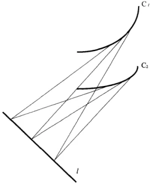
Two image curves

C1

and Cz are line-convergent symmetric if the tangents of C1 and C2, at the corresponding points, intersect along a line, say l, on the image plane. This is shown in Fig. 4. Parallel symmetry may be thought of as a limiting case of line-convergent symmetry where the line of intersection is at infinity. We show later, in Section 2.2, that this symmetry is found in curves obtained by cutting a ZGC surface with two non-parallel planes. A parallel symmetry also turns into line-convergent symmetry under perspective projection [ 16 ]. It is also present for limbs of straight homogeneous generalized cylinders [ 15 ].

2.1.3. Skew symmetry

In this symmetry, the point-wise correspondence should be such that the axis of the symmetry is straight, and the lines of symmetry are at a constant

(6)

F. Uluptnar, R. Nevath2 /Artificial Intelligence 67 (1994) 1-28

.,Cl

C2

Fig. 4. Two line-convergent symmetric curves.

angle (not necessarily orthogonal) to the axis of symmetry. Skew symmetry was first proposed by Kanade [7] and used in the analysis of scenes of polyhedral objects. Examples are given in Fig. 5. In [14] we prove that, if a 3-D contour, formed by non-limb edges, produces a skew symmetric line drawing in the image plane such that the 3-D correspondence is invariant under small perturbations of the viewpoint, then the 3-D contour must be planar (under the assumption of general viewpoint).

2.2. Symmetries in surfaces

The symmetries discussed in the previous sections are present in ZGC and planar surfaces. Symmetries also provide strong information about the type of the surface. In [14] we showed that, if a closed contour composed of non- limb edges has a skew symmetry, then the contour has to be planar under the assumption of general viewpoint and, if the correspondence is static, with respect to changing viewpoint. A ZGC surface cut by parallel planes produces parallel symmetry. Moreover, we showed that a figure bounded by one parallel symmetry and one skew symmetry with straight lines of symmetry must be a ZGC surface (assuming general viewpoint in both cases). Line-convergent symmetry is produced when a ZGC surface is intersected by non-parallel planes.

(7)

F. Ulupmar, R. Nevatia /Artificial Intelligence 67 (1994) 1-28 , s

i:

,

-.j

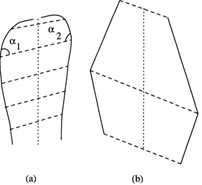
(a)

(b)

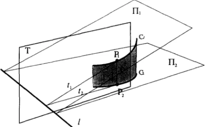
Fig. 5. Examples of (a) skew symmetry with curved contours, (b) and skew symmetry with straight contours. The dotted curves are axis of symmetry and the dashed lines are lines of symmetry. Theorem 2.1. Curves C1 and C2 obtained by cutting a ZGC surface S by two non-parallel planes /71 and /72 project as line-convergent symmetric curves such that the lines joining the corresponding points of the image curves are the projections of the rulings of S and the line I formed on the image plane by joining the intersection points of the tangent lines of the line-convergent symmetric curves is the projection of the 3-D intersection line of the planes HI and/72.

Proof. The above theorem is visualized in Fig. 6. The key to the proof of this theorem is that the tangent plane, plane T, in Fig. 6 of the ZGC surface S is the same along the rulings of S. Therefore, both the tangent lines, tl and t2, of the curves C1 and C2 from points P1 and P2 are on plane T. Also the tangent line tl is on plane /71 and t2 is o n / 7 2. Therefore intersection of tl a n d t2 is necessarily at the intersection point of the three planes/71, /72 and T. For other rulings the same things repeat for a different T plane, and all the tangent line intersections take place along the line l, the intersection line for planes H1 and/72. Hence, on the image plane too the intersection of the tangents takes place on the projection of the line 1. []

Note that the reverse of this theorem, that line-convergent symmetry curves

must come from non-parallel planar cuts of ZGC surfaces, is not valid. How- ever, we believe that it is reasonable to infer that line-convergent symmetry

(8)

F. Ulupmar, R. Nevatia /Artificial Intelligence 67 (1994) 1-28

Fig. 6. Formation of the line-convergent symmetry with a ZGC surface and two non-parallel planes.

curves are planar cross-sections o f Z G C surfaces, if they are terminated by line segments (corresponding to the rulings). For a ZGC surface to produce line-convergent symmetry with non-planar cuts, the cuts must be in a very specific direction, considerably decreasing the probability o f a non-planar cut.

3. Constraints on surface shape

We will solve the recovery of shape from contour problem as a constraint minimization problem. The constraints discussed here are the building blocks of constraints and error terms o f the minimization. The constraints are originally stated in gradient space. However, the gradient space is not uniform, i.e., a constant shift at the center of the gradient space corresponds to a larger vector difference in 3-D than the same shift somewhere further away from the center. For the constraints discussed, the uniformity o f the constraint function implies that the error returned by the constraint function, when not satisfied exactly, depends on the 3-D vector differences rather than the differences in gradient space. When minimization on the gradient space points is employed, the minimization terms should actually be on 3-D angle differences not on Euclidean distances on the gradient space. The purpose o f the normalization is to eliminate the nonuniform contributions by the gradient space points. A gradient (p, q) corresponds to a 3=D vector o f v = (p, q, 1 ). The projection of v on the unit sphere is given by

1

vs = ( p , q , 1). (1)

~/p2 + q2 + 1

The vector vs is the normalized (i.e., Ivsl = 1 ) form of the vector v, and Vs is only dependent on the orientation o f the vector v, it has no length information. Eq. (1) shows that a constant shift in parameters p and q o f vs has less significance, i.e., affects the components o f Vs less, as p and q get

(9)

F. Ulupmar, R. Nevatia/Artificial Intelligence 67 (1994) 1-28 9

F

N 1

F

x1

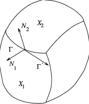
Fig. 7. T w o curved surfaces meeting along a curve F.

larger. The normalized constraint error functions are formulated to compensate for this behavior o f gradient space. The drawback of this normalization is that linear constraint functions are no longer linear.

There are three basic constraint equations that are used in the shape recovery process. We call them the shared boundary constraint, the orthogonality constraint, and the equality constraint. Shared boundary and equality constraints are derived from geometry, the orthogonality constraint is derived from perceptual observations. We first state the constraint and give the equation o f the constraint, then we give a reformulation of the constraint such that the error given by the constraint is uniform and normalized, i.e., in the range [0, 1.0]. 3.1. Shared boundary constraint (SBC)

This constraint relates the orientations of the two surfaces on opposite sides of an edge. The planar version o f this constraint has been used since early days in polyhedral scene analysis [9]. Shafcr et al. [12] first extended it to the case o f intersection of curved surfaces.

Consider two surfaces Xl (u, v ) and X2 (u, v ) meeting along a curve F (s) = ( x ( s ) , y ( s ) , z ( s ) ) as in Fig. 7. Let N l ( u , v ) and NE(U,V) be the normals o f

X 1 and X2 respectively. Along the curve F (s) we can represent the normals

N1 and N2 as Ni(s) = N i ( u i ( s ) , v i ( s ) ) . Let the normals N~(s) be represented in p - q space as Ni(s) = (p~(s),qi(s), 1). In [14] we prove the following constraint:

(10)

10 F. Ulupmar, R. Nevatia /Artificial Intelligence 67 (1994) 1-28

( x ' ( s ) , y ' ( s ) , z ' ( s ) ) . ( ( p z ( s ) , q z ( s ) , 1) - ( p l ( s ) , q l ( s ) , 1)) = O,

x ' ( s ) ( p 2 ( s ) - p l ( s ) ) 4- y ' ( s ) ( q 2 ( s ) - ql(s)) = O. (2)

We call this the shared boundary constraint (SBC) which states that along the curve F (s) the orientation of the surfaces X1 and X2 are constrained by the tangent, (x' (s), y' (s)) of the image of the curve F (s) under orthographic projection. Specifically, the line joining N1 (s) and N2 (s) must be orthogonal to the tangent of the image of the curve F (s).

A stronger constraint can be obtained if we can assume that the intersection curve, F , is planar. Say, F lies in a plane with orientation (Pc, qc)- With the assumption of planarity the constraint equation becomes

x'(s)(Pc - p ( s ) ) + y'(s)(qc - q ( s ) ) = O. (3)

For ZGC surfaces, we will assume that the parallel or line-convergent symmetric curves are planar.

The normalized form of this constraint is a nonlinear equation and it is applied between two gradients (Pl, ql ) and (P2, q2), and a 2-D vector ( x , y ) . The constraint is

S B C ( p l , ql, P2, q2, x, y ) -- ((P2 - P l ) X -I- ((/2 - ql)Y) 2

( ( p 2 - - P l ) 2 -I- ( q 2 - q l ) 2 + 1)( X2 + y 2 ) " (4)

3.2. Orthogonality constraint

The orthogonality assumption has been used in various forms by many authors, based on the belief that the human visual system prefers certain orthogonal interpretations. It was first studied for skew symmetric planar contours by Kanade [7]. We will assume orthogonality between the axis of parallel symmetry and the lines of parallel symmetry. For a ZGC surface, this is equivalent to slicing the surface along rulings to obtain thin skew symmetric planar strips and assuming that these strips are orthogonally symmetric in 3-D. We justify the orthogonality by observation of human perception. A circular cylinder cut by a non-orthogonal plane is, for example, perceived as an orthogonal cylinder [14 ]. In [ 14 ] a detailed discussion of the orthogonality assumption is provided which is omitted here.

Consider Fig. 8, on the surface analyzed, say the image of the tangent vector A makes an angle a with the horizontal and the image of the tangent vector B makes an angle fl at some point on the surface, such that A and B are hypothesized to be orthogonal in 3-D. Let the normal of the surface be N = (p, q, 1 ) at that point. Since the 3-D tangent vectors A and B lie on the tangent plane of the surface they can be represented as

A = (cos(a),sin(t~),pcos(c~) + qsin(t~)),

(11)

I . A - " ,

| I ;

..\ /

Fig. 8. Orthogonality constraint.

From the orthogonality of the 3-D vectors A and B we get A . B = 0; this is the equation o f a hyperbola in the p - q plane since

c o s ( a - f l ) + ( p c o s a + q s i n a ) ( p c o s f l + q s i n f l ) = 0. (6) As in the case o f the shared boundary constraint, this constraint is not normalized either. The normalized constraint is a function of two image directions (Xl,yl) = ( c o s ( a ) , s i n ( a ) ) , (x2,Y2) = ( c o s ( f l ) , s i n ( f l ) ) a n d the surface gradient (p, q) given by

O ( p , q , x l , y l , x 2 , y 2 ) = ( ( x l , Y b P X l + q Y l ) " (X2,Y2,PX2 + qY2)) 2

[(Pl, ql, 1)12l (p2, q2,1)l 2 (7) 3.3. Equality constraint

This constraint is applied when two gradients are hypothesized to be equal. For two gradients (Pl, ql ) and (P2, q2) the unnormalized constraint is

[(Pl,ql) - (PE, q2)l = 0. (8)

Since the gradient space is not uniform, using Euclidean distance between vectors (Pl, ql ) and (P2, q2) is not a normalized and uniform error measure. Therefore, the square o f the sin o f the 3-D unit vectors corresponding to the gradients (Pl, ql ) and (P2, q2) is used:

(12)

12 F. Uluptnar, R. Nevatia /Artificial Intelligence 67 (1994) 1-28

Eq(Pl,ql,P2, q2) = 1 - ((Pl,ql, 1). (P2, q2, 1)) 2

[ (Pl, q], 1 )lZl(p2, q2, 1

)12.

(9)

4. Analysis of ZGCs cut by non-parallel planes

In order to be able to include the contributions of the constraints from each surface and the inter-surface constraints into a pool of constraints, an appropriate parameter representation for each surface is necessary. The parameterization we use is described below.

4.1. Parameterization o f surfaces

For planar surfaces the gradient space representation (p, q) of the surface normal of the plane is used. This is the natural and most versatile (for our purposes) representation for planar surfaces.

In the following we discuss the parameterization and computation of local surface normals, for the case of ZGC surfaces cut by non-parallel planes. As discussed in Section 2.2 a ZGC surface cut by parallel planes produces parallel symmetric curves and a ZGC surface cut by non-parallel planes produces line- convergent symmetric curves. The non-parallel cut case is the more general case.

In order to compute line-convergent symmetry between two curves on a general ZGC surface we must try all possible monotonic point correspondences between the curves. This is a very costly search. However, for the case of cylindrical and conic surfaces, the computation of line-convergent symmetry is much simpler. Most of the ZGC surfaces that we encounter in our environment are in fact cylindrical or conic surfaces. It is known [4] that a ZGC surface consists of cylindrical, conic and tangent surfaces. Tangent surfaces are quite uncommon in the real world, therefore we concentrate on cylindrical and conic surfaces. To ease the job of symmetry finding, a general ZGC surface can be segmented into cylindrical and conic surfaces. However, the constraints and solutions are modeled for a general ZGC surface. Also, there is no problem with over-segmentation as long as the constraints are properly identified between surfaces. The suggested segmentation is along the rulings that passes through the inflexion points of the cross-section curves. The main reason is that, a ruling which passes through the inflexion point of a cross-section curve has the property that the intersection point of this ruling with any curve on the surface is an inflexion point of the curve. This property indicates that inflexion points of two cross-section curves correspond (in the sense of symmetry), providing a corresponding point pair without computing symmetry. Moreover, empirically, inflexion points of the cross-section curves are good candidates for the change of surface type.

A rigorous segmentation can be obtained if a robust linear correspondence line-convergent symmetry finder can be developed. Such a symmetry finder can

(13)

F. Uluptnar, R. Nevatia /Artificial Intelligence 67 (1994) 1-28 1

13

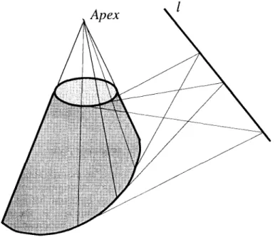
Fig. 9. A conic surface with line-convergent symmetry.

decide on a segmentation point when the symmetry correspondence becomes nonlinear.

For conic surfaces correspondence of line-convergent symmetry is restricted to be along the lines that pass through a common point, the apex of the cone. In Fig. 9 line-convergent symmetry is shown for a cone. The computation of line-convergent symmetry for conic surfaces is, therefore, restricted to checking the correspondences between the curves such that the rulings, when extended, intersect at a single point on the image plane. The process is further simplified when the end points of the curves are available. In that case the apex point can easily be computed on the image plane and it is only needed to check the correspondence for that apex point. For cylindrical surfaces the apex point is at infinity, therefore, the direction of the apex is used rather than the location of it.

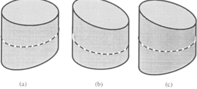
To recover the local surface normals for ZGCs cut by non-parallel planes, we need to decide which cross-section curve is to be made orthogonal to the rulings. Fig. 10 shows three possibilities. In (a) the general preference is to make the top cross-section curve orthogonal, in (b) the bottom one is preferred and in (c) we prefer the middle curve, which is the axis of line-convergent symmetry. In our implementation the curve that "looks" orthogonal to the image axis, which is the line joining the mid-points of the lines joining the end points of the line-convergent symmetry curves, is chosen as the curve that will be made orthogonal. How orthogonal a curve looks is determined by the angle between the image axis and the line joining two ends of the symmetry curve.

(14)

14 F. Uluptnar, R. Nevatia /Artificial Intelligence 6 7 (1994) 1-28

(a) (b) (c)

Fig. 10. Three ZGCs cut by non-parallel planes.

allel symmetry), has three degrees of freedom if no assumptions are used. That is, after the constraints are applied without any assumptions of orthogonality or regularity there remain three parameters to be fixed before local surface normals can be computed at all points on the surface. In the more general case of ZGC surfaces cut by non-parallel planes two additional parameters are involved: the gradient of the second cross-section plane. In total a ZGC surface cut by non-parallel planes has five degrees of freedom. Of the five degrees of freedom, four parameters are the gradients

(Pt, qt)

and ( ~ , qb) of the top and the bottom planes cutting the ZGC surface. The fifth parameter is discussed below. Here we use a slightly different parameterization and approach for computing surface normals than the one we proposed in [14]. This formulation permits the computation of local surface normals of ZGC surfaces at random locations without computing the surface normal at all points on the surface. This property is needed in the combined shape recovery algorithm.

We can model a conic surface by using any 3-D axis that goes through the apex of the cone. We use the 3-D axis that projects as the 2-D axis of the straight edges of the cone. If the image direction of the axis is

(ax,ay),

then the 3-D direction of the axis in gradient space representation is

(Uax, uay),

where u is a free variable; this is the fifth parameter of the ZGC representation. Given (pt, qt), (Pb, qb), and u, the surface gradient can be computed at any point on the surface. In the next subsection we discuss the computation of the local surface normals of a ZGC surface for a particular instance of its parameters.

4.2. Recovering a ZGC surface from its parameters

Consider Fig. 11, let

(Pt, qt)

be the gradient of the cross-section plane that is chosen to be made orthogonal to the surface. The gradient (p, q) of the surface along the ruling r is given by the combination of the two linear constraints given below. The first one is the shared boundary constraint, given in Section 3.1, between gradients (p, q) and (Pt, qt) using the tangent

(x',y')

of the intersection curve at the point the curve touches the ruling r. The

(15)

F. Ulupmar, R. Nevatia /Artificial Intelligence 67 (1994) 1-28 15 ' (XtiP'Ytip) ( P r , q r J / /// (a×,a)) ~ P t , q t ) (Pt,q.t)//// -'~ (Xp,yp)

/j/

/±(x',y')

Fig. 11. The parameters of a ZC_~ surface and the constraints in the gradient (p, q) of the surface

along the ruling r.

equation of the constraint is

( P - - P t , q - qt)" (x',y') = 0. (10)

This constraint is shown in the gradient space by the line labelled ± (x', y') in Fig. 11.

The second constraint is that the 3-D gradient (Pr, qr, 1 ) of the ruling r must be orthogonal to the 3-D gradient, (p, q, 1 ), of the surface along ruling r, that is,

(p,q, 1). (Pr, qr, 1) = 0. (11)

In Fig. 11 this constraint is shown by the line labelled ± (Pr, qr), which is the orthogonal line of the gradient (Pr, qr), i.e., the gradient of the set of the directions that are orthogonal to (Pr, qr) in 3-D. Note that this line is also orthogonal to the 2-D direction of the image of the ruling.

From (10) and (11) the gradient (p,q) of the surface along the ruling r is

given by x'Ptqr + Y'qtqr + Y' p ~-- qrX' -- PrY' (12) 1 + P r P q ~ - -qr

The gradient (Pr, qr) of the ruling r is obtained by reconstructing the axis

line (ax,ay), and the line between points ( x , y ) and (xp, yp) in 3-D (i.e.,

computing the z-coordinates of these image points). Since the gradient of the

axis line is (Uax, uay ), fixing zp = 0, the z-coordinate of the point (xtip, Ytip ),

(16)

Xtip - Xp

zti p -- ( 1 3 )

/,/ax

The z-coordinate of the point ( x , y ) is computed, using the gradient (Pt, qt), a s

z = p t ( x - Xp) q- q t ( Y - Y p ) . ( 1 4 ) Then the gradient (Pr, qr) of the ruling is given by

1

(Pr, q r ) - - - - (Xtip - X, Ytip - Y )- ( 15 )

2ti p -- Z

These formulas are exactly the same for ZGCs cut by parallel planes. In that case the result is independent of the parallel symmetry curve used.

Compared to the case o f a Z G C surface cut by parallel planes, for a ZGC surface cut by non parallel planes there are two additional unknowns, which are the gradient parameters o f the second cutting plane. Also, there are two additional constraints on the orientation o f the planes cutting the ZGC surface. These constraints are not needed to compute the local surface normals of a ZGC surface. In fact the gradient o f the second plane (i.e., the plane that is not chosen to be made orthogonal to the surface) is not needed at all for that purpose. However, since for the multiple-surface recovery algorithm the gradient of the second plane is needed so are these constraints. Here we state the constraints, they will be used in Section 5.1.

The first one is a shared boundary constraint; for a ZGC surface S, with line-convergent symmetry, let (Pt, q t ) be the gradient of the top plane, let (Pb, qb) be the gradient of the bottom plane, and let the intersection line have direction

(lx, ly)

on the image plane. Since the top and the bottom planes actually intersect each other along the line 1 in 3-D we have the shared boundary constraint:

SBC(Pt, qt,Pb, qb, lx, ly)

= 0. (16)

Consider Fig. 12; let (Pr, qr) be the local surface gradient of the surface S along ruling r. This constraint enforces that the 3-D lines tl and t2 be on the same tangent plane having gradient (Pr, q r ) . The constraint is:

tl x r = t2 × r; (17) or in long form: (XI -- X , y l -- Y , - - ( P b ( X l -- X ) + q b ( Y l -- Y ) ) ) X (X 2 - - X I , Y 2 - - Y l , - - ( P r ( X 2 - - X 1 ) -I- q r ( Y 2 - Y l ) ) ) -- ( X 2 - - X , y 2 -- Y , - - ( P t ( X 2 -- X ) + q t ( Y 2 - - Y ) ) ) X ( X 2 - - x l , y 2 - - Y l , - - ( P r ( X 2 - - X l ) + q r ( Y 2 - - Y l ) ) ) , ( 1 8 )

(17)

F. Ulupmar, R. Nevatia /Artificial Intelligence 6 7 (1994) 1-28 17

( x l , y l )

t 2 (x2,y2)

1 : (lx,ly)

Fig. 12. Constraints on the orientation of the cutting planes of a ZGC surface.

Fig. 13. The telephone example.

5. Combined shape recovery

Many objects of interest consist of several curved surfaces. Here the recovered 3-D individual surfaces must be in agreement with the neighboring surfaces, i.e., surfaces sharing a c o m m o n boundary. We describe a technique for such an integrated multiple surface recovery for objects consisting of planar and ZGC surfaces. Figs. 1 and 13 show some sample objects. In the previous section we discussed parameterization of the surfaces and computation of the local surface normals from the parameters of the surface. In this section we discuss a method that sets the parameters of every surface that would be consistent with the neighboring surfaces. The problem of finding a consistent shape for all the surfaces is formulated as a constraint optimization problem, where the shared boundary constraints between surfaces are satisfied exactly and minimization is performed on assumption-driven constraints of orthogonality of surfaces.

The shape o f all the surfaces is recovered simultaneously by finding appropriate values for the parameters of each surface. The values of the surface

(18)

parameters are computed by solving the following constraint minimization problem:

minimize Ei subjectto Ex = 0, (19)

where Ei stands for error terms resulting from internal constraints of each surface and the Ex are the external terms, that is, the constraints obtained by intersection of surfaces.

5.1. Internal constraints

The internal constraints are the constraints obtained from the regularity assumptions of each surface. In general they have the following form:

Ei = Z 2/3pEp -1- Z ~/)°E° + Z z°cEc' (20)

where each w is a weight and Ep is the error term for the orthogonality constraint of the planes, Eo is the error term for the orthogonality constraint of the ZGC surfaces and E¢ is the error term for the implicit constraint of the parameters of ZGC surfaces. These error terms are described in more detail in the following.

Ep is the error term for the orthogonality constraint of planes. If a planar surface has a skew symmetry, then this is the orthogonality function of the lines and axis of skew symmetry as given in (7), where

( x l , y l )

and (x2,yz) are the image directions of the lines of symmetry and the axis of symmetry and (p, q) is the gradient of the plane, wp is the weight of Ep and is proportional to the total length of the contour enclosing the surface. The formula used for Wp is wp =

x/lc

where lc is the total length of the curve enclosing the surface. If the surface does not have skew symmetry Ep is zero.

Eo is the error term for the orthogonality of ZGC surfaces. As in our previous work on ZGC surfaces [14 ], we choose to make the directions of the rulings orthogonal to the tangents of the parallel or chosen line-convergent symmetry curve in 3-D:

1

Eo = -~ y]~ 0 (Pi,

qi, X[,

y~,

Xtip -- Xi, Ytip -- Yi

).

(21 )

i

Here O(.) is the orthogonality constraint given in (7) for i 6 [0, N - 1 ], at the i th location;

(Pi, qi)

is the local surface normal represented in gradient space, (x~, y~) is the tangent of the line-convergent symmetry curve that is chosen to be orthogonal to rulings,

(xi, Yi)

is the location of the point where the ruling meets with the line-convergent symmetry curve, and ( X t i p , Y t i p ) is the location

of the apex of the cone. These are denoted as (p, q), (x', y' ), (x, y), (xtip, Ytip ) respectively in Fig. 11. However computing Eo requires the computation of the local normal at each point on the surface at each iteration of the minimization, which is very time-consuming. Also, since it is a huge nonlinear expression, it creates many local minima around the true minima, where the minimization

(19)

routine gets stuck. Therefore from our experiments we use an approximation of Eo, Eo, such that/~o is quadratic and the error given by/~o is very similar to the one given by Eo./~o has the following form:

/~o = Eax + Et. (22)

Here E~, = cos 2 (a), where a is the angle between the gradient (Pt, qt) of the plane containing the parallel (or line-convergent) symmetry curve that is decided to be made orthogonal and the direction of the image axis (ax, ay ) of Fig. 11. Motivation for E = is based on the observation that the m i n i m u m of Eo in general occurs when (Pt, qt) of Fig. 11 is along a line in p - q space that passes through the origin and is parallel to the image axis. Et = (Uint- u) 2, where u is the u-parameter of the ZGC surface and Uint is set at the initialization by minimizing the orthogonality error Eo given in (21 ). In our implementation we tried both Eo and/~o. It turns out that/~o performs better (in the sense of stability) because it is a simpler error function and creates fever local minima. One can use /~'o as an initializer for Eo, but in our experiments another run of minimization with Eo over/~o was not necessary, wo is the weight of the orthogonality term and is proportional to the total length of the perimeter of the surface, Wo = v/~, where lc is the total length of the contour enclosing the surface.

Ec is the error term for implicit constraints of the parameters of ZGC surfaces. Let

(Pt, qt)

and (Pb, qb) be the gradients of the planes containing the two parallel (or line-convergent) symmetry curves of the ZGC surface. If the ZGC surface has a parallel symmetry, then (Pt, qt) should be equal to (Pb, qb ), therefore, E¢ = Eq (Pt, qt, Pb, qb ), where Eq ( ) is given in (9). If the ZGC surface has an line-convergent symmetry, then Ec is the addition of the constraints given in (16) and (18). Wc is the weight and is inversely proportional to the eccentricity of the parallel (or line-convergent) symmetry curves. If the parallel (or line-convergent) symmetry curves are highly eccentric, i.e., they are almost straight, then the weight of this constraint is low. The formula for Wc = 1/ecc, were ecc is the eccentricity of the total cross-section curve. (The eccentricity of a curve is given by x/~/e2 where el and e2 are the first and second eigenvalues of the covariance matrix of the curve given in (29).) 5.2. External constraints

External constraints are the inter-surface restrictions imposed by each surface on neighboring surfaces. Extremal constraints have the following form:

Ex =

E

wppEpp + E wpzEpz +

E w=Ezz, (23)

where w O is the weight of each constraint and is equal to V~c where lc is the length of the curve produced by intersection of the surfaces. Epp, Epz and Ezz are the error terms for shared boundary constraints between planes,

(20)

between planes and ZGC surfaces, and between ZGC surfaces respectively. In the following, the individual error terms are given in detail.

Epp is the error of the shared boundary constraint between the gradients of the two intersecting planes as given in (4).

Epz is the error term for the shared boundary constraint between a plane and a ZGC surface. There are two possibilities: the intersection is along a ruling of the ZGC surface or the intersection is along a parallel (or line-convergent) symmetry of the ZGC surface. If the intersection is along the ruling of the ZGC surface, then Epz is the shared boundary constraint as given in (4) between the gradient of the plane and the local surface normal of the ZGC surface at the ruling of intersection. If the intersection is along one of the parallel (or line-convergent) symmetry curves, then

Epz = Eq(p,q,Pt, qt) (24)

where (Pt, qt) is the parameter of the ZGC surface, that is, the gradient of the plane containing the intersection curve, and (p, q) is the gradient of the planar surface.

Ezz is the error term for the shared boundary constraint between two ZGC surfaces. There are various ways two ZGC surfaces may intersect each other. Here we only handle the intersections that produce a planar intersection curve. There are two types of such intersections: along the rulings of the ZGC surfaces or along the parallel (or line-convergent) symmetry of the ZGC surfaces. If the intersection is along the rulings of the ZGC surfaces, then the shared boundary constraint given in (4) is applied between the local surface normals of the ZGC surfaces at the ruling of the intersection. If the intersection is along the parallel (or line-convergent) symmetry curves, then let (Px,ql) and (P2,q2) be the gradients of the planes containing the intersection curve in the representations of the first and the second intersecting ZGC surfaces. The error term is:

Ezz = Eq(pl, ql,P2, q2). (25)

When two ZGC surfaces intersect each other along their parallel symmetry (or line-convergent symmetry) curves, how orthogonal both surfaces can be made depends on how parallel their image axes are. Therefore we form a new orthogonality error term Eon for the intersecting ZGC surfaces to replace their original orthogonality error terms (the Eo). Let a be the angle between the image axes of these surfaces, let Eol and Eo2 be the error terms for the orthogonality of the intersecting ZGC surfaces. Then the new combined orthogonality error term is

Eon = cos 2 (a) (Eol + Eo2) + sin 2 (~) (EolEo2). (26)

Eon emphasizes the orthogonality of both of the ZGC surfaces when the image axes are almost parallel to each other, and it emphasizes the orthogonality of either of the ZGC surfaces when the image axes are almost orthogonal to each other.

(21)

5.3. Solving constraint equations

The total error function E is solved using a constraint minimization technique, where Ex consists of "must-satisfy" external constraints and Ei consists o f assumption-driven error terms as defined earlier. To solve this constraint minimization (where the constraints are nonlinear), the problem is converted into a minimization form as follows:

lim min E = lim min (Ei + 2Ex),

2--*inf 2---*inf (27)

that is, E is minimized for successively larger values of 2, thus, emphasizing Ex more at each minimization cycle. At the end, Ex constraints are satisfied almost exactly and Ei constraints are minimized to the extent possible. In our implementation we increased 2 from 1 to 100 in exponential steps of 3.5 (that is 2 = 1, 3.5, 12.25, etc.). For the minimization, a gradient descent algorithm is used. The set of parameters o f the surfaces ( (p, q)'s and u's) minimizing E is taken as the solution set and used to reconstruct the local surface gradients.

Initial values o f the parameters of E, i.e., the parameters of all the surfaces involved in E, are computed by an initializer. The initializer starts with an arbitrary Z G C surface, and sets its parameters as if it is an isolated surface. Then the initializer sets the parameters of the neighboring surfaces by keeping them consistent with the first surface, and the neighbors of these surfaces are processed progressively until the parameters o f all the surfaces are initialized.

6. Implementation and results

For the results shown in this section the following implementation is used. The input to the program are segmented curves--represented as a list of points--that define the contour o f each object. However we do not assume that the input curves are noise-free. These segmented curves are grouped into closed regions using continuity. Each closed region is taken to correspond to an object surface. Next, we find symmetries among segments o f a surface. Every segment bounding a surface is checked for symmetry (parallel, line- convergent or skew) against every other segment in the surface. Two segments are considered to be symmetric, if they return a

low

symmetry error defined for each of these symmetries. For parallel symmetry the symmetry error is given by

12

1 f ~(x~(s)_x~(ps))2 + (yi(s)_y~(ps))2ds,

(28) 0

where the segments Cl(S) =

(Xl(S),yl(s))

and C2(s) =

(x2(s),y2(s))

are parameterized in terms o f their arc length s, p =

ll/12

is a sealing parameter where ll a n d / 2 are the lengths o f the segments C1 and C 2.

(22)

E l

C2 "'",,,,,.

ix, y i) ... The fitted line "",.,,,

Fig. 14. Computation of line-convergent symmetry.

Line-convergent symmetry is computed in a similar way. First the apex point of the conic surface is computed using the end points of the two curves that are checked for line-convergent symmetry. Then the correspondences of the points on the curves are given by extending the lines from the apex that intersect both of the curves. Let { ( x i , Y i ) } be the set of the intersections of the tangents of the corresponding points on the two curves CI and C2, as shown in Fig. 14. The goodness of line-convergent symmetry is given by how well a line fits to the points { (xi, Y i ) } . The goodness of line fit is computed by computing the scattering matrix of the points as

S = 1 E ( X i _

1E(Xi_X)(yi_y )

y)2 , ( 2 9 )

where (~,y) is the mean of the points { ( x i , y i ) } . The scattering of these contour points is given by the eigenvalues el and e2 of the covariance matrix S (el being the larger one), and the goodness of fit is given by v/~-/e2 . Ponce [11] provides a Hough transform-based approach for computing this symmetry, which is much more expensive in terms of complexity.

The above symmetry computations are effective only if the entire lengths of two segments are symmetric to each other. Also, this measure is limited to parallel or line-convergent symmetry found in cylindrical and conic surfaces only.

(23)

Segments are also checked for having the same curvature sign at the corresponding points. This measure is especially useful when the segments are almost straight, in which case the error measure given in the above equations may be low even if the segments are not parallel or line-convergent symmetric. We compute skew symmetry by performing a one-dimensional search in the direction of the lines of symmetry. For two curves C1 (s) and C2 (s) the algorithm is as follows.

Step

1. Use the direction of the line joining C1 (0) and C2(0) as the initial

direction r.

Step

2. Compute the correspondences of curves C1 and C2 such that the

lines of symmetry

{li}

are parallel to direction r.

Step

3. Compute the mid-points, {

(xi, Yi)

}, of the lines {li}.

Step

4. Fit a line to the points

{(xi,yi)}

by using the method described in

the computation of the line-convergent symmetry.

Step

5. Stop if the error of the line fit is at a m i n i m u m with respect to

direction r. Otherwise move direction r in the m i n i m u m error direction and go to Step 2.

If the final line fit error is low, then curves C1 and C2 are accepted as skew symmetric with r being the direction o f the lines of symmetry and the line fitted in Step 4 as the axis of symmetry.

The surfaces containing a parallel or line-convergent symmetric segment pair are treated as curved and others are treated as planar. For curved surfaces the curves joining parallel symmetric curves are checked if they are straight to confirm that the surface is a ZGC.

Some surfaces are a combination of various curved surfaces and there is no distinctive boundary between them. This is the case for the curved surfaces of the object in Fig. 13. Such surfaces contain more than one parallel (or line- convergent) symmetry and they are segmented into smaller surfaces containing only one parallel (or line-convergent) symmetry. Fig. 15 shows the segmented surfaces and the symmetries (skew, parallel or line-convergent) for each surface. The constraints for each surface and the inter-surface constraints including the ones for the newly formed intersections are extracted forming the error function E. Then E is minimized by the constraint minimization technique discussed in Section 5.3. Figs. 16 and 17 show the output of the steps of the minimization process for increasing A for the objects in Figs. 1 (a) and 13 respectively. For both figures, A-values are 0, 1, 3.5, 12,42 from left to right, top to bottom. A = 0 corresponds to the initial state. The computed surface normals are shown by needle diagrams, as needles sticking to the surface in the direction of the local surface normals. For planar surfaces, a small coordinate frame, with a triangle at the base, is used to better show the computed surface normal. Note that, for the object in Fig. 17 the result of the very first step of the minimization (4 = 1 ) is very similar to the final result. Whereas for the object in Fig. 16 most o f the parameter determination happens at later stages o f the minimization (i.e., for larger k-values). This is because, for the object

(24)

24 F. Ulupznar, R. Nevatia /Artificial Intelligence 67 (1994) 1-28

\

Fig. 15. The segmented surfaces, and the symmetries computed for each surface. The skew

symmetry of planar surfaces is shown by crosses, the long line is the axis of symmetry and the short one is the direction of the lines of symmetry. Parallel and line-convergent symmetries are shown by their curved axes only.

in Fig. 16, the middle surface is initially classified as a curved surface due to the parallel symmetry it has. However, it's perceived as a planar surface affected by the planarity of the top surface as discussed in the Introduction. Therefore, strong inter-surface constraints are needed to force the planarity

A = O A = I A = 3 . 5

A = 1 2 A = 4 2

Fig. 16. Surface normals at the end of each step of the minimization, as 2 increases, for the object

(25)

A = O

F. Ulupmar, R. Nevatia /Artificial Intelligence 67 (1994) 1-28

A = I A = 3.5

25

A = I 2 A = 4 2

Fig. 17. Surface normais at the end of each step of the minimization, as A increases, for the object in Fig. 13.

of the middle surface, and increasing ;t emphasizes inter-surface constraints. T h e final result of the minimization, in fact, shows the middle surface as planar within error bounds of the minimization. For the object in Fig. 17 no surface imposes a drastic shape change, from the initial classification, on other surfaces. Therefore, for this figure, cvcn weaker inter-surface constraints provide a reasonably consistent shape.

Figs. 18 and 19 show the final results for the objects in Figs. I (a) and 13 respectively. This process takcs approximately 2 minutes for an object on a

Fig. 18. The needle and the shaded images obtained from the computed surface normals for the object in Fig. 13.

(26)

Fig. 19. The needle and the shaded images obtained from the computed surface normals for the object in Fig. 1 (a).

Symbolics 3645 computer running in LISP. Besides the needle diagrams, we also provide the shaded images of the objects computed by using the surface normals, a Lambertian reflectance model and a point light source. We believe that the computational results are in agreement with human perception, though we have not attempted a quantitative comparison.

7. Conclusion

We have described a technique for recovering 3-D shape of objects consisting of zero-Gaussian curvature (and planar) surfaces. Our method incorporates the constraints imposed by all the surfaces simultaneously. As shown by an example, this can result in fixing the shapes of some surfaces which are ambiguous otherwise.

We have attempted to show the accuracy of our results by comparison with human perception. For shape from contour analysis, the only

ground truth is

really in human perception, for even if the given contour was obtained by a real object, it

could

have been also obtained by any number of other objects as well. Our system has a certain notion of preference that is based partly on geometrical analysis and partly on perceptual observations (i.e., assumptions). The agreement of the final reconstructed surfaces in the examples with the usual human perception confirms the viability of the perceptual observations, like orthogonality, we have made.

The current system assumes that clean and complete boundaries are given. This cannot be expected to be the case for real objects in complex environments. To cope with these difficulties will require incorporation of some perceptual organization techniques. We believe that our methodology will help in this step too, as we are able to provide strong constraints that hypotheses of a perceptual organization system can be tested against. This is the topic of separate, current research in our laboratory.

(27)

A possible research direction is incorporating n o n - Z G C surfaces. W e have worked on recovery of other types of surfaces such as straight homogeneous generalized cylinders [15] and constant cross-section generalized cylinders

[17]. The main issues are to identify the possible ways such surfaces m a y come together, and to form the necessary constraints between them.

Our current method assumes orthographic projection. Perspective projection introduces various additional problems. The biggest difficulty is that additional ambiguities arc introduced. Parallel symmetry, under perspective, turns into a line-convergent symmetry. Line-convergent symmetry remains line-convergent. Hence, we can no longer distinguish a m o n g the two cases without higher level reasoning. Thc constraint equations themselves can bc generalized for perspective projection as shown in [16]. In fact once the symmctrics arc identified, the perspective analysis provides tighter constraints, thus allowing us to relax other assumptions.

References

[1 ] H. Barrow and J. Tenenbaum, Interpreting line drawings as three dimensional surfaces, Artif Intell. 17 (1981) 75-116.

[2] M. Brady and A. Yuille, An extremum principle for shape from contour, IEEE Trans. Pattern Anal. Mach. Intell. 6 (1984) 288-301.

[3] M.B. Clowes, On seeing things, Artif Intell. 2 (1) (1971) 79-116.

[4] M.P. Do Carmo, Differential Geometry of Curves and Surfaces (Prentice Hall, Englewood Cliffs, NJ, 1976).

[5] R. Horaud and M. Brady, On the geometric interpretation of image contours, Artif. Intell. 37 (1988) 333-353.

[6] D.A. Huffman, Impossible objects as nonsense sentences, in: B. Mcltzer and D. Michie, eds., Machine Intelligence 6 (Edinburgh University Press, Edinburgh, Scotland, 1971 ) 295-323. [7] T. Kanade, Recovery of the three-dimensional shape of an object from a single view, Artif

Intell. 17 (1981) 409-460.

[8] T. Kanade and J.R. Kender, Mapping image properties into shape constraints: skew symmetry, affine transformable patterns, and the shape from texture paradigm, in: J. Beck, B. Hope and A. Rosenfeld, eds., Human and Machine Vision 237-257 (Academic Press, NY, 1983).

[9] A.K. Mack'worth, Interpreting pictures of polyhedral scenes, Artif Intell. 4 (1973) 121-137. [10] V. Nalwa, Line drawing interpretation: bilateral symmetry, in: Proceedings Image

Understanding Workshop, Los Angeles, CA (1987) 956-967.

[ 11 ] J. Ponce, D. Chelberg and W.B. Mann, Invariant properties of straight homogeneous generalized cylinders and their contours, IEEE Trans. Pattern Anal. Mach. Intell. 11 (9)

(1989) 951-966.

[12] S.A. Shafer, T. Kanade and J. Kender, Gradient space under orthography and perspective, Comput. Vision, Graph. Image Process. 24 (1983) 182-199.

[ 13] K.A. Stevens, The visual interpretations of surface contours, Artif. Intell. 17 (1981) 47-73. [14] F. Ulupmar and R. Nevatia, Infering shape from contour for curved surfaces, in: Proceedings lOth International Conference on Pattern Recognition, Atlantic City, NJ (1990) 147-154. [ 15 ] F. Ulupmar and R. Nevatia, Shape from contour: SHGCs, in: Proceedings Third ICCV,

Japan (1990).

[ 16 ] F. Ulupmar and R. Nevatia, Constraint for interpretation of line drawings under perspective projection, Comput. Vision, Graph. Image Process. 52 (1991) 674-676.

(28)

[17] F. Ulupmar and R. Nevatia, Recovering shape from contour for constant cross section generalized cylinders, in: Proceedings Computer Vision and Pattern Recognition Conference, Maui, HI (1991).

[18] I. Weiss, 3-D shape representation by contours, Comput. Vision, Graph. Image Process. 41 (1988) 80-100.

[ 19] G. Xu and S. Tsuji, Inferring surfaces from boundaries, in: Proceedings First ICCV, London (1987) 716-720.