Selçuk J. Appl. Math. Selçuk Journal of Special Issue. pp. 95-108, 20100 Applied Mathematics
Comparison of Some Estimation Methods in Linear Regression A¸sır Genç1,Ümran M. Tek¸sen2, ˙Ilkay Altında˘g3
Selçuk University, Science Faculty, Department of Statistics, 42003, Kampus, Konya, Türkiye
e-mail: 1agenc@ selcuk.edu.tr,2uteksen@ gm ail.com,3ialtindag@ selcuk.edu.tr
Presented in 2National Workshop of Konya Ere˘gli Kemal Akman College, 13-14 May 2010.
Abstract. In this study, we are informed about some methods as alternatives to the classical least squares methods which are used for simple linear and multiple linear regression analysis. In short, linear regression model is shown via matrix as;
= +
where is the vector belonging to dependent variable, is the design matrix of independent variables, is the parameter vector, is the vector belonging to error terms, so the least squares estimator of the linear regression is shown by
ˆ
= (0−10 )
Alternative methods have emerged on the purpose of outliers’ existing in obser-vations unlike the least squares estimation, data’s not providing the regression assumptions or using of the previous information about parameters as well. In the study, we are informed about the least absolute deviations regression apart from the least squares method, artificial neural networks, M-regression, the non-parametric regression and Bayesian regression. On the purpose of comparison of the methods’ results, numerical results are derived by using the tempera-ture variation data in Antalya and Fethiye regions for simple regression analysis and variables affecting the fuel percentage in crude oil for multiple regression analysis.
Key words: Least squares method, least absolute deviations regression, ar-tificial neural networks, M-regression method, nonparametric regression and Bayesian regression.
1. Introduction
The main aim of the regression analysis can be finding correlations by defin-ing the relation between dependent variable and independent variable(s) with mathematical models, and estimating the dependent variable with the aid of the independent variable(s). This study gives information about some methods which can be alternatives to the least squares method which is most used in application for parameter-estimating in simple and multiple linear regression models. Alternative methods are suggested for the cases such as outliers’ ex-isting in observations, data’s not providing the regression assumptions or using the previous information about parameters as well.
The second section of the study mentions the linear regression model and the least squares method. In Section 3, the least absolute deviations method which transacts by using the sum of absolute deviations of the error terms is given. In Section 4, we are informed about the artificial neural networks and the estima-tion of the direct dependent variable. In Secestima-tion 5, M-regression from robust statistics is demonstrated, and in Section 6, the method for nonparametric re-gression application is given. In Section 7, Bayesian rere-gression which enables the using of previous distribution information of parameters is demonstrated. In Section 8 of the study, we are informed about numerical application data and obtained findings. And in Section 9, there are interpretations of the results belonging to the numerical applications.
2. Linear Regression and Least Squares Method
When there is a correlation between dependent variable () and independent variable (), it is expressed with observations as,
(2.1) = 0+ 1+ = 1 2
where it’s assumed that it is ∼ (0 2). 0 1 2 are the parameters to be estimated. The multiple linear regression model can be written as
(2.2) = 0+ 11+ 22+ + + = 1 2
where 1 2 are the explanatory variables which are more than one and is the explained variable. It’s again assumed that the error terms are ∼ (0 2).
vector is orthogonal to each column vector of the = £
1 1 ¤ matrix. Apart from the assumptions on error term, about regression model, there are the assumptions of it’s () = ( = + 1), 0 matrix is a nonsingular matrix and the model has been correctly established. The regression model is expressed with matrix demonstration as
Consider the problem of estimating the ∈ < parameter. When the least squares (LS) method is handled, from the optimization problem;
(2.4) min
( − )
0( − ) = min (
0 − 200 + 00) the equation below is obtained
(2.5) ˆ = (0)−10
The estimator of 2 is,
(2.6) =
0 − ˆ0
−
The error terms related to the model are computed by = − ˆ. One of the criteria used for the exploration of the model’s suitability is the mean square error (MSE) value. This value is computed by
(2.7) = 1 − X =1
And another criterion is the determination coefficient. The determination co-efficient is a criterion for the part of the sum of the change in the dependent variable which is expressed by the regression model, and it’s computed by
(2.8) 2= = P ( ˆ− ¯ )2 P (− ¯ )2 2=
value takes a value between 0 and 1. Its being close to 1 shows that the independent variable defines the dependent variable. Its being close to 0 expresses that the independent variable does not define the dependent variable. The estimator of parameters shall use demonstration instead of ˆ. The hypothesis for the parameters’ significance is established as
0: =
1: 6=
In order to test the hypothesis on significance level, the test statistic is
(2.9) =
ˆ −
√
and has distribution with − degree of freedom. Here, are the diagonal components of (0)−1 matrix. And in || = 1−
2; −, 0 hypothesis
3. The Least Absolute Deviations Method
In the least absolute deviation method (LAD), 0 and 1, the sum of the ab-solute deviations of the residuals is computed by the minimization of theP|| expression. Namely, it is obtained from the solution of
(3.1) minX|− (0+ 1)|
system of equation. There is no formula for LAD estimations. Instead of this, an algorithm is used.
In LAD method, the aim is to find the line which has the least absolute deviation value and which is the most appropriate to the data. The most important part of algorithm, for any given (0 0) point, is the process of choosing the best line among others which pass through this point. LAD regression line should pass through two of the observation points. By taking one of the observation points, for instance (1 1), the best line passing through this point is found. This line also passes through a reordered (2 2) point. Then, the best line passing through (2 2) is found. And this line passes through (3 3), which is a reordered point. Then, the best line passing through (3 3) is found and it continues in this way. While the algorithm continues, the obtained line becomes better. Consequently, the latest line becomes the same as the former one. This line, without considering through which points it passes, is the best line and it’s the LAD regression line. The hypothesis for the test of regression parameter is established as such in LS method.
In simple linear regression, the LAD regression line was passing through two points. Also, in multiple regression which has pieces explanatory variables, LAD regression equation provides the (+1) observation points. And in multiple linear regression application, since theP|| expression is tried to be the least,
(3.2) minX|− (0+ 11+ 22+ · · · + )|
optimization problem is required to be solved. Because there is no formula for minimization, an algorithm is used. In simple LAD regression, the iteration is begun with a line and is continued by finding a better line. The treatment continues until the best line is found. Likewise, the multiple LAD regression is also an iterative method.
In LAD regression, testing the significance of the parameters is performed with the sum of the absolute values of the residuals of the reduced model and entire model. The number of parameters in the entire model is , and it is in the reduced model. By estimating the two models and finding the absolute sum of the residuals, the significance of the ( − ) pieces parameters which create the difference between the two models is tested together [1].
4. Artificial Neural Networks
Artificial neural networks (ANN) is a programming approach which aims to carry the study of the neural network existing in the livings to the electronic environment. Artificial neural networks, as in the livings, are also aimed to have such abilities as learning, remembering, and updating what is learned.
A sample of the simplest neural network is a single-layer and single-nerve per-ceptron. These artificial neural networks have more than one inputs and only one output. The output value is 1 or 0. Perceptrons have been usually used in order to split the objects into two different category.
The conducted researches assert that multiple-layer networks can solve the prob-lems that single-layer networks cannot. The perceptron model with many layers is made up of one input, one or more intervals, and one output layer. All treat-ment components in one layer are connected with all treattreat-ment components in the next layer.
In the multiple-layer perceptron networks, the network is shown a sample and as a result of the sample, what kind of a result it’ll produce is notified as well (counseling learning). The samples are applied in the input layer, are processed in interval layers (secret unit) and outputs are obtained from the output layer. According to the learning algorithm used, by spreading the error between the network’s output and the desired output backwards, the weights of the network are changed until the error is reduced to minimum [3].
4.1. The Back-Propogation Network Algorithm
Step 1. The weight between the input units and secret units, ’s, and the weight between the secret and output units, ’s, are started by choosing little random numbers.
Step 2. By choosing a sample, the treatment of forward spread is done. For this, first, the secret unit values are computed by using the equation below,
(4.1) = ( ) = 1 1 + −
where, it’s defined as,
(4.2) =
X =1
shows the weight from input unit to secret unit, shows the value of the input for sample, shows the number of input knots. Then, the output unit values are computed by using the equation below,
(4.3) ˆ= ( ) = 1 1 + −
where, it’s defined as, (4.4) = X =1
shows the number of secret units, , shows the weight from the secret unit to the output unit.
Step 3. After the output values are computed, the treatment of backward spread is done. Primarily, the output errors are computed by the equation below,
(4.5) = (− ˆ) ‘(ˆ)
Then, the secret layer errors are computed by the equation below,
(4.6) =
X =1
(1 − )
Step 4. For being used in updating the weights,
(4.7) ∆v() =
(4.8) ∆w() =
equations are obtained. Here, is learning ratio (0 1) free from assay. By benefitting from the equations (4.7) and (4.8), the new values of and are obtained as
( + 1) = ()+∆v()
( + 1) = ()+∆w()
Step 5. The steps above are iterated for each of the samples. According to the error criterion denoted by = 12
P =1 P =1
(− ˆ)2, the iterations are repeated until convergence occurs.
5. M-Regression
M-regression and LAD regression are both from robust statistics. A statistic process’ being robust means that even when the assumptions of the statistical model are not provided, it can produce a good result. For example, if the data is appropriate to the normal linear regression model, the least squares method gives a good result. But when the error terms are not appropriate to the normal distribution assumption, it’s not a robust statistic. M-regression is a special robust statistic used for the case of this assumption’s being not appropriate. M-estimator tries to choose the 0and 1parameters so as to make theP(ˆ) expression the least. It’s a function of (), . The least squares and the least absolute deviations methods, () = 2 and () = || respectively, are the special cases of M-estimator.
Huber’s M-estimator uses a () function which finds an interval way for 2and ||. The function is defined as
(5.1) () =
2
− ≤ ≤ 2 || − 2 −
If Huber’s M-estimators are viewed as 0 and 1, they try to make the
(5.2) X(− (0+ 1)) equation the least.
As in simple regression, in multiple linear regression as well, Huber’s M-estimations are the 0 1 values which make the
(5.3) X(− (0+ 11+ · · · + ))
equation the least. The function is defined again as in simple regression. The regression parameters vector viewed as is obtained primarily by the least squares method. These values, also in simple M-regression, are used while com-puting the errors which are used in assessing ’s improved estimations and ’s estimation. The algorithm continues in this way until ’s improved estimations become the same with or very close to the previous step. The hypothesis estab-lished as in LS method for the test of parameters is produced by the error terms which are obtained according to the model in which all parameters appear and the function in reduced model [2].
6. Nonparametric Regression
One of the conditions required by the parametric statistic process is the pro-vision of the assumption of appropriateness of random errors to a particular
distribution. And a nonparametric process gives good results for nearly all pos-sible distributions of the errors. Most nonparametric processes are based on the idea of observations’ using their sequences instead of them.
In order to compute the slope of an appropriate line representing the observation points, the slopes of all data pairs should be computed and a value like mean or median should be found from those. The slope of the line combining ( ) and ( ) points is = (− )(− ). (because the slope shall be undefined in case of = , it’s neglected) ’s the least squares estimator can also be denoted as ’s weighted mean.
(6.1) ˆ =X
Here, it’s = (−)2P(− )2. The hypothesis for the test of parame-ters is like it is in LS method. The test statistic can also be obtained depending on sequence numbers of the error terms.
The nonparametric estimations of the 1 parameters for multiple regres-sion are the values which make the
(6.2) X ∙(− (11+ · · · + )) − + 1
2 ¸
×(−(11+· · ·+)) equation the least. By using the estimations obtained from this equation, 0 is obtained by
(6.3) − (11+ · · · + )
The ˆ= − (11+ · · · + ) errors in (6.3) are assessed by
(6.4) X ∙(ˆ) − + 1 2 ¸ ˆ
The minimization treatment is alike. 0 estimation is based on − (11+ · · · + ) differences and is equal to 0+ . It gathers around 0.
7. Bayesian Regression
The theorem which Thomas Bayes suggests for computing the conditional prob-abilities constitutes the base of the Bayesian approach. According to this the-orem, when the probability of A event’s occurrence is known, computing the probability of B event’s occurrence is also possible. The Bayesian approach which was used in accordance with the aim told above for a long time, was begun to be used in deciding techniques in the ensuing years. The basic prin-ciple of the Bayesian approach can be summarized as all available reasonable information should be analyzed.
The Bayesian approach has been used for such aims as performing more effective parameter estimations in regression techniques as well and especially making the error squares mean the least. But in most studies performed, the biggest lack is the numerical applications’ being insufficient.
Consider = + ¯. ¯shows the mean values of observations. A prior distrib-ution which is given the value, and’s expected values and, and their standard errors and is established. Let and’s prior distributions be independent. The Bayes estimations of and becomes as viewed in (7.1) and (7.1). (7.1) = ˆˆ − ˆ ¯ (7.2) =ˆ " −2 −2 +P(− ¯)2 # + " P (− ¯) −2 +P(− ¯)2 # ˆ (7.3) =ˆ " −2 −2 + # + ∙ −2 + ¸ ¯ ˆ
is ’s the least squares estimator. It’s in the form of ¯ = ˆ. The hypothesis for the test of regression parameter is established as it is in LS method. In order to perform hypothesis test in the Bayesian approach, instead of computing the test statistic and its value, the probability is computed according to the posterior distribution under the accuracy of the 0hypothesis. Consider the multiple linear regression model (2.2). the Bayes estimator of the parameter vector becomes ’s expected value in the posterior distribution. Namely, it’s in the form of
(1) ˆ = ∗ −1 + ∗0 ˆ Here, it’s (7.5) ∗= (−1+ 0)−1
is the variance-covariance matrix obtained from the prior information, and are the ˆ
estimation values computed from the prior information. In order to test the parameters, the value of the parameters’ posterior distribution is computed [1].
8. Application
As an application data for simple linear regression model, monthly tempera-ture values measured Antalya and Fethiye between 2000-2006 years are taken. A regression model is wanted to be established between the temperature val-ues of these two regions. The treatment is performed by taking the valval-ues of Fethiye region as dependent variable ( ), and the values of Antalya region as independent variable ().
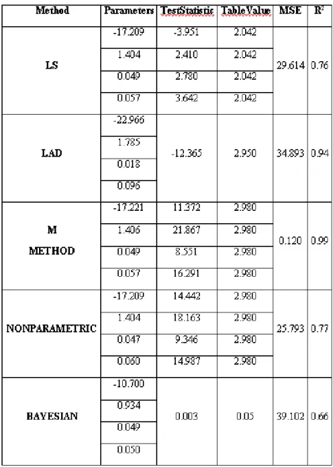
In Table 1, parameters belonging to the least squares and the alternative meth-ods, the validation of parameters, and the error squares mean values of the model are given. The graphic of the estimations obtained from each method against observations is seen in Figure 1.
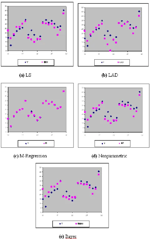
Table 1. Model summary table about methods in simple linear regression For multiple linear regression model as well, by using the variables affecting the fuel percentage in crude oil, numerical results are reached. The dependent variable ( ) is the fuel percentage in crude oil; and the independent variables are the vapor pressure of the crude oil (1), the temperature at which %10 of the crude oil evaporates (2), and the temperature at which the whole crude oil evaporates (3). The observation number is 31.
Figure 1. Comparison of the estimation values belonging to methods with observations
Figure 2. Comparison of the estimation values belonging to methods with observations
9. Result
According to simple linear regression results, the method which has the max-imum determination coefficient (97%) is M-regression method. According to MSE criterion, the least value (0.869) has been obtained by LAD method. Ac-cording to this, it can be said that the robust methods represent the data bet-ter. From the graphics in which the observation values were given by the each method in the Figure 1, this case has been seen.
According to the multiple linear regression results, the method which has the maximum 2 value (99%) is the M-regression method. The minimum MSE value (0.120) has also been obtained by the M-regression method for the multiple linear regression data. When also the graphics in the Figure 2 are examined, it has been seen that the estimations gained by the M-regression method are highly appropriate with the observation values.
In all the methods used, the parameters have been seen to be significant. It can be decided by considering whether the handled data provides the regression assumptions or not that which method is more appropriate.
References
1. Birkes, D., Dodge, Y. (1993), “Alternative Methods of Regression”, John Wiley & Sons,Inc., Canada.
2. Çetin, M.C., Orsoy, A., (2001), “Do˘grusal Regresyonda Sa˘glam Tahmin Ediciler ve Bir Uygulama”, Anadolu Üniversitesi Bilim ve Teknoloji Dergisi, Vol. 2, No. 2, pp. 265-270.
3. Elmas, Ç., (2007), Yapay Zeka Uygulamalar, Seçkin Yaynclk, Ankara.
4. Genç, A., (1997), “Çok De˘gi¸skenli Lineer Olmayan Modeller: Parametre Tahmini ve Hipotez Testi”, Ankara Üniversitesi Fen Bilimleri Enstitüsü Doktora Tezi, Ankara.