High resolution time-frequency analysis by fractional domain warping

(1)

HIGH RESOLUTION TIME-FREQUENCY ANALYSIS BY FRACTIONAL DOMAIN

WARPING

Ahmet Kemal Ozdemic Liitjiye Durak and Orhan Arikan

Department

of

Electrical and Electronics Engineering,

Bilkent University, Ankara, TR-06533 TURKEY.

Phone: 90-3 12-2664307, Fax: 90-3 12-2664192

e-mail:

{kozdemir,

lutfiye, oarikan}@ee.bilkent.edu.tr

ABSTRACT

A new algorithm is proposed to obtain very high resolution time-frequency analysis of signal components with curved time- frequency supports. The proposed algorithm is based on fractional Fourier domain warping concept introduced in this work. By in- tegrating this warping concept to the recently developed directionally smoothed Wigner distribution algorithm [ I], the high perfor- mance of that algorithm on linear, chirplike components is ex- tended to signal components with curved time-frequency supports. The main advantage of the algorithm is its ability to suppress not only the cross-cross terms, but also the auto-cross terms in the Wigner distribution. For a signal with N samples duration, the computational complexity of the algorithm is O ( N log N ) flops for each computed slice of the new time-frequency distribution.

1. INTRODUCTION

Time-Frequency (T-F) analysis is the primary tool for the analysis of non-stationary signals. Among various T-F representations, the Wigner distribution (WD) is the most prominent one [2]. The WD of a signal z ( t ) is defined as

W z ( t ,

f )

= / z ( t

+

t ’ / 2 ) 2 * ( t - t’/2)e-jZnft’ dt’ . (1) For linear T-F components, the WD gives the highest auto-term concentration. However, since it is a bilinear representation, it suf- fers from severe cross-term interference in the presence of more than one signal components. The geometry of the cross-terms is analyzed in [3]. As discussed in that reference, even for mono- component signals, there will be cross-term interference if the signal has a curved time-frequency support. Thus cross-terms of the WD can be divided into two categories. We will call the cross-terms due to the interaction of different signal components (i.e., autwomponents) in a multi-component signal as cross- cross terms and we will call the cross-terms due to the interaction of a single signal component with itself as auto-cross terms. The a u t m r o s s terms are also called as inner interference terms [3].

The cross-terms usually interfere with the autwomponents. Therefore they decrease the interpretability of the WD. Thus to have a practically useful time-frequency representation, these cross-terms should be suppressed. Much of the research effort in time-frequency analysis is devoted to design of distributions

0-7803-7041 -4l01/$10.00 02001 IEEE

which give a better description of the signal’s joint time and frequency content. Until recently, most of the algorithms suffered from a trade-off between sharp auto-term concentration and reduced cross-term interference, or they were computationally very expensive to be useful in practical applications. In [I], we developed a novel T-F analysis algorithm: directionally smoothed Wigner distribution (DSWD) which avoids the usual trade-off between the aut+term concentration and cross-term interference for linear, c h i p l i k e autmomponents by performing directional smoothing of the WD slices on the T-F support of the components. However, the auto-cross terms of components with non-linear T- F support could only be partially suppressed by the DSWD algorithm [ 11. In this paper, to alleviate this problem, we incorporated a novel fractional Fourier transform domain warping technique to DSWD. The resultant algorithm gives a very good description of the signal’s T-F distribution by suppressing not only the cross- cross terms but also the auto-cross terms. When digitally imple- mented, the complexity of the algorithm is only O ( N log N ) flops for each slice of the T-F distribution to be analyzed for a signal with N samples duration. In the next section we introduce the concept of fractional domain warping.

2. FRACTIONAL DOMAIN WARPING

Time domain warping is a useful tool which has found place in a diverse set of applications such as speaker and speech recognition [4], transversal filtering with non-uniform tap spacing [ 5 ] , synthesis of time-varying filters for frequency varying signals [6] and time-frequency signal decomposition [7]. Mathematically, it is the operation of replacing the time dependence of a signal z ( t ) with a warping function C(t). For the invertiblity of the warping operation, [ ( t ) is chosen as a one-toone and differentiable function.

Time warping is especially useful in the processing of frequency modulated (FM) signals with arbitrary frequency modu- lation. A typical member of this class of signals is in the form of z ( t ) = A(t)e3’=“‘), where A ( t ) is the nonnegative amplitude and

4 ( t )

is the phase. The energy of these signals in the time- frequency plane is localized around their instantaneous frequency defined as

fz

( t ) = d+(t)/ dt, which is a single valued function of time as shown in Fig. 2(b).

Ideally, the warping function for the FM signal should be cho- sen as the inverse of its phase, < ( t ) = +-‘(fst), where fs

>

0 is

(2)

an arbitrary scaling constant. With this choice, the warped fbnction takes the following form

z < ( t )

= A(((t))e"""f"t

,

which is a sinusoidal function at frequency fs with envelope

A ( < ( t ) ) . Consequently, the algorithms designed to operate on sinusoidal signals can be utilized on the warped signal.

In this paper, we first extend the time domain warping concept to fractional domains [8]. That is instead of warping the time signal z ( t ) , we propose to warp its fractional Fourier transform (FrFT), which is defined as [9, IO]:

z,(t) E { P z } ( t )

4

K,(t,

t ' ) z ( t ' )

dt' , (3)

where a E R is the order of the transformation and K, ( t , t' ) is the kernel of the transformation given in [IO]. A number of interesting properties of FrFT can be found in [IO]. In this paper, we make use of its rotation property which states that, the WD of the ath order FrFT of a signal is the same as the WD of the original signal rotated by an angle of a n / 2 radians in the clock-wise direction [lo]. For instance in Fig. 2(a) and Fig. 2(b), supports of the WDs of a signal z ( t ) and its FrFT ~ ( - ~ . ~ ~ ) ( t ) are shown. The importance of these figures in terms of warping is the following: Although time- domain warping is not useful for the processing of z ( t ) , since this signal does not have a singled-valued instantaneous frequency, it is perfectly well suited to its (-0.75)'h order FrFT. Therefore the fractional domain warping extends the class of signals for which warping concept is applicable.

In the next section, we introduce the application of fractional domain warping to the T-F analysis of curved time-frequency components.

.I

3. WARPED TIME-FREQUENCY ANALYSIS Warped time-frequency analysis begins with the identification of

the signal support in the T-F plane. However if there are more than one signal component or if the signal components are curved, then the existence of cross terms might impede the accurate identification of the signal support in the time-frequency plane. Therefore the supports should be identified by using a reduced cross-term interference [I I ] or a cross-term free distribution [12]. For the sake of clarity, in the rest of this section, the case of a mono- component signal with a curved time-frequency distribution is in- vestigated. When there exist more than one signal components, the same analysis is carried out for each of these components.

The steps of the algorithm will be illustrated on a synthetic signal given in Fig. l(a). As shown in Fig. I(b), the WD, W 3 : ( t , f),

is cluttered with the auto-cross terms. Although the auto-term of the WD is still visible in this example, in a more complicated signal, it is very difficult to obtain useful information out of the WD. Therefore, in Fig. 2(a), the support of the T-F distribution of z ( t )

is obtained by using [12]. With this support information, it becomes clear that a fractional domain warping is more appropriate than the time domain warping. The order n. of the FrFT is chosen such that after an/:! radians rotation of the time-frequency distri- bution of z ( t ) in the clock-wise direction, any line parallel to the frequency axis intersects the rotated signal support no more than

once. For this example, the orientation of the signal support shown in Fig. 2(a),Justifies the use of a = -0.75 as the appropriate FrFT order.

After rotation of the signal support by a r / 2 radians, a spine

$ ( t ) is chosen to approximate the frequency center of the signal support as shown in Fig. 2(b). This selection of the spine, in a sense, is an approximation of the instantaneous frequency of the signal z a ( t ) . However spine is a more general concept than the instantaneous frequency, because if the instantaneous frequency takes negative values, then in the proposed algorithm, any of the curves which is parallel to the instantaneous frequency but takes only positive values should be used as the spine. The spine can be found either by using an instantaneous frequency estimation algorithm or by manually marking some of its coordinates (ti, ft),

1

5

i

5

N on the T-F plane and then connecting these points by using an interpolation algorithm. In this paper, for its simplicity the second approach with spline interpolation [ 131 is preferred. Furthermore, the integral of the spine, which will be needed later, can be analytically computed in this way. Note that, the proposed algorithm is robust to variations of the spine from the exact instantaneous frequency. Therefore a very accurate specification of the spine is not necessary.

After identification of the spine, the inverse of the warping function is found by integration:

r(t) = j ) ( t ' ) d t '

,

t l

5

t

5

t N

,

(4)

f-'(t) =

r(t)/f+

+ t l

,

t l

L

t

L

t N

,

( 5 ) where f+ = r ( t N ) / ( t N

-

t l ) is the mean of the spine. Since

$ ( t ) is found by spline interpolation, its integral can be analytically computed [ 131. With these definitions, the warping function

< ( t ) becomes

Since by definition,

$ ( t )

is a strictly positive fbnction,

r(t)

de- fined in (4) is a monotonically increasing function. Hence its in- verse given in ( 6 ) exists and it is unique. In general a closed form expression for < ( t ) may not exist. However, ( ( t ) is a monotoni- cally increasing function similar to

r(t),

therefore any of its value can be easily computed by using a few iterations of a I-D search algorithm, e.g., the bisection method.

Once the warping function ( ( t ) is found, the fractional domain warping is given as z,,c(t) = x a ( < ( t ) ) . In the simulation example, the warped signal computed by using this relation for

a

= -0.75 is shown

in

Fig. 3(a).

In

digital implementation, uniformly spaced samples z,,c(kT), k E

Z,

of z,,c(t) are to be computed from the available uniformly spaced samples x,,

(kT)

of x,(t), where T is the sampling interval. A multitude of inter- polation algorithms exist for this purpose. In this paper the spline interpolator [ 131 is preferred for its simplicity.

After the warping operation, DSWD, W Z a , < ( t , f ) , of the warped signal za,c(t) is computed on the line segment ( A , f+), t l

5

X

5

t N as shown in Fig. 3(b). The use of the DSWD is

appropriate in this application, because after the warping operation, the curved signal component transforms to an almost linear component in the time-frequency plane. Since DSWD efficiently suppresses cross-term interference on linear signal components, a

(3)

high-resolution T-F slice of the warped signal component is obtained.

Following the computation of the DSWD shown in Fig. 3(b), the slice of the time-frequency distribution W,, ( t , f ) which lies on the spine $ ( t ) given in Fig. 2(b) is found as

Wz,

(<(A), $‘(<(A))) = W z a , ~ (A,

f,)

t l

5

A

5

t N . (7)

To compute other slices of the T-F distribution

WZ,

( t ,

f),

we will impose the frequency shifting property on the resultant distribution. In other words, we require that when y,(t) = za(t)e’2“a,t

is only a linearly frequency modulated version of z,(t), the following relation exists between the T-F distributions of these signals:

*z, ( t ,

f

+

A,) =

WYo

( t ,

f)

. (8)

Therefore, to compute the slice of the T-F distribution

W Z a , < ( t ,

f),

which lies on the shifted spine shown in Fig. 2 , instead of warping the signal z a ( t ) , we have to warp its frequency modulated version y a ( t ) . After obtaining the warped sig- nal g c L , ~ ( t ) shown in Fig. 3(c), DSWD of the warped signal which is given in Fig. 3(d) should be computed.

The warped form of the signal y a ( t ) is straightforward to compute, since ya,C(t) = z , , ~ ( t ) e ~ ~ ” ~ ~ ~ ~ ( ~ ) . Thus in the digital implementation, interpolation of the samples zn (<(lcT)) from the uniformly spaced samples z , ( k T ) should be done only once. For any value of A, the above relation between the warped signals

z,,C(t) and y a , c ( t ) should be used. Thus by combining (7) with (8), we obtain

WZ!“

(<(A), A +

+

$‘(<(A))) = WYa,(. (A, f4) I’ 11

5

A

I

tiv .

(9) This relation is used to compute the slice of the distribution Wz, ( t ,

f)

on a curve which is parameterized as ( t ( A ) , f ( A ) ) = (C(A), $(((A))

+

A$). I!ence, for each value of A, the algorithm derived above gives the samples of a different slice of the time-frequency distribution of z,(t). Thus, by using the same algorithm for several values of A+, it is possible to compute the T-F distribution of z a ( t ) on a region of the T-F plane. In the simulated example, the T-F distribution z n ( t ) obtained by using the mapping rule (9) for a set of A+ values is shown in Fig. 4(a).

Finally, to remove the rotation effect induced by the fractional Fourier transformation, each slice of (it, f ) is rotated back by a r / 2 radians in the counter clock wise direction, and the corre- sponding slice of the T-F distribution

ci/,(t,

f ) of z ( t ) is obtained as

t , ( A ) = <(A) cos(a.rrl2)

-

($(((A))

+

A,) sin(n.rr/2) (1 1) f T ( X ) = <(A) sin(o,r/2)

+

($(<(A))

+

A4)cos(o,.rr/2) . (12) In Fig. 4(b), the resultant T-F distribution of z ( t ) , obtained by rotating the T-F distribution W z a ( t , f ) of z a ( t ) given in Fig. 4(a) is shown.

3 5 5 5

4. CONCLUSIONS

An efficient algorithm is developed to obtain very high resolution time-frequency distribution of signals. By utilizing a novel fractional domain warping concept, the new algorithm extends the per- formance of [l] on chirplike signal components to signals with curved time-frequency supports. By suppressing both the cross- cross terms and a u t w r o s s terms, which are inherently present in the Wigner-distribution, it produces a very good time-frequency description for both linear and curved signal components. The high quality of the resultant time-frequency distribution is illustrated with a simulation example.

5. REFERENCES

A. K. Ozdemir and 0. Arikan, “A high resolution time frequency representation with significantly reduced cross- terms,” Proc. IEEE Int. ConJ Acoust. Speech Signal Pro- cess., vol. 11, pp. 693496, June 2000.

T. A. C. M. Claasen and W. F. G. Mecklenbrauker, “The Wigner distribution - A tool for time-time frequency signal analysis, Part I: Continuous-time signals,” Philips J. Res., vol. 35, no. 3, pp. 217-250, 1980.

F. Hlawatsch and G. F. Boudreaux-Bartels, “Linear and quadratic time-frequency signal representations,” IEEE Sig- nal Processing Magazine, vol. 9, pp. 2 1 4 7 , Apr. 1992. M. K. Brown and L. R. Rabiner, “An adaptive, ordered, graph search technique for dynamic time warping for isolated word recognition,” IEEE Trans. Acoust., Speech, and SignaI Pro- cess., vol. ASSP-30, pp. 535-544, 1982.

N.

Meda, “Transversal filters with nonuniform tap spacing,” IEEE Trans. Circuits and Syst., vol. CAS-27, pp. 1-1 1, 1980. D. Wulich, E. I. Plotkin, and M. N. S. Swamy, “Synthesis of discrete time-varying null filters for frequency-varying sin- gals using the time-warping technique,” IEEE Trans. Cir- cuits and Syst., vol. 37, pp. 977-990, Aug. 1990.

M. Coates and W. Fitzgerald, “Time-frequency signal de- composition using energy mixture models,” Proc. IEEE Int. Con$ Acoust. Speech Signal Process., vol. 11, pp. 633436, June 2000.

H. M. Ozaktas and 0. Aytur, “Fractional Fourier domains,” Signal Process., vol. 46, pp. 119-124, 1995.

V. Namias, “The fractional order Fourier transform and its application to quantum mechanics,” J: Inst. Math. Appl., L. B. Almedia, “The fractional Fourier transform and time- frequency representations,” IEEE Trans. Signal Process., vol. 42, pp. 3084-3091, Nov. 1994.

R. G. Baraniuk and D. L. Jones, “An adaptive optimal- kernel time-frequency representation,” IEEE Trans. Signal Process., vol. 43, pp. 2361-2371, Oct. 1995.

L. Durak, A. K. Ozdemir, and 0. Ankan, “An adaptive multi- ple window short-time Fourier transformation,” submitted to IEEE Int. Con$ Acoust. Speech Signal Process., May 2000. vol. 25, pp. 241-265, 1980.

(4)

[ 131 M. Unser, "Splines a perfect fit for signal and image processing," IEEE Signal Processing Magazine, vol. 16, pp. 22-38, Nov. 1999.

[I41 H. M. Ozaktas, 0. Arikan, M. A. Kutay, and G. Bozdagi, "Digital computation of the fractional Fourier transform," IEEE Trans. Signal Process., vol. 44, pp. 2141-2150, Sept. "1 996.

Algorithm 1 The Warped Time-Frequency Analysis Algorithm 1. Identify the support of the components by using [ 121.

2. Compute FrFT samples za ( k T ) from the input samples z ( k T ) by using [ 141.

3. Rotate the obtained support m / 2 radians in the clock-wise direction, and for each rotated support identify a set of points

( t i , + ( t i ) ) on the spine, and obtain the rest of the points on $ ( t )

by using spline interpolation [ 131. 4. Compute

r(t)

=

J:,

$ ( t ' ) dt' .

5 . Define the warping function ( ( t ) = !?'(f,(t - t l ) ) , where

f+ = r ( t N ) / ( t N - t l ) . Compute its samples C ( k T ) by using

a 1-D search algorithm such as the bisection method.

6. Define the samples of the warped signal as z a , c ( ( ( k T ) ) = z , ( k T ) and perform a non-uniformly spaced to uniformly spaced interpolation: z a , ~ ( ( ( k T ) )

+

z , , ~ ( k T ) .

7. Compute y a , C ( k ~ ) = ~ , , C ( ~ T ) ~ J ~ " ~ * C ( ~ ' ) .

8. Compute the samples of the DSWD WYm,< ( m T , f + ) , t l

/ T

5

m

5

t N / T by using [I], where

T

is the sampling interval of

the DSWD slice.

9. The slice of the T-F distribution is

@,(t,(mT), f r ( m T ) )

= wym,< (m@,

f$)

where ( t p ( m T ) , f P ( m T ) ) defines a curve in the T-F plane parameterized with the variable mT:

t , ( m T ) =

C(mT)

c o s ( y ) - ( $ ( < ( m . T ) )

+

A,) sin( -) f T ( m T ) = < ( m T ) s i n ( y )

+

( + ( < ( m T ) )

+

A + ) c o s ( - ) a n d t l / T

5

m

5

t N / T . n7r fl7r 2

2

n7r 0.x 2 5 2 1 5 4 3 2 - 1 1 0 -1 -2 2 - 0 5 0 -A-? n 2 4 6 -5 0 5 time - . ~ time

Fig. 1. (a) Time-domain signal z ( t ) , (b) the Wigner distribution

WZ(t,

f )

of z ( t ) .

Fig. 2. (a) The support of the signal-term in W3:(t, f ) and its orientation, (b) the support of the signal-term in WZ(-o,,5) ( t , f ) ,

the instantaneous frequency of the signal z(-0.75) ( t ) and the spine * ( t ) '

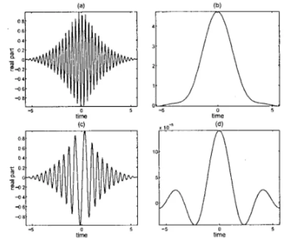
Fig. 3. (a) The warped version Z C ( - ~ 7 R , C ) ( t ) of t h e sig-

nal ~ ( - 0 . 7 5 ) ( t ) ,

(b)

the

DSWD slice

W3:(-o

, s , < ) ( t , f $ )

of

x ( - 0 , 7 s , t ) ( t ) , which gives values of thc T-F l@Z(-o i s ) ( t r f ) lying on the spine shown in Fig. 2(b), (c) the warped version

? & 0 . 7 5 , < ) ( t ) of the signal ?/(-o 7 5 ) ( t ) = ~ ( - o . 7 5 ) ( t ) e J 2 " * * ' ~ , (dl

the DSWD slice WY(-o.,,5,c) ( t ,

f,)

of ~ ( - - 0 . 7 5 , ~ ) ( t ) , which gives

values ofthe T-F

W3:(-o,,s)

( t , f ) lying on the shifted spine shown in Fig. 2(b).

-5

1

-5

time lime

Fig. 4. (a) The T-F distribution

the T-F distribution w,(t, f ) of ~ ( t ) .

i n )

( t ,

f ) o f z ( - o . 7 a ) ( t ) , (b)