GARCH models and an application to stock return volatility with the effect of daily trading volume in Istanbul Securities Exchange

v e

V . . ; ,

-Si ---vr - . ■* " / í* ·: ЯЧ

s 2 ; « * W W ·' ^ é * i *♦ ■ ■ >* '■ Vi«»·«як

GARCH MODELS

AND AN APPLICATION TO STOCK RETURN VOLATILITY WITH THE EFFECT OF DAILY TRADING VOLUME IN

ISTANBUL SECURITIES EXCHANGE

A M aster’s Thesis Presented b y A. TOLGA ÜNAL

to

the D ep artm ent of Econom ics a n d

the Institute of Economics a n d Social Sciences of Bilkent University

in Partial Fulfillment for the D eg re e of

MASTER OF ECO NO M ICS

BILKENT UNIVERSITY ANKARA S eptem ber, 1995

I~l· IS

i U J • U 5 3

T certify that I have read this thesis and in my opinion, it is flilly adequate, in scope and in quality, as a thesis for degree o f Master o f Economics

Assist. Prof Faruk Selçuk

I certify that I have read this thesis and in my opinion, it is fully adequate, in scope and in quality, as a thesis for degree o f Master o f Economics

I certify that I have read this thesis and in my opinion, it is fully adequate, in scope and in quality, as a thesis for degree o f Master o f Economics ^

/

Assist. Prof Erol Çakmak

Approved by the Institute o f Economics and Social Sciences Director:

ABSTRACT

GARCH MODELS

AND AN APPLICATION TO STOCK RETURN VOLATILITY WITH THE EFFECT OF DAILY TRADING VOLUME IN

ISTANBUL SECURITIES EXCHANGE

A. TOLGA ÜNAL Master of Economics

Supervisor: Assist. Prof. Faruk Selçuk September, 1995

In this study, the effect of daily trading volume on stock return volatility is analyzed using the data from Istanbul Securities Exchange (ISE). Generalized Autoregressive Conditional Heteroscedasticity (GARCH) process is employed to model the persistence in volatility of daily returns and to capture the relation between daily price increments and the trading volume. Results approve the consistency of GARCH process in modeling stock returns and indicate positive relation between the volatility of daily returns and trading volume. Also, a reduction of persistence in volatility is observed with the inclusion of trading volume in the model.

Key W ords: ARCH, GARCH, Istanbul Securities Exchange (ISE), Stock Return Volatility, Trading Volume.

o z

GARCH MODELLERİ

VE İSTANBUL MENKUL KIYMETLER BORSASINDA GÜNLÜK İŞLEM HACMİNİN ETKİSİ İLE

HİSSE SENEDİ GETİRİLERİNDEKİ DALGALANMALARA BİR UYGULAMASI

A. TOLGA ÜNAL

Yüksek Lisans Tezi, İktisat Bölümü Tez Danışmanı: Yrd. Doç. Dr. Faruk Selçuk

Eylül, 1995

Bu çalışmada İstanbul Menkul Kıymetler Borsası (İMKB) verileri kullanılarak günlük işlem hacminin hisse senedi getirilerindeki dalgalanmalara etkisi incelenmiştir. Günlük getirilerin dalgalanmalanndaki sürekliliği modellemek ve günlük fiyat artışlarının işlem hacmiyle olan ilişkisini ortaya koymak için Genelleştirilmiş “Autoregressive Conditional Heteroscedasticity” (GARCH) metodu kullanılmıştır. Elde edilen sonuçlar GARCH metodunun hisse senedi getirilerinin modellenmesindeki uygunluğunu onaylamakta ve günlük getirilerin dalgalanmaları ile işlem hacmi arasında olumlu bir ilişki olduğunu belirtmektedir. Buna ek olarak, işlem hacminin modele dahil edilmesiyle dalgalanmalann sürekliliğinde bir azalma gözlenmiştir.

Anahtar Kelimeler: ARCH, GARCH, İstanbul Menkul Kıymetler Borsası (İMKB), Hisse Senedi Getirisi Dalgalanmaları, İşlem Hacmi.

A c k n o w le d g m e n t

I would like to thank Assist. Prof. Dr. Faruk Selçuk for his supervision and guidance during the development of this thesis and would also like to thank Assoc. Prof. Dr. Osman Zaim and Assoc. Prof. Dr. Erol Çakmak for reading and evaluating this thesis.

TABLE ofCONTENTS

1. INTRODUCTION... 1

2. ISTANBUL SECURITIES EXCHANGE (ISE)... 3

2.1. Historyand Structure...3

2.2. An Overviewof ISE-Composite Indexand Trading Volume... 3

3. GARCH MODELS... 5

4. EMPIRICAL APPLICATIONS WITH GARCH MODELS... 10

4.1. GARCH Applicationswith Foreign Exchange... 10

4.2. GARCH ApplicationsWITH Stock Returns... 13

4.2.1. Applications with Stock Returns and Information F lo w ... 16

5. MODEL AND METHODOLOGY... 18

5.1. Estimationand Testingof GARCH Models... 19

6. STATISTICAL FRAM EW ORK... 21

6.1. Stationartty...21

6.2. Unit Roots... 23

7. EMPIRICAL ANALYSIS...25

7.1. The Da t a... 25

7.2. Beta Estimationandthe CAPM... 25

7.3. Unit Roots... 27

7.3. Statistical Findings... 27

7.4. Model Buildingforthe Return Series...29

7.5. Estimationo fGARCH(1,1) Models... 31

8. CONCLUSION...34

T A B L E S... 36

FIG U R E S... 61

1. Introduction

Distributions of speculative price change and rates of return data have important implications for several financial models and are characterized by mild and volatile periods. Two proposed processes. Autoregressive Conditional Heteroscedasticity (ARCH) by Engle (1982) and

Generalized Autoregressive Conditional Heteroscedasticity (GARCH) by Bollerslev (1986) have been shown to provide a good fit for many financial return time series in the literature, allowing volatility shocks to persist over time by imposing autoregressive structure on the conditional variance. This persistence that is consistent with periods of relative volatility and tranquillity in returns is employed to explain the non-normalities in speculative price change and return distributions.

The excess kurtosis of speculative prices such as stock return data as compared to the normal distribution, can in a way be explained by the mixture o f distributions hypothesis: the distribution of rates o f return data appear kurtotic because the data are sampled from a mixture of

distributions that have different conditional variances. This hypothesis supports the price change (or return)-volume tests where the return data are generated by a conditional stochastic process with a changing variance parameter and is substituted by volume. The presence of ARCH effects in daily stock return process can be explained to be based on that the daily returns are from a mixture o f distributions where the daily information arrival is the stochastic mixing variable.' The objective in this study is to examine whether ARCH/GARCH models might capture the time series properties (i.e. serial correlation) of the mixing variable for the daily stock returns and whether ARCH effects disappear when volume is included as an explanatory variable in the conditional variance equation. Using daily trading volume as a proxy for the mixing variable, an empirical strategy is employed to indicate that the volatility of the daily price increments is positively related to the rate of information arrival.

This study is organized as follows. Section 2 gives a brief description of Istanbul Securities Exchange (ISE) and an overview of ISE-Composite Index. Section 3 gives the theoretical framework for the GARCH models and section 4 discusses the literature survey of the empirical applications with GARCH models. Section 5 indicates the model, methodology and the estimation techniques; section 6 describes the statistical properties such as stationarity and unit roots.

2. Istanbul Securities Exchange (ISE)

2.1. History and Structure

With the early 1980’s Turkish capital markets had substantial improvements in both legislative and institutional framework. Following the enaction of Capital Market Law in 1981, Capital Market Board , the institution for setting up the securities exchanges was established. After the publication of “General Regulations for the Establishment of Securities Exchanges and Their Functions” in the Official Gazette in 1984, formally Istanbul Securities Exchange was established at the end of 1985.

ISE operates Monday through Friday and is composed of one main market with a total of 202 stocks traded almost daily. Until June 1990, the ISE had two markets; the Senior Market for 50 actively traded stocks and the Secondary Market for less traded 25 stocks. Expansion of the market necessitated the merger of the two markets in 1990 and the increment of daily trading sessions from one to two in 1994. Currently, ISE operates in a physical market for only equities trading and there are no forward and options markets at present, but with the enhancement of equities trading in Turkey, these type of markets might be considered.

Income from investment in stocks is not taxed and there are no restrictions on foreign investors; the securities market in Turkey is fully open to foreign institutional and individual investors.

2.2. An Overview of iSE-Composite index and Trading Voiume

With the beginning of 1986, officially the first year in operation of ISE, the ISE-Composite Index has increased from 118.87 in February to 170.86 in December and displayed an efficiency of 43.7% with a total trading volume" of 3,273 (thousands) quantities of stocks during the year. The ISE Index at the end of 1987 increased for about 295% compared with year end in 1986, and

Trading volume is considered as the number of shares traded instead of the realized money value herein after throughout the text.

had a level of 675 by December 1987 with the trading volume increment of 350%, reaching a level of 14,731 (thousands) in the same duration. This rapid increase in both the ISE Index return and the trading volume brought ISE to a place that is comparable to stock exchange markets of other developing countries. In 1990, the 50-share ISE Index which reached a all time high of 5,749 till then on August 2, began to slide as the result of a persistent stock price volatility due to the prevailing Gulf Crisis. The year end value of the ISE Index occurred at 3,255 accounting for an increase of 46.8% in 1990. Total trading volume reached to 1,500 (million) shares exceeding the value of 1989 for six times.

In 1991, ISE has structured its main index with two sub-indices; the Financials Index and the Industrials Index. The new cornposite index consisted of 75 company stocks in lieu of the previous 50. Today the calculation of the ISE Index is carried over 100 company stocks. Stock prices displayed significant fluctuations throughout the year despite of the adverse effects of the Gulf W ar in 1991. Generally, price-earning ratios declined but the trading volume increased sharply, ISE Index increased for about 34.2% and the trading volume has risen 2.4 times in 1991 compared with the end of 1990. The impact of the economic crisis in 1994 displayed itself as yielding highly volatile returns and a fluctuating ISE Index; in March, ISE Index dropped to as low as 12,980 level where as it initiated a growing trend in the last quarter of 1994 and closed the year at 27,257 level with an 31.7% increase annually. Daily trading volume displayed an

increasing trend throughout the year, yet nearly doubling its level only two days after the April 5“’ decree.

3. GARCH Models

While it has been recognized for quite some time that the uncertainty of speculative prices, as measured by the variances and covariances, are changing through time, it was not until recently that modeling time variation in second- or high-order moments have been started explicitly in applied researches of financial and monetary economics. One of the most prominent tools that has emerged for characterizing such changing variances is the Autoregressive Conditional

Heteroscedasticity (ARCH) model of Engle (1982) and its various extensions. Following Engle (1982), all discrete time stochastic processes {e,} can be referred of the form

1/2

e, = Zth,

z, i.i.d., E(z,) = 0, v a r(z ,)= l.

(1) (

2

)

with h''~ a time-varying, positive, and measurable function of the time /-1 information set, as an ARCH model. By definition £, is serially uncorrelated with mean zero, but the conditional variance of Er equals /z, which may be changing through time. In most of the applications E, will correspond innovation in the mean for some other stochastic process {y,}, where

y,= g(x,.i;p) + E, (3)

and g(x,.i;P) denotes a function of xm and the parameter vector p, where xm is in time t-l

information set. As proposed by Engle (1982), one possible parametrization for h,is to express hi as a linear function of past squared values of the process.

h, = tto + l^a,E·,.,

1=1 (4)

= tto-H A(L)e‘,

where tto >0, and a,>0 and L denotes the lag operator. This is known as the linear ARCH(q) model. With fin,.ncial data it captures the tendency for large (small) price changes to be followed

by some other large (small) price changes, but of unpredictable sign.

Since the introduction of the ARCH model a vast number of research papers applying this modeling strategy to financial time series data has already appeared. ARCH process of Engle (1982) has been shown to provide a good fit for many financial return time series. ARCH imposes autoregressive structure on conditional variance, allowing volatility shocks to persist over time. This persistence captures the propensity of returns of like magnitude to cluster in time and can explain the well documented non-normality and non-stability of empirical asset return

distributions. While conventional time series models operate under an assumption of constant variance, ARCH allows the conditional variance to change over time as a function of past errors leaving the unconditional variance constant.

In empirical applications of the ARCH model, a relatively long lag in the conditional variance equation is often called for and a fixed lag structure is typically imposed to avoid problems with the negative variance parameter estimates. GARCH (Generalized Autoregressive Conditional Heteroscedasticity), introduced by Bollerslev (1986) allows for both a longer memory and a more flexible lag structure than the ARCH process.

The GARCH(p,q) regression model is obtained by letting the e,‘s be innovations in a linear regression,

E t= yt-x,'b

where y, is the dependent variable, x, is a vector of explanatory variables and is a vector of unknown parameters. Letting e,be a real-valued discrete time stochastic process, and 'F,the information set of all information through time t, the GARCH(p,q) process is given by Bollerslev (1986) as: £ , I % . , - N ( 0 , /zO, (5) ‘I P /2,= tto+ Sa/£^., + 1=1 /=1 (6 )

= qLo + A(L)z‘, + B(L)h,

where p>0, q>0, ao>0, a,>0 (/=1,...,^), p,>0 In order to ensure a well-defined process, all the parameters in the infinite-order AR representation fi, = (1)(L)8·, = (l-p(L))''a(L)e",m ust be non-negative, where it is assumed that the roots of the polynomial P(A,)=1 lie outside the unit circle. For /7=0 the process reduces to ARCH(^) process and e, is white noise for p=q=0.

Asset returns tend to be leptokurtotic; they have a higher kurtosis than that of the normal distribution. In a GARCH model since ai>0, the larger £^is, the larger is h,+], thus large (small) residuals tend to follow large (small) residuals, with the random variation in /i, giving the distribution of £, thicker tails than such random variable Z,, where Z,~ i.i.d., independent of {£,.

Equation (6) also permits rich serial correlation structure for {/z,}, and contributions of trading and non-trading periods to volatility are captured through the tto term.

Engle and Bollerslev (1986) extended GARCH to the class of integrated GARCH (I-GARCH) models that have restriction X a , + XP;=1.1-GARCH(1,1) model sets

/z,= tto+ a i£ ,.i + (l-ai)/iM , (7)

where 0 < a i< l. Based on the nature of persistence in linear models, I-GARCH(1,1) with ao>0 and ao=0 are analogous to “random walks” with and without drift, respectively, and are therefore natural models of “persistent” shocks.

The class of GARCH(p,q) models has been applied to many financial return applications with some success but several authors have felt that these models are too restrictive, because of their imposition of a quadratic mapping between the history of £,and h,. Nelson (1991) claimed that GARCH models impose parameter restrictions that are often violated by estimated coefficients

and that may unduly restrict the dynamics of the conditional variance process." Nelson implied that h, be an asymmetric function of the past data and he modified the conditional variance to

In /i,= tto+ Sp,in

h,.i +

Za, [0\|/,., + y(

-

(2/Tt)''^)] ,

(8)

1=1 1=1

where and a, P, 0, y are constant parameters. By taking the logarithm of the

conditional variance (In h,), it is not necessary to restrict the parameter values to avoid negative variances as in the standard ARCH and GARCH models. This new type of model (8) is called the exponential GARCH (E-GARCH) model. The E-GARCH model is asymmetric because the level of \)/, is included with a coefficient y. Since this coefficient is typically negative, positive return shocks generate less volatility than negative return shocks, all the rest being equal. While this model tries to capture persistent volatility as does the GARCH model, it has two different aspects. First, the log of the conditional variance now follows an autoregressive process. Second, it allows previous returns to affect future volatility differently depending on their previous signs. This is represented by the term in brackets in (8). Assuming is i.i.d. normal, it follows that the innovations £r is covariance stationary provided all the roots of the autoregressive polynomial P(?i)=l lie outside the unit circle.

Many theories in finance involve an explicit tradeoff between the risk and the return. The GARCH-M model is ideally suited to handling such questions in a time series context where the conditional variance may be time-varying. GARCH-M (GARCH-in-mean) processes includes some function of the conditional variance as a regressor in the mean equation, allowing for a consideration of time-varying risk premium. So GARCH-M(1,1) model is set as:

y, = x,'b + yh, + e,

h, = CXo+ OC|£^i-i + Pi^i-i

£, , z ,~ N (0 ,l)

(9) (10)

In this model, the error term, £„ is conditionally normally distributed and serially uncorrelated, and the conditional variance h„ is a linear function of the square of the last period’s errors and of the last period’s conditional variance. This specification of the conditional variance implies

positive serial correlation in the conditional second moment of the serial return process; periods of high (low) volatility are likely to be followed by periods of high (low) volatility. The conditional returns in this model are a linear function of the conditional variance. Under this return-generating process, volatility can change over time and the expected returns are a function of volatility as well as past returns.

In the ARCH(g) process the conditional variance is specified as a linear function of past sample variances only, whereas the GARCH(p,q) process also includes lagged conditional variances. A simple but generally useful GARCH process is GARCH(1,1) given by (5) and

/Z,= tto + OClE^-l + Pl/l,-l, ₍₁₁₎

where ao>0, ai> 0, Pi>0, and a i -i- pi <1 is sufficient for wide-sense stationarity.^ In the

GARCH(1,1) model, the effect of a return shock on current volatility declines geometrically over time. Empirically, the family of GARCH models has been very successful; of these models, GARCH(1,1) is preferred in most cases.®

^ See Bollerslev (1986) for the conditions and proof o f stationarity. ® See survey o f Bollerslev et al. (1992).

4. Empirical Applications with GARCH Models

4 .

1. GARCH Applications with Foreign Exchange

The characterization of exchange rate movements have important implications in international financial applications especially with the second order dynamics. International portfolio

management depends on exchange rate movements through time. Several policy oriented problems about the impact of the exchange rate policies over macroeconomic variables require explanation by exchange rate dynamics.

As is the case with other types of speculative price data, traditional time series models have not been able to capture the stylized facts of short-run exchange rate movements, such as their

periods of stability and volatility. ARCH and GARCH class of models is ideally suited to capture such behavior. Unlike stock returns, the nature of foreign exchange market makes the degree of asymmetry in conditional variances less likely. In the absence of any structural models for the conditional variances, the linear GARCH(p,q) model in (6) therefore is a natural selection for modeling exchange rate dynamics.

As Bollerslev (1987) indicated the distribution of speculative price changes and rates of return data tend to be uncorrelated over time but characterized by volatile and tranquil periods.

Bollerslev used a simple time series model to capture this dependence where the model is an extension of ARCH and GARCH type of models obtained by allowing conditionally t-distributed errors. This development permitted a distinction between conditional heteroscedasticity and a conditional leptokurtotic distribution, either of which as Bollerslev depicted, could account for the observed unconditional kurtosis in the data. Also current conditional variance is allowed to be a function of past conditional variances as in the GARCH model of Bollerslev (1986). In his paper, Bollerslev (1987) used a set of data that consists of daily spot prices from the New York foreign exchange market on the U.S. dollar versus the British pound and the Deutsche mark from March 1, 1980 until January 28, 1985 for a total of 1,245 observations excluding weekends and holidays. He converted spot prices (S,) to continuously compounded rates of return as y,= ln(S,/S,.i) where he indicated that y, series are approximately uncorrelated over time. Bollerslev (1987) concluded

that the results confirm the previous findings in the literature that the speculative price changes and rates of return series are approximately uncorrelated over time but characterized by volatile and tranquil periods.

Hsieh (1989a) estimated autoregressive conditional heteroscedastic (ARCH) and generalized ARCH (GARCH) models for five foreign currencies, using 10 years of daily data, a variety of ARCH and GARCH specifications, a number of non-normal error densities and a comprehensive set of diagnostic checks. The data set consisted of daily closing-bid prices of five currencies in terms of the U.S. dollar-British pound, Canadian dollar, Deutsche mark, Japanese yen and Swiss frank from 1974 to 1983, totaling 2,510 observations. He employed ARCH, GARCH(1,1) and E- GARCH(1,1) models and obtained the results that (i) the standard GARCH(1,1) and E-GARCH (1,1) are extremely successful at removing conditional heteroscedasticity from daily exchange rate movements, and (ii) standardized residuals from all ARCH/GARCH models using the standard normal density are highly leptokurtotic. Hsieh (1989a) also found that E-GARCH fitted the data slightly better than standard GARCH using a variety of diagnostic checks.

Maintaining market efficiency, the ARCH/GARCH effects, present with high frequency data, could be due to the amount of information or the quality of the information reaching the market in clusters, or from the time it takes market participants to fully process the information. Laux and Ng (1993) provided new and more definitive evidence on the mixture of distributions hypothesis where the mixture hypothesis posits that the autocorrelation in the time-varying rate information arrival leads to the volatility dependencies captured by GARCH models. Their paper made use of more theoretically appealing risk specification with appropriate measures of information arrival rate and high frequency data from the futures market than previous investigations of the

hypothesis. Laux and Ng (1993) investigated the explanation of Lamoureux and Lastrapes (1990) that the usual GARCH specification augmented with a volume regressor largely removes GARCH effects, using intraday data on foreign exchange futures contracts traded on the Chicago

Mercantile Exchange (CME).They proposed a simple measure of rate of information arrival, the number of price changes per period that is conceptually close to the number of instances of information arrival per period. An important reason for the setting of information arrival in such a way is that unlike volume, this measure is not sensitive to the precise definition of the scope of the

market. Laux and Ng largely benefit from this assumption since, relevant with their data, foreign exchange futures trading is only a small part of all foreign exchange trade in the market. Their data set consisted of the price of every trade for the five mentioned currencies on the CME during the period December 14, 1982 through December 15, 1986. They measured intraday returns over approximately half-hour intervals as the first difference of the natural log of the final timed price in each half-hour of the trading day. The data set of half-hourly and overnignt returns included

13,169 observations per currency. Laux and Ng concluded with results demonstrating that the univariate GARCH models of foreign exchange futures are misspecified due to the failure to account for the fact that systematic and unsystematic volatilities evolve at different rates with different persistence. Multivariate models demonstrate that autocorrelation in an index of the rate of information arrival, the number of price changes, accounts for a substantial part of the GARCH behavior of unique volatility.

Bollerslev and Domowitz (1993) examined both international patterns of intraday trading activity and the time series properties of returns and bid-ask spreads for the Deutsche mark-U.S. dollar exchange rate in the interbank foreign exchange market. Time series models incorporating various market activity measures were estimated for the mean and variance of the transaction returns, using the data recorded at five-minute intervals.’ Bollerslev and Domowitz treated

“news” effects as dependent strongly on the use of intraday data. Particular news proxies that they employed, include the intensity of the arrival rate of quotations, the size of the bid-ask spread, and the speed of transactions activity measured by the duration between trades. Upon estimating conditional volatility models, they found that the behavior of the bid-ask spread played an important role in determining the conditional volatility of the return process.

The foreign exchange market operates twenty-four hours a day and seven days a week and is one of the closest analogue to continuous time global marketplace. The data set that Bollerslev and Domowitz (1993) used consists of continuously recorded bid and ask quotations for the exchange rate from April 9 to June 30 1989 obtained from Reuter’s network screens for a total of 305,604 quotes. Recent studies generally have used volume or number of transactions as a proxy

for the information arrival process. Given the nature of the data, Bollerslev and Domowitz used the number of incoming quotes as one of their proxies for the information variable. As the

interbank market structure precludes knowledge of the number of transactions and trading volume on the part of traders, the rate of quote arrival is directly observable by the traders. The effect of news on the time series behavior of intraday exchange rate returns, is generally inferred from the behavior of conditional volatility.* Bollerslev and Domowitz (1993) used GARCH(1,1) process to model autonomous movements in the conditional variance employing the assumption on trader’s information by using lagged information on market activity to explain conditional volatility movements. The market activity variables that are employed, included the intensity of quote arrivals, the bid-ask spread and a measure of duration between trades on the temporal

dependencies in the returns process. Bollerslev and Domowitz concluded with the results that, although the trading activity fails to influence the volatility of returns, it affects the uncertainty of trading costs. Also the proposition that the trading intensity has an independent effect on returns volatility is rejected, but it holds for spread volatility.

The results in Engle, Ito and Lin (1990a) with intraday observations on the Japanese yen-U.S. dollar rate showed that except for the Tokyo market, each markets volatility is significantly

affected by changes in volatility in the other markets, therefore the volatility is transmitted through time and different market locations, supporting the information processing hypothesis.

4.2. GARCH Applications with Stock Returns

Volatility in stock return series has many important theoretical implications, therefore there exists numerous empirical applications of the ARCH/GARCH methodology in characterizing stock return variances and covariances.

Akgiray (1989) presented new findings about the temporal behavior of stock market returns and summarized the results of some new time series model applications to daily return series. Akgiray (1989) used the data that contain 6,030 daily returns on the Center for Research in Security Prices (CRSP) value-weighted and equal-weighted indices covering the period from

January 1963 to December 1986, and return is defined as the natural logarithm of the value relatives; i?,= ln(I(//,.|) where dividends are part of the total value. The empirical research on the statistical properties of stock returns that has started with Fama (1965) continued with many other studies have shown that time series of daily stock returns exhibit some autocorrelation for short lags, however these autocorrelations have small magnitudes to form profitable trading rules. After applying regression with OLS method to the return series, Akgiray (1989) fitted two closely related conditional heteroscedastic time series models in order to represent the observed

autocorrelation structure in daily return and squared return series: the ARCH and GARCH

processes. The fact that the conditional variances are allowed to depend on past realized variances in GARCH process is particularly consistent with the actual volatility pattern of the stock market where there are both stable and unstable periods. As Akgiray (1989) indicated, within the class of GARCH processes GARCH(1,1) fitted the daily return series best. Akgiray tried other models such as GARCH (p,q) for p=l,...,5 and q=l,...,3 but no significant improvements in goodness-of- fit based on likelihood ratio tests is obtained. Akgiray (1989) concluded with the result that time series of daily stock returns exhibit significant levels of dependence. Also the conditionally heteroscedastic processes allowed for autocorrelation between the first and second moments of return distributions over time, and fitted to the data satisfactorily.

Pagan and Schwert (1990) compared several statistical models including GARCH and E- GARCH processes for monthly stock return volatility. They concentrated on the stock returns from 1834 to 1925 and compared various measures of stock return volatility. Their results imply that the standard models are not sufficiently extensive and non-parametric methods may be superior for stock returns. Augmenting GARCH and E-GARCH models with terms suggested by non-parametric methods yields significant increases in explanatory power. They concluded that the extension of parametric models in the non-parametric direction (e.g., by adding on Fourier terms) is likely to be a good modeling strategy.

Several empirical studies have documented that stock volatility tends to fall subsequent to an increase in stock prices and rise following a decline in stock prices, an observation attributed to the “leverage effect”. According to the leverage effect, a reduction in the equity value would raise the debt-to-equity ratio, hence raising the riskiness of the firm as manifested by an increase in

future volatility. As a result, the future volatility will be negatively related to the current return on the stock. Cheung and Ng (1992) examined and characterized the cross sectional and temporal relations between stock price dynamics and firm size. In particular they investigated the possibility of an inverse relation between future stock volatility and stock price. They used a set of daily return data that contains 251 AMEX-NYSE stocks for the period of July 1962 and December

1989. Their data of stock returns were adjusted for the stock splits, stock repurchases, or dividends paid during the entire sample period. Cheung and Ng employed E-GARCH(l,2)-in- Mean model with the logarithm of lagged stock price in the conditional variance equation. Using the E-GARCH model they found consistent patterns in time series properties of security returns across firms of different market values. Their results display that the sampled AMEX-NYSE stocks exhibit a negative relation between stock price and future stock volatility, and the leverage effect is stronger for small, as compared to large firms.

The paper of Glosten, Jagannathan and Runkle (1993) extends the research of intertemporal relation between the risk and the return. They used the data set of monthly excess returns on the CRSP value-weighted stock index of the stocks on the NYSE during the period 1951:4 to

1989:12. The results obtained supports a negative relation between the conditional expected monthly return and the conditional variance of monthly return, using a GARCH-M model modified by allowing (i) seasonal patterns in volatility, (//) positive and negative innovations to returns having different impacts on conditional volatility, and (Hi) nominal interest rates to predict conditional variance. Glosten, Jagannathan and Runkle also found that time series properties of monthly excess returns are substantially different from the reported properties of daily excess returns. Results suggest that monthly conditional volatility is not highly persistent and negative residuals are associated with an increase in variance whereas positive residuals are associated with a slight decrease in variance.

Engle and Ng (1993) defined “news impact curve” which measures how new information is incorporated into volatility estimates. GARCH and E-GARCH models, and also a partially non- parametric model are compared and estimated with daily Japanese stock return data. They used daily return series of Japanese TOPIX index for the full sample period from January 1, 1980 to December 31, 1988. All the models used in the paper indicated that negative shocks introduce

more volatility than positive shocks, with this effect particularly apparent for the largest shocks. Results also showed that although E-GARCH captures most of the asymmetry, the variability of conditional variance implied by E-GARCH model is too high.

4.2.1. Applications with Stock Returns and Information Flow

An explanation for the presence of ARCH/GARCH processes is based upon the hypothesis that daily information arrival is a stochastic mixing variable where ARCH might capture time series properties of this mixing variable and daily returns are generated by this mixture of

distributions.’ Lamoureux and Lastrapes (1990) examined the validity of this explanation for daily stock returns. Their empirical strategy exploits the implication of this mixture model that the variance of daily price increments is heteroscedastic-specifically, positively related to the rate of daily information arrival. Lamoureux and Lastrapes restricted their attention to a GARCH(1,1) specification since it adequately fits many economic time series. Their data set consists of daily return and trading volume of 20 actively traded stocks since actively traded stocks are most likely to have a sufficiently large number of information arrivals per day. Lamoureux and Lastrapes concluded that daily trading volume, used as a proxy for information arrival rate, has a significant explanatory power regarding the variance of daily returns and ARCH effects tend to disappear when volume is included in the conditional variance equation. These results imply that the

persistence in shocks to volatility is, in part, a manifestation of the time dependence in the rate of information arrival to the market.

Cochran and Mansur (1993) also confirmed the results of Lamoureux and Lastrapes (1990) where they investigated the effects of cash flow and discount rate proxies on the variability of stock returns including a volume regressor in the conditional variance equation. They used

monthly return data from 1947:1 to 1989:12. Various ARCH and GARCH processes are fitted to the monthly excess returns and the effects to the economic variables on expected excess returns

are determined. By using a GARCH-M(1,1) model they found that for monthly excess returns, GARCH results in part from the time dependence associated with the rate of information arrival to the market.

5. Model and Methodology

As Bollerslev (1987) suggests, ARCH and GARCH models capture the dependence of volatile and tranquil periods of speculative price changes and rates of stock return data although they tend to be uncorrelated over time.'® The presence of ARCH/GARCH effects is based on the hypothesis that daily stock returns are generated by a mixture of distributions, in which the rate of

informational arrival is the stochastic mixing variable. In this study we will mainly follow the framework and methodology of Lamoureux and Lastrapes (1990) and examine whether GARCH models capture the time series properties of daily stock returns with and without the inclusion of this mixing variable. Hence, we will try to obtain a measure of the relation between the rate of daily information arrival to the market and the volatility of daily price increments using the data of stocks actively traded in Istanbul Securities Exchange (ISE).

Using the very often applied GARCH(1,1) process, a model for daily stock returns will be in the form R, = |Im + e„ e,l'PM ~N (0,/z.), hi = Cto+ 0Ci£“,-i + (

12)

(13) (14)

where ao>0, ai> 0 , Pi>0, R, represents rate of return, and |J.m is the mean R, conditional on the past information. If parameters tti, [3i are significantly positive then shocks will persist over time and the degree of persistence is determined by the magnitude of these parameters.

Letting p„ as the intraday equilibrium price increment in day t, 8, is written as:

£i = 2 pi, (15)

i=I

where /, is the mixing variable representing the stochastic rate at which information flows into the

10

market and 8, is drawn from a mixture of distributions, where the variance of each distribution depends upon information arrival time. Assuming that p,·, is i.i.d. with mean zero and variance a" with sufficiently large /„ then from Central Limit Theorem we have 8,1/, ~ N (0,a“/,). Assuming also that the daily number of information arrivals is serially correlated; /, is written as,

lt — k-\· b^L^li-x + M, ₍₁₆₎

where k is constant, £>(L) is lag of polynomial order q and «,is white noise. Defining (O, = E(8^l/,), then CO, = a~l, from above mixture model, and substituting this into (16) yields:

CO,

= <rk + b{L)

co,.i +

(17)

Equation (17) can be represented as a GARCH process to capture the persistence in conditional variance equation. Since it is not easy to estimate /,, we use daily trading amount as a proxy; a measure of the daily information rate that arrives into the market in order to obtain the impact of returns conditional on the knowledge of mixing variable. Therefore equations (13) and (14) is extended as:

8,l('F„,,y,) ~N(0,/i,),

hi= 0.0+

C C i£ ‘',.i + p i / i i - i +

yV,

(18) (19)

Persistence of shocks to volatility will be measured by the sum of tti + pi and the impact of this persistence will be large as tti + Pi is close to unity. The sum of tti + Pi will be small and y>0 if the GARCH effects are sufficiently explained by the information flow that is included as the trading volume in the conditional variance equation, (19).

5 .

1. Estimation and Testing of GARCH Models

In the regression equation like y,= x /b + 8, for a GARCH process, the disturbances 8,’s are white noise, in the sense that they are uncorrelated with mean zero, but they are not independent of each other. Hence OLS is inefficient in this case, a fully efficient estimator which considers the

dependence in variance can be constructed by maximum likelihood. For the maximum likelihood estimation of the GARCH regression model, let z,’= (1, e% , h,.p), X’= (ao, ai,..., a,,,.... Pi,..., P</) and 0e 0 , where 6 = (¿’, X’) is the collection of the unknown parameters to be estimated, with 0 being a compact subspace such that e, possesses finite second order moments. Rewriting the GARCH(p,q) model as:

£, = y t- x /b ,

h, = Zt'X,

the log likelihood function for a sample of T observations (apart from constant) is given as:

LKe) = 7” ' Z/,(0), where /,(0) = -1/2 log h -1/2 K \

For a given numerical value for the parameter vector 0, the sequence of conditional variances can be calculated and used to evaluate the log likelihood function. Then, this can be maximized using the method of Berndt, Hall, Hall and Hausman as described in Bollerslev (1986, p.317) or by other numerical optimization procedures. The numerical optimization of the log likelihood function gives the maximum likelihood estimates of the parameters for the GARCH(p,q) model.

In order to have a formal tests for the presence of ARCH/GARCH, Engle (1982) and Bollerslev (1986) have developed Lagrange Multiplier (LM) tests for these models. A LM test (ARCH test) for oco=,...,=ot<,=0 in an ARCH(q) model can be calculated as TR“ from the

regression of e^ (squared residuals from yi = x /b + 8, regression) on e^-i,..., 8% , where T denotes the sample size. The test LM = TR^ is asymptotically under the null hypothesis that there are no order ARCH effects (the same is also valid for GARCH models).

An alternative but asymptotically equivalent testing procedure is to subject 8", to the standard tests for serial correlation based on the autocorrelation structure, including conventional

6. Statistical Framework

6.1. Stationarity

A stochastic process is said to be stationary in a strict or strong sense if the joint and

conditional probability distributions of the process do not depend on time. A restrictive-butusable assumption is to deal with weak sense of stationary as follows: a process {X,}will be said to be stationary if

E(X,)=|x, Var(X,)=a^x<oo, Cov(X„X,.i)=X, so that a^x=X„

Thus, a stationary process will have a mean and variance that do not change through time, and the covariance between values of the process at two time points will depend only on the distance between these points and not on time itself. If any of the conditions above are not satisfied the process {X,} is considered as nonstationary.

The covariances X, will be called autocovariances and the quantities Ç)s=XjXo will be called the autocorrelations of a process. The sequence pj, i= 0,l,2,..., indicates the extent to which one value of the process is correlated with previous values and the extent to which the value taken at time t depends on that at time t-s.

A time series is said to be stationary with X, = pXf.i + e,, if for any value of t, e, has zero mean and constant variance and is uncorrelated with any other variable in the sequence, more formally:

E(e()=0, E(£^)= <T, E(£,,8v)=0 with t^v

Hence a stationary time series fluctuate around the mean whereas a nonstationary series have a time varying mean and covariance.

A type of nonstationary process is called random walk given as Xt = m + X,.i + £,. It says that the current observation is equal to the previous observation plus a random disturbance term where

E(£,)=|i, E(e‘,)= a ‘, E(e,,£v,)=0 with №v

For a sequence of uncorrelated and identically distributed errors £, with zero means, £, is called a white noise process. For a white noise series the autocorrelation sequence is po=l, p.v=0 with

so the correlogram takes a specific and easily recognized shape. For a stochastic process {X,}, “whiteness” does not imply independence between X,and X,., (unless it is a Gaussian white noise) therefore the process is called strict white noise if, in addition, X, and X,.., are statistically independent. If the process {X,} is strict white noise, the processes {lX/1} and {X^,} are also strict white noise.

Nonstationarity in structural time series models may exhibit itself in the form of trend where the series tend to move in one direction; X, = jX« + £; where £, is white noise disturbance term and the |lt is a stochastic trend,

|X/ = M-m + pM + 'Hfi P( = pM +

in which ri, and are also white noise disturbance terms. The level of the series is given by |X„ while P, is the slope. A time series with a stochastic trend may drift upwards or downwards due to the effects of stochastic or random shocks. Both the variance of the process and the correlation between the neighboring values increase over time implying that long periods of values away from mean value are valid.

In a special case when both T|, and have zero variance the stochastic trend reduces to a deterministic linear trend and so,

X, = )i, + £(, where p, = a + Pr with a = p„

m=0. If m ^ , then the process is called random walk with drift. In both cases e,’s are independent and identically distributed random variables and,

Неге, the mean of the process is a specific function of time. A process of mixed stochastic deterministic trend can also be described as;

X( = oc + (3i + X(.| + £(,

The main assumption here is that the mean of e, series are zero and the stochastic process {e,}is white noise.

A nonstationary series {X,} which can be transformed into a stationary series by differencing d times is said to be integrated o f order d and conventionally denoted as: X, ~ I{d). If, for instance the process is of type

X, = Xm + £„ with £, = р£м + %t,

where is a white noise variable, first differencing of X, gives a stationary series, provided that Ip k l for the model not to be explosive, so X,is 7(1).

6.2. Unit Roots

For the economic time series it is necessary to determine whether or not the series are

stationary in levels or in first, second differences. Considering a first order autoregressive model,

Х, = рХм+£„

where £, represents a series of independent normal zero mean random variables and p is a real number, the AR(1) statement is a random walk process when P=1 and such a process generating X, is nonstationary. The process generating X, is stationary and integrated of order zero if ipi<l. In such a model any shock over £, diminish and will not be permanent. In the presence of a unit root in economic time series, variance of the forecasts increases as a function of time and convergence to a limiting distribution is not observed.

A unit root test proposed by Dickey and Fuller (1979) is based on the order of integration of X, with the null hypothesis that P=1 against the alternative (3<1 and is called the DF test. If the null is true than the first difference of the series (AX, = X, - X,.; = e,) will have a unit root. More formally, the DF test is based on the estimation of

AX, = pX,.| + £„

where the null p=0 is tested against the alternative p<0. The series X, have a unit root when p=0 and the alternative p<0 provides stationarity. Stationarity of the time series above, implies X, ~/(0) whereas failing to reject null hypothesis requires further differencing. The test on the null

hypothesis is based on the asymptotic distributions of the i-statistic since the presence of unit roots disable the usage of usual i-tests and F-tests for testing the hypothesis. Critical values of t- statistic proposed by Dickey and Fuller are tabulated in Fuller (1976), table 8.5.2.

The lack of accounting for the possible autocorrelation in the error process £,, yielded Augmented Dickey-Fuller test (ADF) developed by Dickey and Fuller (1981). The ADF test, including lagged left-hand side variables as explanatory regressors to approximate the

autocorrelation, estimates the equation

p

AX, = a + pt + pX,-i + Ep, AX,.,· + £,, ,= l

The r-statistic ("x) and the testing procedure is same as in the D F test whereas the same critical values apply. The null hypothesis of a unit root cannot be rejected as the "t value is greater than the critical value. Null hypothesis of (|)i (p=

0

),

(|)2

(P=p=0) and

(¡>3

(a=P=p=

0

) should be

compared with the critical values of \ and "x respectively from Fuller (1976) table 8.5.2. If the statistic obtained from the related ADF table is not significant then the series has a unit root and further differencing (at least one more differencing) of the series is required to achieve stationarity.

7. Empirical Analysis

7.1. The Data

The data set consists of the daily return and volume series for ISE-Composite Index (for the period of 1/3/1988 - 28/2/1995 with 1749 observations) and 4 actively traded stocks; EREGLİ (Eregli Demir Çelik), IZDM (Izmir Demir Çelik), КОС (Кос Holding) and YKB (Yapi ve Kredi Bankasi) (for the period of 2/1/1990 - 31/1/95 with 1265 observations). Log of adjusted values of the daily closing prices are used in order to generate daily returns /?,(,) (i=ISE, EREGLI, IZDM, КОС, YKB) as i?,(,)=ln(P,/P(.i), where P,'s are adjusted values inheriting stock splits and

dividends. The daily trading volume series is also transformed to their log levels as denoted by V,. The plots o f daily stock return series are displayed in Figure 1.1-1.5.

7.2. Beta Estimation and the CAPM

The Capital Asset Pricing Model (CAPM) of modern portfolio theory can be expressed as:

(P P ,-r/) = p,(PP„,-r/),

where ERi is the expected rate of return on security i, ER„t is the expected return on the market portfolio (i.e. return on ISE-Composite Index), r/is the risk free rate of return and p, is the beta coefficient, a measure of the extent to which security’s rate of return moves with the market and also a measure of systematic risk that cannot be eliminated through diversification. A volatile security has P

>1

and a more defensive security has (3<1. “

In this section, the extent to which the security rate of returns move with the market and the efficiency of CAPM is tried to be tested. For empirical purposes, the regression over time.

R t (<) = 0t| + Pi R l (m) + (m)

'' CAPM and estimation o f p ‘s are described in detail, in Damodar Gujarati’s “Basic Econometrics”, 2"'^ Edition,

is run for the securities where /?,(oand /?,(„,) are the rates of return on the /"’security and on the market portfolio, and (3,is the market volatility coefficient of the /"'security. Then, /'/estimates of P, are used in the regression over the N securities:

/?i = Ф1 + Ф2Р, + М/,

where /?, is the average rate of return for security / computed over the t observations in the former regression. If CAPM holds statistically, ф

1

= г/, фг= the estimator of ER„ - г/. Also, if CAPM holds, фз in regression equation,

/?,■ = Ф1 + фгР,- + фзСГ, + и„

where a ', is the residual variance of the /"' security from the first regression, should not be significantly different from zero. The estimation of P coefficients yielded the results, displaying slightly high p values for Ri(eregu) (P=1.0563) and Rt(Koc) (P=1.0149) than the market beta and slightly less P values for R,(izdm) (P=0.9780) and Rkykb) (P=0.96405) over 1265 observations. Estimation of CAPM equation gives

Ri= 0.00868 - 0.00662 pi + щ, (0.01753) (0.01746)

R =0.067 DW=2.10

with /-statistics of 0.495 (фО and -0.379 (Ф

2

) respectively. The estimated values for the risk free rate and the market risk premium are insignificant and the value is also low, concluding with the result that CAPM does not hold with at least the estimation carried over for small number of securities. In order to verify the result, estimation with the alternative regression equation is done resulting in

R, = 0.0399 - 0.03308 p, - 3.387a^-b m„ (0.0054) (0.04936) (0.4638)

/-value for фз, significantly different from zero, supports the previous finding that CAPM does not hold for ISE (at least with these cluster securities).

7.3. Unit Roots

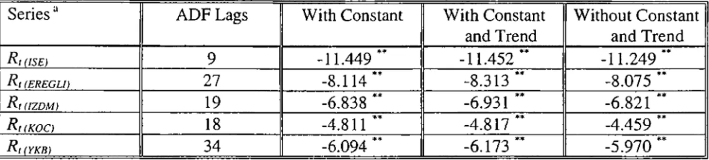
The ADF test for presence of unit roots is applied to the daily return, daily volume and daily growth in volume series. In order to impose that ADF residuals are empirically white noise, optimal lag structures as Akaike and Schwarz criterias are employed to determine the number of ADF lags.‘‘ The tests are repeated for random walk, random walk with a drift and finally with random walk with trend and drift. Table 1.1. displays the results of the test for presence of a unit root for the return series and the results of the five entities indicate stationarity of the return series with R, (,)’s ~ 1(0). The volume series exhibit nonstationarity for the five entities as shown in Table

1

.

2

., where stationarity for the volume series is achieved through first differencing, as is the case in Table 1.3. Therefore we have V, ~ 7(1) for the daily volume series. The critical values for the ADF-i test statistic are taken from Fuller (1976), page 373, Table 8.5.2. and presented in Table 1.4.

7.3. Statistical Findings

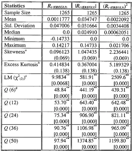
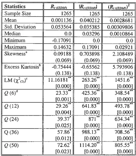
A wide range of descriptive statistics for the return series R,, 17?,I and (7?,)^ (for market return and four securities) and the growth in daily volume series are presented in Tables 2.1. to 2.6. The descriptive parameters are mean, standard deviation, median, minimum, maximum, skewness and excess kurtosis. Statistics in order to test null hypothesis of normality (Lagrange Multiplier test) and strict white noise (Ljung-Box portmanteau test) are also included.

The unconditional sample skewness for RtgsE) exceeds the normal value of zero by 0.75 standard errors. For 17?, (вд! and (7?, (вд)^ the normal value is exceeded by approximately 25 and 56 standard errors. Also the sample kurtosis for RtusE), \Ri(ise)\ and (7?, (¡se))' exceeds the normal value of zero-excess kurtosis by approximately 10, 10 and 19 standard errors. For the securities.

A detailed description of these information criterias can be found in Harvey (1990), Charemza W. W. and Deadman D. F. (1992).

the sample skewness for Rheregu), ^Rkerecld^ and {R, (eregu))' exceeds the normal value by 1.4, 15 and 32 standard errors, whereas the sample kurtosis exceeds the normal value by 3, 2.6 and 37 standard errors; sample skewness for R ,gzdm), \Ri(I2dm)\ and {R, (/zdm))' exceeds the normal value by

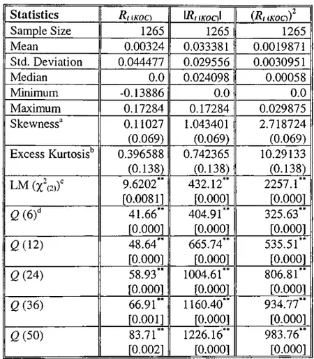
1.3, 10 and 30 standard errors, whereas the sample kurtosis exceeds the normal value by 5.4, 4.8 and 42 standard errors; sample skewness for R,(koo, \Rhkoc)\ and {R, (koo)' exceeds the normal value by

1

.

6

, 15 and 39 standard errors, whereas the sample kurtosis exceeds the normal value by 3, 5 and 74 standard errors; sample skewness for Rhykb), and {R, (YKB)f exceeds the normal value by 4.3, 19 and 119 standard errors, whereas the sample kurtosis exceeds the normal value by 8.7, 26 and

1021

standard errors. As a final result, the return series exhibit both skewness and leptokurtosis.

The Lagrange multiplier test for joint normal kurtosis (zero-excess kurtosis) and skewness (zero skewness) rejects the null hypothesis of normality for R,, I/?,I and (R,)^ for each of the five entities, supporting the common view that daily stock returns are not normally distributed. The Ljung-Box portmanteau statistic is calculated for lags up to 50 days and only those for lags

6

, 12, 24, 36 and 50 are reported in Tables 2.1-2.6. The null hypothesis of strict white noise'^ is rejected for all the return series at the 1% level except Rkizom), where we found 5% significance for lags 24, 36 and 50. The serial correlation in (R if series for the five entities is consistent with a non­ linear return generating process and a non-linear process cannot be strict white noise although it may be white n o i s e .I n Table 2.6. the Ljung-Box statistics for the volume series exhibit high Q- statistics for lags

6

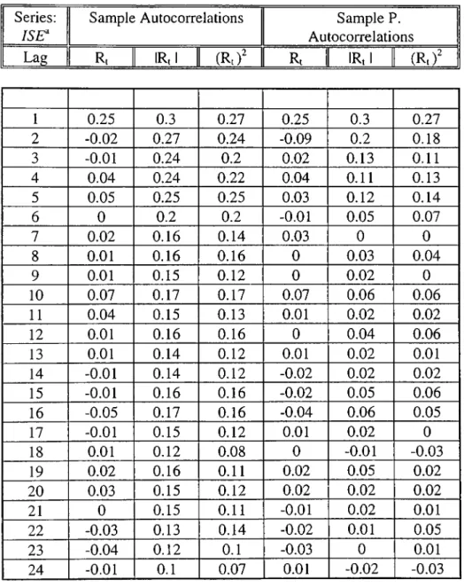
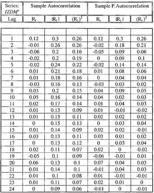
through 50 at 1% level, indicating serial correlation. The result derived is that the daily stock return series are not independent.

In order to deal with this lack of independence in daily returns, the sample autocorrelation functions for the series 7?,, 17?,I and (7?,)^ may be analyzed. The estimated sample autocorrelations and sample partial autocorrelations for the three return series of ISE-Composite Index, EREGLİ, IZDM, КОС and YKB are shown in Tables 3.1-3.5 with the correlation figures 2.1- 2.20. All of the return series exhibit high first-lag autocorrelations ranging from 0.12 to 0.25. Using the

Strict white noise can be defined by independence of R, and also the state of R, being strict white noise implies I/?, I and (R, f being strict white noise.

approximation of as the standard error of these estimates, the first-lag autocorrelations exceed (for R,gsE)), 6 (7 )'''' (for RaEREGU)), (for R ,uzdm)), 5(7)·"' (for R,^eoo) and 5(7)·"' (for R,(YKB))· The autocorrelations in the absolute and squared returns are much higher than those in the return series. Especially the autocorrelations in the absolute return series are generally higher than in the squared returns. Both autocorrelation functions slowly decay as the lag increases (see Figures 2.3, 2.7, 2.11, 2.15 and 2.19, ABS(Return) and SQ(Return) stands for \R,\ and ( R ,f respectively) and significantly positive for lags up to 50 days. The results for

especially absolute returns agrees with the early work of Fama (1965) that large price changes are followed by large changes of either sign. Flence, the autocorrelations for absolute and squared returns indicate the lack of independence and ensure that return series are not strict white noise processes. Another conclusion that can be derived from the autocorrelation structures of the return data is that the squared return data exhibit substantially more autocorrelation than the normal return data, which can be thought as an indication of conditional heteroscedasticity'^ for all return series of the five entities.

7.4. Model Building for the Return Series

As we know from the descriptive statistics of the previous section, return series exhibit both skewness and leptokurtosis. Also, it is shown that the return series are not strict white noise processes and display non-linear ({R ,f) dependence structures. Non-linear dependence may be explained by changing variances which can also explain the high kurtosis in return series.'^

A satisfactory model of daily stock return series must take into consideration the serial correlation in the return series and the non-linear dependence in the return structure (serial correlation in the squared return series). Therefore, a transformation for the return series is required where the new series are uncorrelated. Thus, the model to be fitted for the new return series would satisfy uncorrelated structure for the non-linear series.

This is adapted from Hsieh (1989). See Akgiray (1989).

R, = ^o + + ... + ^pR,.p + £, + Y,e,.| + ... +

hence the residuals of the models can be expected to be uncorrelated. After trying several models according to the sample autocorrelations and sample partial autocorrelations for the return series (from Tables 3.1-3.5), appropriate AR(p) models are obtained as in Table 4.1.

Sample statistics of the AR(p) residuals for the return series are displayed in Table 5.1. Sample skewness for StasE) exceeds the normal value of zero by 0.67 standard errors, whereas the sample kurtosis for e,(/s£) exceeds the normal value of zero-excess kurtosis by 11 standard errors. For the securities, the sample skewness, for Ekeregu), exceeds the normal value by 1.4 standard errors, whereas the sample kurtosis exceeds the normal value by

1.1

standard errors; sample skewness for £/(/zDAi), exceeds the normal value by 0.89 standard errors, whereas the sample kurtosis

exceeds the normal value by 3.67 standard errors; sample skewness for e,(koc), exceeds the normal

value by 1.15 standard errors, whereas the sample kurtosis exceeds the normal value by 2.8 standard errors; and sample skewness for e,(ykb), exceeds the normal value by 3.71 standard errors, whereas the sample kurtosis exceeds the normal value by 9.9 standard errors. These results show that residual series exhibit both skewness and leptokurtosis as the original return series.

The Lagrange multiplier test for joint normal kurtosis (zero-excess kurtosis) and skewness (zero skewness) rejects the null hypothesis of normality for all of the residual series at

1

% level (at 5% level for Et{Koo)·, indicating that residual series are not normally distributed. The Ljung-Box portmanteau statistic is also tabulated in Table 5.1 for lags

6

, 12, 24, 36 and 50 for residuals and the null hypothesis of no serial correlation cannot be rejected at the

1

% level for all the residual series and at 5% for e,(ykb)· The autocorrelation functions of the residual series are displayed in

Figures 3.1, 3.3, 3.5, 3.7 and 3.9 (SQ(Residual) stands for eY) for the five residual series. The squared autocorrelations for the residual series are similar to their counterparts in the return series as shown in these figures. The autocorrelations in the squared residuals are significantly positive

For the reasons stated above, a linear transformation o f return series /?, that generates a new series which exhibit no serial correlation can be modeled as an ARMA(p,^) process:

at even long lags and decay slowly as in the autocorrelations of squared return series. The type of intertemporal dependence in the squared residuals is also clear from the high Ljung-Box-i

2

statistics as in Table 5.2. The null hypothesis of no serial correlation can be rejected for the squared residuals and this supports that the residual series £,are white noise processes.’’

The non-linear intertemporal dependence stated by the high ^ ‘Values and the kurtosis

displayed by the residual series for all the entities together with the results of the ARCH (%’(df=d) tests (from Table 5.1) indicate the appropriateness of a GARCH modeling process for the return series. Also, for a diagnostic check on the application of GARCH processes on the daily return series, the autocorrelation function (ACF) and the partial autocorrelation function (PACF) of the E'l (squared residuals) can be examined (Figures 3.1-3.10). As described in Bollerslev (1986), ACF of an GARCH(p,q) process exhibits oscillatory decay (similar in ARCH(q) process) and the PACF for GARCH (p,q) is in general non-zero but dies out at higher lags (cuts off at lag q in ARCH(q) process). Examining the figures 3.1 through 3.10, the ACF and PACF of the squared residuals display these typical characteristics for the appropriateness of a heteroscedastic process, although the PACF’s display significant positive correlations at initial lags, these die out as the lag increases.

7.5. Estimation of GARCH(1,1) Modeis

After diagnostic checking of the appropriateness of a GARCH process, the following equations are constructed to represent the model for daily return series of the form,

^( = <l

)0

+ + ··· + ^pRl-p + £t. £,l ( 'Pm.F,) ~ N(0,/it),

h,= ao+

a i£ V i + +

yV,

is not Strict white noise since is not a strict white noise process. When the series is non-normal (which is the case for e, here), failure to reject independence hypothesis by LJung-Box test, is the same as failure to reject hypothesis o f white noise; therefore e, is not independent but uncorrelated.

where tto>0, ai> 0, (3|>0, and /?, represents rate of return with AR(p) structure for the daily return series. Using the maximum likelihood estimation method described earlier, the models are

estimated with

7^0

(without volume) first and then with unrestricted у (including volume regressor in the variance equation). Starting with various initial values for the parameters, the global maxima is obtained in the all the models that are estimated. Results excluding the volume regressor are displayed in Table 6.1. Robust standard errors and r-statistics are calculated with estimated coefficients in the sense that conditional normality of errors are not assumed. For all the return series, the sum of GARCH(1,1) parameters (tti + (3i) are all less than unity and the Pi estimates are substantially larger than the a i ’s. These results indicate that the fitted models are second-order stationary and at least the second moments exist.'® The sum of (ai + Pi) are all less than but close to unity ranging from 0.9210 to 0.9788, indicating that the persistence in shocks to volatility is relatively large. The standard error series are skewed and leptokurtotic indicating for non-normal errors. Also, the Lagrange multiplier test for the null of normality of errors is

assumed, failed to accept the conditional normality of errors for all the series at 1% (for ISE, EREGLİ, YKB) and 5% (for IZDM, КОС) respectively. If the G ARCH model completely

accounts for the leptokurtosis in the unconditional standard errors, the distributional assumptions should be satisfied and standard residuals (e,//z'^^) should be normally distributed. Here, in this case GARCH accounts for some, but not all of the leptokurtosis in the daily returns. The Ljung- Box portmanteau statistics for the selected lags (

6

, 24 and 50) exhibit low Q values for both the standard and squared standard residuals indicating the absence of first-or second order serial correlation. Table 6.1 provides strong support that daily stock returns can be characterized by a GARCH(1,1) model when the volume is not included in the variance equation.

In Table 6.2, the results of the GARCH models with volume regressor in the variance equation are displayed. Volume is included as the daily growth rate of volume and exhibits strong serial correlation (as shown in Table 2.6). The estimated results exhibit that the sum of GARCH(1,1) parameters (tti + Pi) are all less than unity (imposing second order stationarity), but the

persistence in shocks to volatility are all reduced substantially when volume is included in the

model. For all the return series, the coefficient of volume(Y) is positive (as expected) and

statistically significant (by the i-statistic displayed). The indicator of persistence to volatility (tti + Pi), has a range between 0.02831 and 0.12686 whereas coefficient of volume (y) has a range between 0.10422 and 0.16580 for the five return series, supporting the hypothesis that GARCH effects are sufficiently explained by the information flow into the market that is included as the daily growth in trading volume in the conditional variance equation. As is the case for the model where volume is not included, the model with volume displays both skewness and leptokurtosis for the standard errors and the Lagrange multiplier test for the null of normality of errors fails to accept the conditional normality of errors for all the series at 1% significance. The Ljung-Box portmanteau statistics for the selected lags (

6

, 24 and 50) again exhibit low Q values for both the standard and squared standard residuals indicating the absence of first-or second order serial correlation indicating the appropriateness of the GARCH model specification with volume.