a thesis
submitted to the department of industrial engineering
and the institute of engineering and science
of bilkent university
in partial fulfillment of the requirements
for the degree of
master of science
By
˙Ibrahim Evren Kahramano˘glu
September, 2006
Assoc. Prof. Dr. Oya Ekin Kara¸san (Supervisor)
I certify that I have read this thesis and that in my opinion it is fully adequate, in scope and in quality, as a thesis for the degree of Master of Science.
Prof. Dr. Mustafa Pınar
I certify that I have read this thesis and that in my opinion it is fully adequate, in scope and in quality, as a thesis for the degree of Master of Science.
Assistant Prof. Dr. Yavuz G¨unalay
Approved for the Institute of Engineering and Science:
Prof. Dr. Mehmet B. Baray
Director of the Institute Engineering and Science
NETWORKS
˙Ibrahim Evren Kahramano˘glu M.S. in Industrial EngineeringSupervisor: Assoc. Prof. Dr. Oya Ekin Kara¸san September, 2006
In this thesis, we consider a robust capacity expansion-routing problem with uncertain demand. Given a network with source and demand nodes and a ca-pacity budget, the caca-pacity expansion problem is related to the determination of the arcs on which additional capacity will be installed in order to minimize the overall routing cost while satisfying the demand of the nodes. We make use of the Robust Counterpart (RC) approach in the literature in order to make capac-ity installation and routing decisions. RC approach is important since it does not allow any constraint violation for any realization of the uncertainty and such approaches are often necessary in engineering applications in real life.
We apply the classical RC formulation to our problem that results in a sim-ple one-stage model. The two-stage version of the RC formulation, namely the Adjustable Robust Counterpart (ARC), is also applicable to our problem. The formulation of the ARC is given but since it is not computationally tractable, an approximation to ARC developed recently, namely Affinely Adjustable Robust Counterpart (AARC) formulation, is applied to our problem and solved.
The efficiencies of the RC formulation and AARC formulation are tested via two different sets of numerical studies in the experimental part. The main model that allows capacity installation in continuous amounts as well as two extensions that make use of the modular capacity approach are used in the experimental study. The computational experiments illustrate that AARC approach provides robust solutions at a much cheaper cost in terms of objective function value when compared to RC approach. In addition the loss of optimality due to application of AARC formulation is minor.
Keywords: Robust Optimization, Capacity Expansion Problem Robust Counter-part, Adjustable Robust CounterCounter-part, Affinely Adjustable Robust Counterpart.
SER˙IMLER ¨
UZER˙INDE DAYANIKLI KAPAS˙ITE
ARTTIRIMI VE ROTALAMA KARARLARI
˙Ibrahim Evren Kahramano˘glu End¨ustri M¨uhendisli˘gi, Y¨uksek Lisans Tez Y¨oneticisi: Do¸c. Dr. Oya Ekin Kara¸san
Eyl¨ul, 2006
Bu tezde talep belirsizli˘gi altında serimlerde dayanıklı kapasite geni¸sletme ve ro-talama problemi ¨uzerinde ¸calı¸sılmı¸stır. Kapasite geni¸sletme problemi, kaynak ve talep noktaları belirtilen bir a˘g ¨uzerinde, verilen bir kapasite b¨ut¸cesinin toplam rotalama maliyetini en aza indirgeyecek ve t¨um talepleri kar¸sılayacak ¸sekilde da˘gıtılması ile ilgilenmektedir. Kapasite b¨ut¸cesinin da˘gıtımı ve rotalama kararları literat¨urdeki “Robust Counterpart” (RC) yakla¸sımı ile verilmi¸stir. Bu yakla¸sım modeldeki hi¸c bir kısıtın ihlal edilmesine izin vermemektedir. S¨oz konusu yakla¸sım ger¸cek hayat uygulamalarında, ¨ozellikle m¨uhendislik alanında, sık kar¸sıla¸sılan bir durumu temsil etmesinden dolayı ¨onem arz ermektedir.
Tek a¸samada dayanıklı bir ¸c¨oz¨um ¨ureten RC yakla¸sımının yanı sıra iki a¸samada ¸c¨oz¨um ¨ureten ve RC yakla¸sımının ¨ozel bir ¸sekli olan “Adjustable Robust Counterpart” (ARC) yakla¸sımı da ¨uzerinde ¸calı¸sılan modele uygulanabilir bu-lunmu¸stur. S¨oz konusu ARC yakla¸sımının form¨ulasyonu verilmi¸s fakat bu uygu-lamanın genellikle kolay ¸c¨oz¨ulemeyen modellerle sonu¸clanmasından dolayı ARC form¨ulasyonunun bir yakla¸sı˘gını sa˘glayan “Affinely Adjustable Robust Counter-part” (AARC) yakla¸sımı form¨ule edilip ¸c¨oz¨ulm¨u¸st¨ur.
RC ve AARC yakla¸sımlarının verimlili˘gi iki farklı sayısal ¸calı¸sma ile test edilmi¸stir. Tam sayı olmayan de˘gerlerde kapasite y¨uklemeye izin veren ana model dı¸sında mod¨uler kapasite yakla¸sımını benimseyen iki ayrı model daha kullanılmı¸stır. Sayısal deneyler sonucunda AARC yakla¸sımının RC yakla¸sımına kıyasla ¸cok daha ucuz maliyetlerle dayanıklı sonu¸clar ¨uretti˘gi g¨or¨ulm¨u¸st¨ur. Ayrıca AARC yakla¸sımı sonucunda elde edilen sonu¸clar belirsizlik olmayan veriler ile elde edilen optimum sonu¸clar ile kar¸sıla¸stırıldı˘gnda kayıpları olduk¸ca azdır.
Anahtar s¨ozc¨ukler : Dayanıklı Serim Tasarlaması, Kapasite Arttırımı. iv
I would like to express my gratitude to my supervisor Assoc. Prof. Dr. Oya Ekin Kara¸san and Prof. Dr. Mustafa Pınar for their instructive comments in the supervision of the thesis.
I would like to express my special thanks and gratitude to Assistant Prof. Dr. Yavuz G¨unalay for showing keen interest to the subject matter and accepting to read and review the thesis.
I would like to express my deepest thanks to my family, my girlfriend, Kay-tarık¸cılar, ¨Onder and his place for their keen friendship, morale support and helps.
Finally I would like to express my special thanks and gratitude to T ¨UB˙ITAK for the scholarship provided throughout the thesis study.
1 Introduction 1 1.1 Uncertain Optimization Problems and Dealing With Uncertainty . 1
1.2 Brief Contents of the Study . . . 3
2 General Definitions and Formulations 6 3 Literature Survey 10 4 Problem Formulation 26 4.1 Notation . . . 27
4.2 Uncertainty Set . . . 28
4.3 Formulation of the Main Model . . . 29
4.4 Formulation of the RC Model . . . 32
4.5 Formulation of the ARC Model . . . 33
4.6 Two Cases in Which ARC, RC and AARC are Equivalent . . . . 35
4.6.1 Case 1 . . . 35
4.6.2 Case 2 . . . 37
4.6.3 The Considered Case and the Need for the AARC Approx-imation . . . 38
4.7 Formulation of the AARC Model . . . 39
4.7.1 Steps to Develop the AARC Model . . . 40
4.7.2 Notation of the AARC Model . . . 41
4.7.3 The formulation of the AARC Model . . . 43
4.8 Illustration with an Example . . . 45
5 Experimental Results 53 5.1 Test Problems . . . 53
5.2 Experiment 1 . . . 54
5.3 Experiment 2 . . . 61
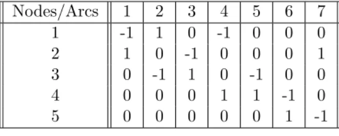
4.1 Network Used in the Illustration . . . 46
4.1 Node-Arc Incidence Matrix . . . 45
4.2 Demand Estimates . . . 46
4.3 Routing Costs . . . 47
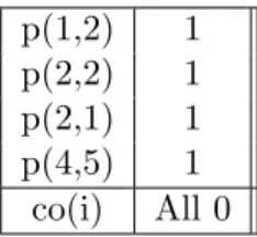
4.4 Optimal Values of the Coefficients . . . 51
4.5 Routings with AARC and ARC . . . 52
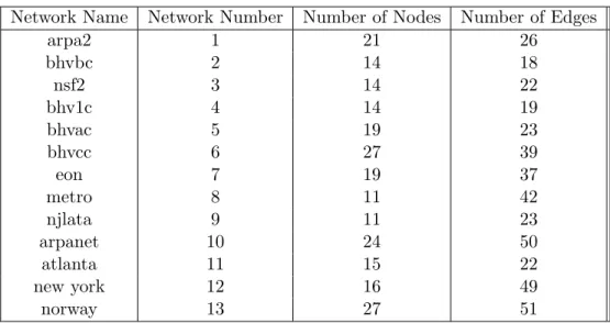
5.1 Properties of the Networks . . . 53
5.2 Results-Main Model . . . 57
5.3 Results-Extension 1 . . . 58
5.4 Percent Losses of RC and AARC with Main Model and Extension 1 59 5.5 Increase in Percent Losses of RC and AARC with Main Model and Extension 1 . . . 59
5.6 Relative Percent Improvement of the AARC against RC . . . 60
5.7 Results-Extension 2 . . . 60
5.8 Simulation Results-Main Model-Budget=1000 . . . 63
5.9 Simulation Results-Main Model-Budget=3000 . . . 64 ix
5.10 Simulation Results-Main Model-Budget=10000 . . . 65
5.11 Simulation Results-Extension 1-Budget=1000 . . . 68
5.12 Simulation Results-Extension 1-Budget=3000 . . . 69
5.13 Simulation Results-Extension 1-Budget=10000 . . . 70
5.14 Simulation Results-Extension 2-Budget=1000 . . . 71
5.15 Simulation Results-Extension 2-Budget=3000 . . . 72
Introduction
1.1
Uncertain Optimization Problems and
Deal-ing With Uncertainty
Robust optimization has been one of the most interesting branches of the combi-natorial optimization literature that have emerged over the past twenty to thirty years. The theory of robustness deals with uncertainty of problem parameters. It is a fact that an amount of uncertainty in parameters always exists due to the nature of real world problems. For example, for the network design case, uncer-tainty in problem parameters may come from many reasons such as breakdown of a link in the network, uncertainty in the routing or capacity installation costs, nature and human factors, uncertainty of supply or demand, etc. Therefore it appears to be important to identify classes of models in which small changes in problem data lead to small changes in the result under the worst plausible sce-nario. It can be said that the interest for robust models has been a consequence of the need for formulations that by design yield solutions that are less sensitive to the input data than classical formulations.
As mentioned before, in real life data are always subject to change and it is very hard (if it is not impossible) to obtain exact data related to any system.
Additionally, even if exact data can be obtained, sometimes the optimal solu-tions found after modeling cannot be applied due to some constraints in real life. This fact can also be considered with the use of some uncertain data during the modeling process. Optimization problems that arise from these uncertain data are called uncertain optimization problems. The uncertainty may be related to the objective function coefficients, the coefficients of some or all of the variables in the constraints, the right hand sides of the constraints, etc.
In operations research, there exist different ways to cope with uncertainty. One approach can be to ignore uncertainty throughout the optimization process. The model is developed and solved with the use of some nominal data (perhaps most likely values obtained via estimates). Afterwards Sensitivity Analysis is used as a post-optimization tool to give an idea about the affects of uncertainty (introduced in terms of small disturbances) against the optimal solution found via nominal data. Here sensitivity analysis is used to test the stability of the nominal solutions against uncertainty but it does not help to obtain solutions that are stable. In Stochastic Programming, uncertainty is handled from the beginning of the model development stage of the process. In order to apply this approach, one needs information about the underlying probability distributions that describe the uncertainty of the parameters. In real life applications, this is often very hard which causes difficulties in using this approach. One other approach is Scenario Based Robust Programming. In this approach, uncertainty is represented with the use of several different scenarios. A solution, which optimizes a criterion among these scenarios, is sought. An important problem about this approach is that the size of the resulting model gets very large as the number of scenarios increases.
As mentioned above, sensitivity analysis is a post-optimization tool and can-not be used to find a robust solution. On the other hand, in stochastic program-ming and scenario based robust programprogram-ming approaches, a solution obtained is allowed to be infeasible for some realizations of the uncertain data or some of the scenarios. In most cases, violated constraints are taken into account by adding some penalty to the objective. In real life, there exist applications in areas such as engineering, pharmacology, physics, chemistry, etc. in which even a minor violation of the constraints cannot be tolerated. Under the existence of such
constraints, the approaches of stochastic programming and scenario-based robust programming are not applicable since they allow violation of the constraints un-der uncertainty. Therefore, there exists a need for an approach that does not allow any violation of the constraints. Robust Counterpart (RC) approach is the answer to this need.
Under RC approach, there exist hard constraints which cannot be violated under any condition therefore results that are feasible for all realizations of the uncertainty are obtained. Depending on the structure and hardness of the prob-lem, extensions of the RC model namely Adjustable Robust Counterpart (ARC) and Affinely Adjustable Robust Counterpart (AARC) are developed and used in the literature. Detailed information about these concepts will be presented in Chapter 3.
1.2
Brief Contents of the Study
In this thesis, we consider the capacity expansion-routing problem. In particular, we are given a capacity budget and asked for how to use this budget in order to minimize the overall routing cost in the network. One important assumption is that we can find a feasible solution (i.e. a feasible routing) for every realization that can come out of the uncertainty set. Therefore we do not try to convert an initially infeasible problem to a feasible one by installing additional capacity to edges. Our problem is to find the best allocation of the capacity budget to edges in the network in order to minimize the routing cost under uncertain demand.
We define a robust solution as the one that minimizes the worst-case cost under demand uncertainty. Therefore the solution obtained should be feasible for any realization coming out of the uncertainty set and in addition it should be the one with the cheapest cost among such solutions.
In each network, there is a single source node and multiple demand nodes as well as transshipment nodes. The demand is uncertain. The uncertainty is modeled as follows. We assume that, we have an average demand value for each
demand node and we use these averages as demand estimates for the demand nodes. These estimates can vary in both directions with a constant percent error for all the demand nodes. On the other hand we can supply all the demand from the single source for any realization of the uncertainty. This means that there is no constraint on the supply amount. In addition there are coupling constraints that couple the demands of the two nodes, which imply that if a demand value more than the estimate is observed at one node than the demand value observed at the coupling node should be less than its corresponding estimate. Initial capacities on the edges of the network and routing costs are known and deterministic.
Having described the basic model, we consider three different versions of the model in this thesis. In the first model, the capacity can be installed in continuous amounts, that is to say there exists no integrality restrictions. In the second model, we introduce modular capacity into the model. We have links with a fixed capacity and can install integer amount of links on the edges in order to increase the capacity. The capacity constraint is expressed in terms of number of links that can be installed in this case. The third model is an extension to the second. In addition to the second model; we introduce fixed and variable capacity installation costs to our objective function. For each model, we generate instances with low, medium and high uncertainty and capacity budgets.
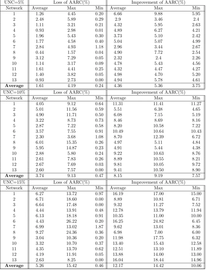
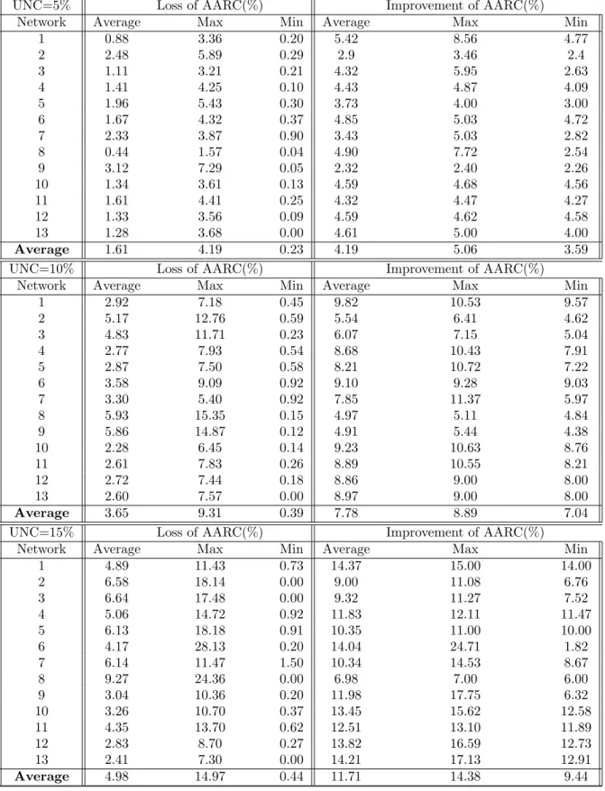
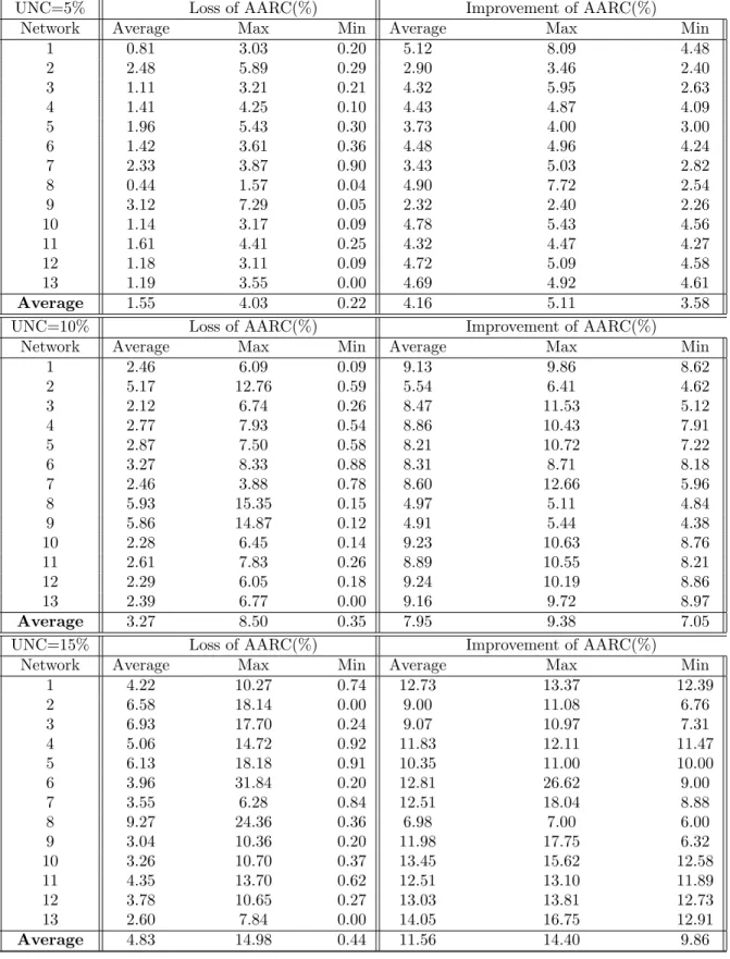
The results are reported through two studies in the experimental part. In the first study we generate different problem instances on each network and evaluate the average performance of the AARC optimal solution (i.e. an approximation to the worst-case cost of the ARC) against the RC optimal solution and the optimal solution of the basic model using deterministic nominal data (i.e. estimates of the demand). Second experiment is a simulation study. A problem instance from the first experiment is fixed for each network topology and 2000 random demand vectors are created from the uncertainty set. Afterwards the costs of the AARC and RC solutions are calculated for each demand vector and to evaluate the costs of these solutions, they are compared with the cost coming from the deterministic solution.
definitions and formulations of the concepts of RC, ARC and AARC. Next, in Chapter 3, a review of the literature on general robust optimization as well as the robust network design in particular are presented. In the following chapter, the model used in the thesis as well as the corresponding RC, ARC and AARC formulations are given. In addition, a small network example is provided in order to illustrate the formulations. The chapter also includes two propositions that show the equivalence of RC, ARC and AARC under two different uncertainty sets. Chapter 5 deals with the detailed results of the experimental study as well as their interpretation. We conclude in Chapter 6.
General Definitions and
Formulations
A general linear programming (LP) problem is formulated as:
Min{ctx : Ax ≥ b}. (2.1)
When uncertainty in parameters is introduced into the system, we are faced with an uncertain linear programming problem. An uncertain linear programming problem is defined as a family of instances as formulated below where U ⊂ Rn∗
Rm∗n∗ Rm is defined as the uncertainty set.
Min{ctx : Ax ≥ b} where (c, A, b) ∈ U. (2.2)
In robust optimization methodology, the notion of robust counterpart (RC) of a problem tries to find an optimal solution to an uncertain LP under the condition that the solution obtained is feasible for all the realizations of the data coming from a known uncertainty set. Such solutions are defined as uncertainty-immunized solutions in [2]. It can be said that the optimal solution of the RC is the one that gives the best objective function value among the solutions that are
feasible for all realizations of the uncertainty.
The robust counterpart problem is formulated as follows:
Min{ctx : ∃x : Ax ≥ b ∀(c, A, b) ∈ U} (2.3)
Note that we assume there exists a feasible solution (i.e. the problem is not infeasible).
While solving the robust counterpart of a problem, one important fact is the following: The decisions about all the variables in the problem should be given at one stage. This means that the problem should be solved and an optimal solution should be found in one shot. All decisions about the variables should be taken before the actual realization of the data. But there are cases in which some of the variables are decided prior to the realization of the uncertainty and some of them can be decided after the realization. An example is the capacity expansion-routing problem. The decision maker should decide how to allocate the capacity budget to the existing edges before the actual realization of the uncertainty but the routing decisions can be given after realizing the actual values of the uncertain parameters.
In [2], the notion of Adjustable Robust Counterpart (ARC) is introduced to deal with these types of problems. The variables in the problem are divided into two groups as adjustable and non-adjustable variables. Non-adjustable variables are the ones that are decided prior to the realization of the uncertainty and the adjustable variables are the ones that can be adapted to the actual realization of the data. The benefit of the ARC over the classical RC is that in some cases, the RC provides solutions that are unjustifiably conservative resulting in high costs in terms of objective function value.
If we divide the variable vector −→x into two (i.e. divide the variables into two groups) as the adjustable variable component −→y and non-adjustable variable component −→z , we can formulate the adjustable robust counterpart problem as:
Minz{ctz : ∀(c, A, b) ∈ U ∃ y(c, A, b) : By + Cz ≥ b} (2.4)
Note that, the matrix A is divided into two parts as B and C that correspond to adjustable and non-adjustable variable coefficients. With this notation, the formulation of RC becomes:
Minz{ctz : ∃y such that ∀(c, A, b) ∈ U : By + Cz ≥ b} (2.5)
Although the formulations given by (2.4) and (2.5) look similar, there exists a significant difference. In RC formulation, we are given the uncertainty set and we want to be sure that there exists a solution that is feasible for every realization that can come out of the uncertainty set. In this formulation, having adjustable variables does not bring any advantage. On the other hand, in ARC formulation, given any point from the uncertainty set, we want to optimize over all values of the non-adjustable variables for which there exists a feasible adjustable variable component. This means that the solution vector (i.e. the adjustable part of the solution vector) can be adjusted after the realization of the uncertain data in ARC. Therefore the feasible set of ARC is larger than that of RC which results in a less conservative solution.
Although ARC is far less conservative when compared with the RC, it is known that the ARC problem is computationally tractable for only a limited number of cases (see [2] for details). As a result, a need for an approximation of ARC has emerged. In [2], the notion of Affinely Adjustable Robust Counterpart (AARC) (see also [21]) is introduced. In AARC, the second-stage variables (i.e. adjustable variables) are restricted to be affine functions of the uncertain parameters. In fact, the dependency between the second stage variables and the uncertain parameters can be expressed via several functional forms. The affine dependency used in the AARC approach results in computationally tractable problems and therefore it is preferred against the others. With the restriction imposed by the AARC approach, only an approximation to the ARC is calculated. On the other hand tractability of the problem is significantly improved. The affinely adjustable
robust counterpart problem is formulated as:
Min(z,w,W ){ctz : B[w + W β] + Cz ≥ b ∀(c, A, b) ∈ U} (2.6)
Note that in the above formulation, we set y = w + W β where β ∼= [c, A, b] ∈ U, therefore we replace the adjustable variables y by an affine function of the uncertain parameters. In the AARC formulation, if one sets the variable W to zero, then the obtained formulation is equivalent to that of RC. As mentioned before, AARC is an approximation to ARC and it is in between ARC and RC in terms of conservativeness.
Literature Survey
Although robust optimization is a relatively new area of operations research, there exists a substantial amount of work worth mentioning in the literature. In this thesis, we consider robust network design but ideas developed in robust optimization are applied in a wide range of areas such as scheduling, inventory control, etc.
In this chapter, literature on robust network design as well as the benchmark papers related to general robust optimization methodology will be summarized. The papers by Ben-Tal and Nemirovski ([2], [3], [4], [5], [22] and [23]) are worth to be mentioned since they contribute a lot to the robust optimization theory. The concepts of ARC and AARC are first mentioned by these authors. Papers by Ordonez et. al. ([19] and [21]) as well as the paper by Atamt¨urk and Zhang [1] can be seen as the source of the models developed and tested in this thesis. In the mentioned papers the concept of ARC is investigated in detail.
Bertsimas and Sim ([6], [8] and [9]) are also among the authors who concen-trate on robust optimization. Yaman, Kara¸san and Pınar ([13], [24] and [25]) as well as Kennington et al.([11] and [12]) are among the important sources in appli-cations such as robust spanning trees, robust shortest paths and robust DWDM routing.
Below, detailed summaries of the mentioned papers as well as some other important sources are given. To improve the flow of the presentation, the papers related to each other are summarized one after another.
Ben-Tal, Goryashko, Guslitzer and Nemirovski [2] work on the type of prob-lems which include uncertain parameters lying in a predefined uncertainty set and in which some of the variables must be determined before the realization of the uncertainty while the others can be adjusted after the realization of the un-certain parameters. The former ones are defined as non-adjustable variables and the latter ones as adjustable variables. Using these definitions, the notion of “Ad-justable Robust Counterpart” (ARC) is introduced. The ARC of an uncertain LP is less conservative than its robust counterpart (RC) which simply minimizes the guaranteed value of objective of an uncertain LP while staying feasible under all realizations of the uncertainty set.
After formulating the ARC, the cases where the ARC of a problem is equiva-lent to its RC are investigated. It turns out that the cases where the uncertainty affecting every one of the constraints is independent of the uncertainty affect-ing all other constraints are the ones in which RC and ARC of a problem are equivalent. Furthermore, it is shown that even in simple situations when two or more constraints can depend on the same uncertain parameter, the ARC can significantly improve the solution given by RC. Next it is mentioned that the ARC is not computationally tractable in many cases and because of this fact the “Affinely Adjustable Robust Counterpart” (AARC) of a problem is introduced. It is an approximation to the ARC in which there exists a restriction on how the adjustable variables are tuned to the data. The main idea is to require the adjustable variables to be affine functions of the data. Afterwards, the authors show that the AARC is computationally tractable in many cases in which ARC is NP-Hard.
Next, a tight computationally tractable approximation applicable to many cases is developed. The AARC approach is illustrated by considering an inventory management problem. It was found out that the price paid in terms of objective function value in exchange for robustness is surprisingly low.
Ordonez and Zhao [19] consider a transit network and present a capacity ex-pansion method that is robust against uncertainties in travel times and demands. They mention that investments in highway infrastructure are constantly under-taken and the methods developed in the paper can be useful to give profitable investment decisions. They define the robust solution as the solution that achieves the best worst-case objective function value. The authors also talk about robust counterpart and adjustable robust counterpart problems. Robust counterpart of a problem simply tries to minimize the objective value considering all instances that can come out of the uncertainty set. Consequently the objective is minimiz-ing the worst-case cost. The RC problem for a stochastic problem with recourse leads to the adjustable robust counterpart problem (ARC). In an ARC problem, some of the decision variables are decided a priori and the rest can adjust to the outcome of the uncertainty. It is a fact that optimal objective value of the ARC formulation (zARC) is less than or equal to optimal objective value of RC
formulation (zRC) [see [19] for details].
The problem considered in the paper is represented by a transportation net-work using a classic netnet-work flow formulation where the flow is routed by the system to minimize the total travel time. Each arc in the network has an initial fixed capacity and this capacity can be expanded by using a budget. There exists a limited budget and the question to answer is how to allocate this limited budget under uncertainty in demands and travel times while satisfying the demand at each node. Given uncertainties in demands and travel times, one can separate the decision variables by deciding capacity expansion variables prior to observation of the demand and have the traffic flow adapt to the demand while minimizing total travel time. This means that the robust capacity expansion problem (RCEP) is an example of ARC problem.
After mentioning the above fact, it was shown that the RCEP problem could be expressed in a simpler form, which can be seen as a model, which minimizes the maximum possible cost (i.e. worst case cost). One important assumption (Assumption 1) in the paper is that the uncertainty sets are closed, convex and bounded. In addition, the considered network is feasible for every instance that can come out of the uncertainty set even if the budget is zero (i.e. a feasible flow
can also be found without installing any capacity other than the initial capacity on arcs). This means that the budget capacity will be used to improve the objective function not to convert an initially infeasible network design to a feasible one.
Next, the worst case cost of investment decision y called Θ(y) is defined and it was shown that under Assumption 1, Θ(y) is a convex function in y. Therefore RCEP is the minimization of a convex function over a simplex and it can be NP-Hard only when evaluating Θ(y) cannot be done in polynomial time. Afterwards two simple examples showing that finding the worst-case demand combination can indeed be a difficult problem are presented.
The authors also present the cases in which tractable solutions for RCEP can be obtained. The first case is the case of deterministic demand. Under determin-istic demand they give a robust counterpart formulation (RC), which was shown to be tractable for the considered uncertainty sets. The authors show that RCEP is equivalent to RC problem under certain demand and the mentioned uncertainty in travel times and therefore RCEP is also tractable. The second tractable case is the case of uncertain demand. In this case, the conditions on the uncertainty set under which Θ(y) can be evaluated efficiently, were determined. It was shown that RCEP is tractable when there exist multiple sinks and a single source or equivalently multiple sources and a single sink, with demand uncertainty only in a single source and sink pair. Under these cases, Θ(y) was shown to be a con-vex optimization problem. With demand uncertainty sets defined as above, the case of different traveling time uncertainties were investigated. The final case, in which RCEP is tractable, is a multi-commodity flow problem with a single source (or sink) per commodity and uncertainty only on a single source-sink pair per commodity. Once more it was shown that, Θ(y) is a convex optimization prob-lem under mentioned conditions and fairly general uncertainty sets representing travel times.
In the computational experiments part, the optimal value of the determin-istic solution, the optimal value of the robust solution, the worst-case value of the deterministic solution and the objective value of the robust solution for the nominal data were calculated. The results indicate that the robust solution can
reduce the worst case cost by more than 20% while incurring in about a 5% loss of optimality with respect to the optimal deterministic solution for a nominal un-certainty data. It is concluded that the robust solution becomes more attractive as the uncertainty in travel times increases and as the budget to decide capacity expansions increases. In addition the greatest benefit of a robust solution is ob-tained for flow in some medium range, as a network with small amounts of flow is not affected by capacity expansions and a network with large amounts of flow is forced to send flow through less attractive routes.
Mudchanatongsuk, Ordonez and Liu [21] present a robust optimization based formulation for the network design problem under transportation cost and de-mand uncertainty. The considered problem and the ideas developed are exten-sions of the ones developed in [19]. They work on the topic of network design in order to make decisions on where to increase arc capacities to reduce the overall network routing/transmission cost.
In the paper, a classic multi-commodity network design problem (NDP) is considered. The aim is to find out the arcs on which capacity will be installed in order to minimize the total routing cost and the capacity installation cost. The problem is formulated as MIP. The authors assume that the network problem is always feasible even if no capacity is installed on the arcs. This is provided by installing incapacitated, high-cost, artificial arcs between all source and sink nodes for each commodity. As in [2], the robust solution is defined as the solution that has the best objective value in its worst-case uncertainty scenario.
The robust counterpart (RC) and the adjustable robust counterpart (ARC) concepts are mentioned as in [19]. The network design problem has a natural separation between “here and now” decisions and “wait and see” decisions. This implies that, investment decisions are made before observing the demand and the routing decisions are made according to actual demand observations. In the study, the uncertainty sets are defined as deviations from an estimated or nominal value of the uncertain parameter. It is mentioned that the sets used are quite general and can represent arbitrary correlation structures in the uncertain parameters. Since ARC is hard to solve in general the solution approach introduced in [2]
is used. The approach approximates the problem by limiting the second stage variables to be some affine functions of the uncertain parameters. At this stage one key assumption of the authors that leads to an important simplification is that, each commodity has a single source and a sink.
The authors prove that, their selection of the affine function of the second stage variables guarantee to solve the approximate problem efficiently. After-wards, the efficiency of the approximation to the adjusted robust counterpart problem obtained by limiting the recourse variables to affine functions of uncer-tain parameters is investigated. One important note is that for affine functions of the uncertain parameters the optimal objective value of the affinely adjustable robust counterpart (AARC) is in between the optimal objective value of the ro-bust counterpart (RC) and the optimal objective value of the adjustable roro-bust counterpart (ARC). Next, the authors show that for the NDP with single sink and single source for each commodity and non-negative costs for each arc, the AARC of the arc-flow formulation is equivalent to the RC of the path-flow formulation. The authors also develop the path variable based formulation of the problem and a column generation procedure that is appropriate for the linear relaxation of a path constrained robust network design problem. Solving the linear relaxation efficiently leads toward lower bounds and the algorithms for the integer RNDP.
After numerical analysis, the authors conclude that the AARC which is an approximation to ARC and even its LP relaxation has modest sub-optimality on any specific deterministic scenario while significantly reducing the worst-case cost, in particular as the uncertainty increases. In addition, the simulation studies show that the approximate robust solution reduces the mean and standard deviation of the total cost, in particular for large problems.
Atamt¨urk and Zhang [1] describe a two-stage robust optimization approach for solving network flow and design problems with demand uncertainty. In the considered types of problems, typically, design and capacity allocation decisions are made at the first stage and routing decisions are made at the second stage after the realization of the uncertain demand. They focus on two-stage network flow and design and characterize the set of robust first stage decisions explicitly
by exploiting the underlying network structure.
They define the robust first-stage decision set, P(A), as the set of first-stage decisions for which there exists some feasible second-stage decision for all real-izations of the uncertain demand. Similarly Q(A) is defined as the set of robust first-stage decisions when integer design variables are introduced into the model. Two types of uncertainty sets (budget uncertainty set and cardinality-restricted uncertainty set) are considered. It is shown that the separation problem for P(A) is NP-Hard for both uncertainty sets and bipartite graphs and the separation problem for Q(A) is NP-Hard for both uncertainty sets. The authors also show that by using a budget of uncertainty for demand, it is possible to give an up-per bound on the probability of infeasibility of the robust solution for a random demand vector. Next some computationally tractable cases (namely totally or-dered graphs, arborescence and examples from production lot-sizing problems) are considered. Extensions to multi-commodity cases are considered in two cases namely arc-based stages and commodity-based stages.
In the computational analysis part, two-stage robust optimization framework is applied to the facility location problem with uncertain demand. The experi-ments indicate that the proposed approach provides an interesting trade-off be-tween scenario based stochastic programming and the conservative single-stage robust optimization.
Ben Tal and Nemirovski [22] study convex optimization problems for which the data is not specified exactly but known to belong to a given uncertainty set. In addition the constraints must hold for all possible realizations of the data. In order to address the uncertainty, the approach of robust counterpart [RC] is utilized as in [3] and [8]. The primary goal for application of the robust optimization approach is converting the robust counterparts of generic convex problems to explicit convex optimization problems accessible for optimization algorithms. In the paper, it is shown that in several important cases such as linear programming, the use of ellipsoidal uncertainties leads to explicit robust counterparts, which can be solved both theoretically and in practice. The mentioned explicit forms are tried to be derived for general uncertain optimization problems in the paper.
The main questions answered are: If all instances of an uncertain program are solvable,
• Under what conditions, is RC solvable?
• When is there no gap between the optimal value of the RC and the worst of the optimal values of the instances?
• What can be said about the proximity of the robust optimal value and the optimal value in a nominal instance?
Ben Tal and Nemirovski [3] consider linear programming problems with un-certain data, which include hard constraints that must be satisfied whatever is the actual realization of the data (as in [22]). They give a definition of the robust counterpart (RC) of an LP program and give the assumptions (see [3] for details) that are necessary to guarantee the following:
• The RC of an LP is infeasible if and only if there exists an infeasible instance of the original LP
• The optimal value of the RC is equal to the maximum optimal value among the all possible scenarios of the original LP
Next, they work on the geometries of the uncertainty set which lead to a computationally tractable RC. They focus on the geometries leading to explicit RC of nice analytical structure and which can be solved by high-performance optimization algorithms. They prefer a structure where the uncertainty set is an intersection of finitely many ellipsoids. For this case, the explicit form of the RC is developed and it turns out to be a conic-quadratic problem. The robust solution is illustrated with a simple portfolio selection example.
Ben-Tal and Nemirovski [4] perform an experimental analysis on the effects of uncertainties in the coefficients of the variables in the constraints of an LP. Their claim is that, in real life applications, coefficients of the variables cannot be estimated very accurately and when looked from a practical point of view an
optimal solution to an LP can be severely infeasible if the nominal data is slightly perturbed.
In the experiment, they work on 90 LPs from the well-known NETLIB collec-tion and calculate a reliability index in order to measure the robustness (in terms of feasibility) of each nominal solution against perturbations in the coefficients of the variables in the constraints. The result is that in about 50% of the instances, the nominal solution can easily be infeasible in case of small perturbations.
Next, the authors develop a strategy to find out robust solutions. Two types of uncertainty cases are considered. The first one is “unknown but bounded uncertainty” and the second one is “random symmetric uncertainty”. In the first one the nominal solution is expected to satisfy the constraints with a maximum error of a specified value (*). To find out such a solution, an interval robust counterpart problem is solved (a variation of the RC problem defined in [2]). In the second one, uncertain coefficients are obtained by random perturbations that are independent random variables within a predefined interval. In this situation, the deterministic requirement (*) is changed with a probabilistic version.
The experimental analysis shows that when passing from a usual optimal solution to a reliable one, one does not necessarily lose a lot from optimality. In addition, in many cases, a robust solution cannot be obtained by a moderately small correction of the nominal solution, which implies that the methodology presented in the paper is essential.
Ben-Tal and Nemirovski [23] work on the methodology and applications of robust optimization. They consider linear, conic quadratic and semi definite programming problems with an uncertainty set that consists of an intersection of ellipsoids. They mention that RC of an uncertain LP is equivalent to an explicit computationally tractable problem if uncertainty set itself is also computationally tractable (see [3]). As an illustration of RC approach, they give an example about antenna design. They also mention the study conducted in [4]. Next the authors talk about robust quadratic programming and mention that even with a simple uncertainty set the RC can become an NP-Hard problem in contrast to linear programming (see [22]). Therefore they concentrate on approximations to the
RC problem. This approach is also illustrated with an example of antenna design problem. Finally, robust semi definite programming is considered. The cases in which RC is tractable are investigated and an approximation is developed for the cases which are not tractable.
Ben Tal, Nemirovski and Roos [5] consider a conic-quadratic optimization problem with uncertain data lying in some uncertainty set. When RC approach ([4], [9], [22] and [23]) is applied to such a problem, it is mentioned that it usually leads to an NP-Hard semi definite problem. An example is the case when uncertainty set is an intersection of ellipsoids. For the mentioned NP-Hard cases a simple, explicit semi-definite program is developed which approximates the RC. In addition, an estimate of the quality of the approximation is derived.
Laguna [16] works on the problem of expanding the capacity of a single fa-cility in telecommunications network. It is mentioned that capacity expansion problems in telecommunications have changed in nature due to the emergence of new technology. Different options to increase the capacity of a network are of-fered and this brings the problem of which option to choose. Simply the problem under consideration consists of finding the combination of components (each with a different price and capacity) that should be installed in each period in order to meet a total demand at a minimum discounted cost.
The key idea used in the paper to find robust solutions is to define a collection of plausible model representations as a set of scenarios. The resulting large-scale optimization problem introduces a new objective to ensure that the model recommendations are close to optimal regardless of which scenario occurs. The problem is solved in two phases. In the first phase a dynamic programming recursion is solved and in the second phase a shortest path procedure is applied. After numerical experiments it was found out that a large number of scenarios could be handled with the developed technique since the computation times are more sensitive to the maximum demand across all scenarios than to the number of scenarios considered.
Riis and Andersen [17] consider a capacity expansion problem in a telecom-munications network with uncertain demand. The problem is to install additional
capacity on the edges of a network and route traffic while minimizing the rout-ing costs and satisfyrout-ing the demand. The capacity installation can be performed through the usage of two types of facilities. In the paper, first, a formulation of the deterministic capacitated network design problem is presented and some well-known valid inequalities are mentioned. Then the problem is formulated as a two-stage stochastic problem with integer first stage and continuous second stage variables. As in [1], [2], [19] and [21], the variables are grouped into two as first stage (where and how much capacity to install) and second stage (routing decisions) variables. Next the valid inequalities for the deterministic case are investigated in order to adapt them to the new formulation. A heuristic based solution procedure that makes use of these inequalities is developed.
The developed algorithm is tested using two sets of real life data through the generation of scenarios. The developed method is found as a practical tool for network design in real-life applications.
Riis and Andersen [18] work on the same problem as Laguna [16] (multiperiod capacity expansion of a telecommunications connection with uncertain demand). The problem is to determine the number and type of facilities to install at each period to satisfy the demand which is uncertain. The uncertainty in demand is modeled in terms of scenarios that represent different outcomes of random demand. Two different models are developed. The first model introduces a simple preprocessing rule that reduces the computation time of the two-stage algorithm developed in [16]. In contrast to the two-stage approach developed in [16], a multistage solution procedure is developed in the second model which is viewed as a more accurate description of the system by the authors. The experiments show that the second model is practical but needs much more time than the two-stage approach.
Betsimas and Sim [8] develop an approach to address data uncertainty for discrete optimization and network flow problems. They consider mixed integer programming problems and assume (w.l.o.g.) that the uncertainty only affects the objective function coefficients and the coefficients of the constraint matrix. Each entry in the constraint matrix is modeled as an independent, symmetric and
bounded random variable with an unknown distribution. Each cost coefficient is modeled as variables that have deviations from a nominal value. In order to control the degree of conservatism of the solution a parameter is introduced for each constraint (τ ) that defines the maximum number of coefficients that are allowed to deviate in the problem. Therefore it is assumed that only a subset of the coefficients will change in order to adversely affect the solution. The authors are interested in finding an optimal solution that optimizes against all scenarios under which a maximum number of τ coefficients can vary in order to maximally influence the objective. Next the proposed robust counterpart (RC) formulation and an equivalent MIP formulation is presented. It is shown that even if more than τ coefficients are subject to change, the RC solution will still be feasible with a very high probability.
Afterwards robust combinatorial optimization problems are considered. An algorithm, which shows that the RC of a polynomially solvable combinatorial optimization problem is also polynomially solvable, is presented. It is shown that when only cost coefficients are subject to uncertainty in a polynomially solvable 0-1 discrete optimization problem, the RC also remains polynomially solvable. The authors also deal with robust approximation algorithms and finally they give an algorithm for robust network flows that solves the RC by solving a polynomial number of nominal minimum cost flow problems in a modified network.
In the experimental study, robust knapsack, robust sorting and robust shortest path problems are considered. The approach was found practically useful espe-cially for combinatorial optimization and network flow problems that are subject to cost uncertainty.
Bertsimas, Pachamanova and Sim [6] develop a method for robust modeling of linear programming problems using uncertainty sets described by an arbitrary norm. In the paper, robust counterparts of the linear programming problems arising from uncertainty sets given by different forms are characterized. In addi-tion, probabilistic guarantees on the feasibility of an optimal robust solution are investigated.
they call as the price of robustness. This study can be considered as an extension to [8]. They mention the fact that robust optimization methods usually result in very conservative solutions with objective values far away from the optimal. Therefore efficient methods that can control the conservatism of the robust so-lution are needed. They define a parameter related to the maximum number of coefficients allowed to change in a model. With the help of this parameter, the conservatism of the solution is kept under control. They find solutions that stay feasible if no more than the assumed number of parameters are allowed to be uncertain (controlled by the parameter). In addition, they show that the prob-ability of the found robust solution to stay feasible in the presence of uncertain variables more than the assumed value is very high. The developed method pro-poses a robust formulation that is linear and thus it can be extended to discrete optimization problems easily.
Yaman, Kara¸san and Pınar [25] concentrate on the robust version of the mini-mum spanning tree problem. In the considered networks, edge costs are specified as interval numbers which are independent of each other. Two types of robustness are considered. A spanning tree with a minimum absolute worst case scenario (i.e. costs of all the edges in the spanning tree are at their upper bounds) is called an absolute robust spanning tree and it is shown that such a tree can be found in polynomial time. Secondly, a spanning tree whose total cost minimizes the max-imum deviation from the optimal spanning tree over all edge cost realizations is called a relative robust spanning tree. MIP formulation is given to find such a tree. They define concepts such as weak edge and strong edge which are used to preprocess the graph efficiently. This preprocessing makes it easier to solve the MIP formulation developed by the authors.
Yaman, Kara¸san and Pınar [24] work on the robust shortest path problem. They consider directed acyclic graphs and arc lengths that are uncertain parame-ters represented as interval numbers. As in [25] a min-max regret criterion is used to find a robust solution. MIP formulation is provided for the problem. Arcs in the networks are classified into groups. With the help of this classification arcs that cannot be on a shortest path for any realization of the uncertain parame-ters are determined. This preprocessing makes it easier to solve the considered
problems.
Kennington et al. [11] develop a new set of models for the dense wave-length division-multiplexing (DWDM) problem that combine methods of pro-tection against a single link failure and robust design strategies. The target is to find the optimal routing for each demand (given a forecast for each) and to determine the optimal amounts of equipment to be loaded on the links of the net-work. Three different protection strategies against failure of a single link, in case where point-to-point demand is known with certainty, are mentioned. Unknown demands are taken into account using a discrete probability distribution with a sample space. Each sample space realization represents a scenario with a corre-sponding probability. A regret function is used to model robustness, which prefers solutions that work reasonably well under every scenario considered. Models that are combinations of the protection strategies against link failures and robust op-timization approach are developed.
Kennington et al. [12] consider a dense wavelength division-multiplexing (DWDM) network. They have estimates of the point-to-point demand in the network and the problem is to determine the routing for each demand and the least cost capacity installation that will support this routing as in [11]. The de-mand in the network is uncertain and the forecasts are not reliable. Therefore they use scenarios to represent the uncertainty. The authors want to develop a robust solution that will work well under all the scenarios considered. A regret function is used to find robust solutions. Regret is realized in two ways. The first way is the installation of capacity that is not utilized fully when demand is realized. The second way is installation of less capacity than needed so that some of the demand cannot be satisfied by the system. A second objective other than the robustness is the cost of the network design (i.e. cost of the equipment installed). Therefore the authors develop a multicriteria model to take both ob-jectives into account. A two-phase optimization strategy is developed. In the first phase a robust solution that minimizes the regret is found but there exists a budget constraint. In the second phase regret is fixed to the optimal value found in the first stage and a minimum cost solution is searched under this constraint.
Another work on DWDM routing and provisioning at minimal cost belongs to Kara¸san, Pınar and Yaman [13]. Different from [12], they use a flow based formulation instead of path formulation and investigate uncertainty models based on polyhedral representations of the uncertain demands instead of scenario based representations. The authors consider both targets of robustness and network de-sign cost in one single model in contrast to the two-phase model in [12]. Two mod-els of polyhedral uncertainty (namely hose model and restricted interval model) are used and MIP formulations of the corresponding robust problem as well as valid inequalities are provided.
El Ghaoui and Lebret [15] work on least-square problems with uncertain but bounded coefficient matrices. They provide an algorithm to minimize worst-case residual error using second-order cone programming. Methods on how to mini-mize upper bounds for the optimal value of the worst-case residual for different perturbation vectors on data are developed.
El Ghaoui, Oustry and Lebret [10] consider semi-definite programs in which data is uncertain due to bounded deterministic perturbations. They look for a ro-bust solution that remains feasible for all data and that minimizes the worst-case cost. Sufficient conditions for semi-definite programs to guarantee the existence of robust solutions are mentioned. In addition conditions under which there ex-ists a unique robust solution are searched in detail. Results are illustrated using examples taken from linear programming, integer programming, etc.
Kouvelis and Yu [14] present a comprehensive study that includes detailed information about the techniques used in discrete optimization concerning ro-bustness as well as different references about the topic. Most of the results given in the book correspond to scenario-based modeling of the uncertainty, which consists of a finite number of scenarios that correspond to different realizations from the uncertainty set. With scenario based-uncertainty, the authors show that most solvable combinatorial optimization problems turn out to be NP-Hard when robustness is considered.
In this thesis, we concentrate on a capacitated network design problem. The considered model is the same as the one developed in [19]. Unlike [19] which
considers both demand (i.e. righthand side) and cost(i.e. objective function coefficient) uncertainty, we consider only demand uncertainty in our study. In [19], the model is tested for the cases (i.e. uncertainty sets) in which ARC can be solved efficiently. Therefore there exists no need for the application of AARC approach. We show that for the uncertainty set considered in [19] for which the ARC can be solved efficiently, AARC, RC and ARC approaches are all equivalent. Next, in our main study, we consider an uncertainty set for which the ARC model cannot be solved efficiently. Therefore we apply the AARC approach introduced in [2] to our model in order to find an approximation to ARC. We also solve the RC of the same problem and compare the results obtained from RC and AARC against the results obtained by solving the model via nominal certain data (i.e. estimates of the data). Results of a comprehensive simulation study are also presented in the second part of the experimentation study. The concept of AARC is also applied by Ordonez et al. to a similar problem in a recent study ([21]). In that study, only a single model is under consideration and the capacity budget constraint is omitted. In addition the decision to give is whether to install a pre-specified amount of capacity to an edge or not which is decided by the use of binary variables. In other words, the decision maker is not allowed to install any value to an edge. In our study there exist three different extensions of the model and all of the extensions include a capacity budget constraint. In the first extension, any value of capacity can be installed on any edge and there exist no integrality restrictions. In the second extension, modular capacity concept is introduced and links with a certain capacity can be installed on edges in integer amounts. In the last extension, modular capacity approach is again used but this time with fixed and variable capacity installation costs in the objective function. As far as we know, this study is one of the rare works that concentrate on the AARC approach developed recently. In addition, it is the first study that compares a single stage robust solution (RC) with a double stage one (AARC) in network design.
Problem Formulation
In this thesis, we work on a robust capacity expansion-routing problem. Given a network, we have a single source node, transshipment nodes and demand nodes. The demand of the nodes is uncertain but known to belong to a well-defined uncertainty set. We are given a capacity budget and we try to determine the best allocation of the given capacity budget on the arcs of the network in order to minimize the overall routing cost under the worst-case realization of the uncertain demand. The problem is feasible for all the realizations of the uncertainty even if we install no capacity on any of the arcs, that is to say, the initial capacity on the arcs is enough to send flow to satisfy the demand of the nodes for any realization of the demand coming from the uncertainty set. Therefore we use the additional capacity on hand to improve (i.e. decrease) the routing cost for the worst-case scenario.
In this chapter, notation used in the thesis will be introduced and formulations of the different models used in the study will be presented. The chapter concludes with a small example illustrating the generic formulations.
4.1
Notation
In the formulations, G(N, E) represents the underlying network used. N repre-sents the set of nodes and E reprerepre-sents the set of edges. Let A be the set of arcs in the network where each edge corresponds to two arcs in opposite directions.
T represents the set of transshipment nodes, s is used to denote the source node and D is used to represent the demand nodes where D = N \ (T ∪ {s}).
Positive Variables
• xij is the amount of flow on arc (i, j).
• yij is the amount of capacity installed on arc (i, j).
Parameters
• B is the budget (i.e. amount of additional capacity on hand that can be installed on edges). Three different levels of budget (1000, 3000 and 10000; tight, medium and loose) are used in the experimental design.
• uij is the initial capacity installed on arcs and it is the same for all the arcs
in a network. For each network, we fine-tune the initial capacity in order not to make the network tightly or loosely capacitated.
• cij represents the deterministic routing cost on arc (i, j) ∈ A.
• bi represents the demand estimate (i.e. average demand) for node i. bi is
taken as uniformly distributed between 0 and 1000 for demand nodes and it is equal to zero for transshipment nodes.
For the Extension 1,
• yij represents the number of links installed on arc (i, j) ∈ A and it is forced
• In both extensions, the capacity of the links that can be installed is taken as a constant value of 20.
For the Extension 2,
• zij is a binary variable to determine whether capacity is installed on arc
(i, j) ∈ A or not.
• fij is the fixed capacity installation cost paid once and vij is the variable
capacity installation cost paid each time a link is installed on arc (i, j) ∈ A. fij is taken as uniformly distributed between 0 and 1000 and vij as uniformly
distributed between 0 and 100 during the experimentation.
4.2
Uncertainty Set
The demand uncertainty set used in the experiments will be denoted as Ul and
it is formed as follows: First, a single source node is determined randomly. Af-terwards, each node is classified as a demand node or a transshipment node. For each demand node, we randomly determine a demand estimate (i.e. average de-mand) represented by bi which is uniformly distributed between 0 and 1000. The
demand estimate for each transshipment node is set to 0. The estimate for each demand node can vary ±α% where α is a parameter used to control the degree of uncertainty in the problem. Therefore the realized demand (i.e. demand that will be actually observed) represented by li can take values in the interval determined
by the parameter α (constraints 4.1). Three different levels of uncertainty (i.e. α = 5%, 10% and 15%) are used in the experimental part.
Next we randomly couple two demand nodes and introduce the constraints in the form 4.2 which imply that if an amount more than the estimate (i.e. the average demand) is actually observed at one of the demand nodes, then the observed demand at the other coupled node should be less than the estimate (i.e. the demands of the coupling nodes are negatively correlated).
(1 − α) ∗ bi ≤ li ≤ (1 + α) ∗ bi ∀i ∈ D (4.1)
li+ lj ≤ bi+ bj ∀(i, j) ∈ C, i 6= j (4.2)
where C is defined as the set of the demand nodes whose demands are coupled (i.e. pairs).
4.3
Formulation of the Main Model
In this section, the formulation of the main model used throughout the study as well as the formulations of the two extensions will be presented. The main model is formulated as: Minimize X (i,j)∈A cij ∗ xij (4.3) subject to: X (s,j)∈A xsj− X (j,s)∈A xjs ≥ X j6=s bj (4.4) X (j,i)∈A xji− X (i,j)∈A xij ≥ bi i ∈ N\{s} (4.5) xij ≤ uij + yij (i, j) ∈ A (4.6) X (i,j)∈A yij ≤ B (4.7)
xij ≥ 0 (4.8)
yij ≥ 0 (4.9)
Constraints 4.4 and 4.5 are the flow conservation constraints for the supply node and the demand-transshipment nodes respectively. The net outflow from the supply node should be at least as large as the sum of demands in the de-mand nodes and the dede-mand at each dede-mand-transshipment node (recall that the demand of the transshipment nodes is equal to 0) should be satisfied.
Constraints 4.6 are the capacity constraints. They express that the total flow on each arc should be less than or equal to the sum of initial capacity on the arc and the additional capacity loaded.
Constraint 4.7 is the budget constraint. It guarantees that the total additional capacity loaded on the arcs is less than or equal to the available budget on hand.
Constraints 4.8 and 4.9 are the non-negativity constraints.
In the first extension, we use modular capacity approach. Rather than in-stalling continuous amounts of capacity on the edges, we force the model to install an integer amount of links with a fixed capacity per link which is equal to 20. We have a budget expressed in terms of number of links. For the formulation of Extension 1, we change the constraints 4.7 with constraints 4.13. This time, yij is an integer variable representing the number of links installed on arc (i,j).
Therefore the first extension is formulated as:
Minimize X
(i,j)∈A
cij ∗ xij (4.10)
X (s,j)∈A xsj− X (j,s)∈A xjs ≥ X j6=s bj (4.11) X (j,i)∈A xji− X (i,j)∈A xij ≥ bi i ∈ N\{s} (4.12) xij ≤ uij + 20 ∗ yij ∀(i, j) ∈ A (4.13) X (i,j)∈A yij ≤ B/20 (4.14) xij ≥ 0 (4.15) yij ≥ 0, integer (4.16)
In the second extension, we continue to use the modular capacity approach developed in Extension 1. We introduce the binary variable zij which is used to
determine whether capacity is installed on an arc or not. In addition, we introduce fixed and variable capacity installation costs into the objective function. In the formulation, we add the terms fij∗ zij and vij∗ yij to the objective function (4.3)
and introduce the constraints 4.22 in addition to the ones in Extension 1 (recall that B denotes the budget).
Constraints 4.22 simply express that additional capacity cannot be installed on any arc without setting the binary variable corresponding to that arc equal to 1 (i.e. without paying the fixed capacity installation cost).
Therefore the second extension is formulated as:
Minimize X
(i,j)∈A
subject to: X j∈N xsj − X j∈N xjs ≥ X j6=s bj (4.18) X (j,i)∈A xji− X (i,j)∈A xij ≥ bi i ∈ N\{s} (4.19) xij ≤ uij + 20 ∗ yij ∀(i, j) ∈ A (4.20) X (i,j)∈A yij ≤ B/20 (4.21) yij ≤ B ∗ zij ∀(i, j) ∈ A (4.22) xij ≥ 0 (4.23) yij ≥ 0, integer (4.24) zij ∈ {0, 1} (4.25)
4.4
Formulation of the RC Model
In order to formulate the RC problem, we set the actual demand values of every demand node to their upper bounds in the uncertainty set (i.e. (1 + α) ∗ bi) and
route the corresponding amounts of flows to those nodes. By putting all uncertain demand values to their upper bounds, we guarantee the feasibility of the optimal
solution for every value coming from the uncertainty set. After this we try to find the optimal allocation of the capacity budget to the edges and the optimal routing in order to minimize the total routing cost.
To sum up, the used RC formulation is the same as the formulation of the main model (i.e. (4.3)-(4.9)) with the exception that the bi values appearing
on the right hand sides of the constraints (4.4) and (4.5) are set to their upper bounds which are ((1 + α) ∗ bi).
Note that the coupling constraints in the uncertainty set are ignored in the RC formulation.
4.5
Formulation of the ARC Model
In this part we will make use of the ARC formulation given by Ordonez and Zhao in [19]. In [19], they show that the ARC model (2.4) can equivalently be represented as a min-max-min model.
In the corresponding model, we try to minimize the worst case cost which cor-responds to the max-min part of the formulation. The mentioned representation applied to our model is as follows (note that e is a |A| ∗ 1 matrix with all the entries equal to 1):
Min φ(y) (4.26)
s.t.
ety ≤ B (4.27)
y ≥ 0 (4.28)
φ(y) = Max π(l) (4.29) s.t. l ∈ Ul (4.30) where π(l) is defined as π(l) = Min ctx (4.31) s.t. Ax ≥ l (4.32) x ≤ (u + y) (4.33) x ≥ 0 (4.34)
Innermost minimization problem (denoted π(l)) is the original formulation with the adjustable variables (i.e. flow variables) and the constraints involving them. In the outer part, we maximize the objective with respect to the uncertain parameter (i.e. demand) and represent the result as the worst-case cost denoted as φ(y). In other words maximizing π(l) over the uncertain parameter (i.e. demand) is equivalent to finding the worst-case demand realization which will result in the maximum cost in terms of objective function value. The outermost minimization is over the non-adjustable variables (i.e. additional capacity to be installed). By minimizing φ(y), we try to find the best allocation of the capacity budget to the edges of the network so that the worst-case cost (i.e. the cost that will be realized as the result of the worst-case demand realization) is minimized. To sum up, it can be said that the overall objective of the ARC problem is to minimize φ(y) (i.e. minimize worst-case cost).
4.6
Two Cases in Which ARC, RC and AARC
are Equivalent
In this section, we will investigate two uncertainty sets and show that the RC, ARC and AARC formulations are all equivalent for the model considered in the thesis. The first uncertainty set is the same as the one defined in section 4.2 but this time we do not have the coupling constraints (i.e. only the upper and lower bounds for the uncertain demand). The second uncertainty set is the one used in [19] by Ordonez and Zhao in order to model demand uncertainty.
4.6.1
Case 1
In this section the uncertainty set used is the same as the one defined in Section 4.2 except the constraints 4.2. In other words each demand has upper and lower bounds but there exist no coupling between demands of the different nodes.
Before moving on, we need to mention the following fact: zARC ≤ zAARC ≤ zRC
It is clear that the objective value of the AARC will be greater than or equal to that of ARC since AARC is an approximation to ARC. In ARC we are not restricted about how to adjust the variables but in AARC adjustable variables are forced to be affine functions of the uncertain parameters. Therefore the ARC formulation has a larger feasible set which corresponds to a better objective value. On the other hand the objective value of the RC will be greater than or equal to that of AARC, since the RC approach is the most conservative among all and no adjustable variables are assumed in RC.
Proposition 1 For the uncertainty set defined as above, RC, ARC and AARC formulations result in the same objective value when applied to our model.
to show that the problem Maxl(π(l)) can be solved by setting all demand values
(i.e. −→l ) to their upper bounds (set li = (1 + α) ∗ bi ∀i ∈ D). The claim is
true since we have a network in which all routing costs are positive. Therefore as we increase the demand on any node, this will add to our cost. Setting demand values to the upper bounds for every demand node gives us the maximum cost.
It should be noted that this argument does not work when we add the coupling constraints to our uncertainty set (i.e. constraints 4.2). The reason is that when we add the coupling constraints, we cannot set, at the same time, both of the demand values of the two paired nodes to their upper bounds. Because if we set the demand of one of the nodes at a value more than its estimate, then the coupling constraint forces us to set the demand value of the other paired node at a value less than its estimate. Therefore we cannot easily determine the demand values (i.e. −→l ) that will maximize π(l).
Having set the demand values to their upper bounds, we eliminate the max-imization problem in between the minmax-imizations (i.e. Maxl(π(l)) and combine
the remaining minimization problems. We are left with the following problem
Min ctx (4.35) s.t. ety ≤ B (4.36) Ax ≥ (1 + α) ∗ b (4.37) x ≤ u + y (4.38) x, y ≥ 0 (4.39)
This formulation is the same as the formulation of the RC problem mentioned in Section 4.4. Therefore we have shown that RC and ARC formulations are