DOI: 10.1002/net.21910
S P E C I A L I S S U E A R T I C L E
Bilateral trade with risk-averse intermediary using linear
network optimization
Halil ˙I. Bayrak
Kamyar Kargar
Mustafa Ç. Pınar
Department of Industrial Engineering, Bilkent University, Ankara, Turkey
Correspondence
Mustafa Ç. Pınar, Department of Industrial Engineering, Bilkent University, 06800 Bilkent, Ankara, Turkey.
Email: [email protected]
Abstract
We consider bilateral trade of an object between a seller and a buyer through an inter-mediary who aims to maximize his/her expected gains as in the previous study, in a Bayes-Nash equilibrium framework where the seller and buyer have private, discrete valuations for the object. Using duality of linear network optimization, the intermedi-ary’s initial problem is transformed into an equivalent linear programming problem with explicit formulae of expected revenues of the seller and the expected payments of the buyer, from which the optimal mechanism is immediately obtained. Then, an extension of the same problem is considered for a risk-averse intermediary. Through a computational analysis, we observe that the structure of the optimal mechanism is fundamentally changed by switching from risk-neutral to risk-averse environment. K E Y W O R D S
bilateral intermediated trade, linear network optimization, risk-aversion, shortest path duality
1
I N T R O D U C T I O N
A well-cited result of Myerson and Satterthwaite [7] shows that it is impossible to design an ex post efficient Bayesian transfer mechanism for an object between a seller and a buyer with private valuations, with the following properties: both parties reveal their true valuations in equilibrium, both parties find it beneficial to participate and there is trade whenever the buyer’s valuation is superior to that of the seller. The result is known as the Myerson and Satterthwaite impossibility theorem. However, the same reference establishes that an optimal mechanism—optimal from the view point of the intermediary—can be defined where both parties achieve nonnegative utilities in expectation, and declare their true valuations in equilibrium.
Recently, in [13, 14] Vohra undertook an investigation of celebrated problems of microeconomic theory using tools of network optimization and linear programming in discrete type spaces (where by type we understand the private information parameter value that distinguishes an economic agent). He showed how the celebrated optimal auction design result of Nobel laureate Myerson (cf. [6]) is reobtained in the context of discrete valuations using well-known tools of finite-dimensional optimization. Vohra contends that there is no reason to justify the practice that valuations of economic agents are modeled as a continuum. We subscribe to this view in the present and continuing this line of research. Hence, the contribution of the present paper is 2-fold: the first one is to re-establish some results of economic theory that are well-known under continuous valuations assumptions for the case of discrete valuations of both parties in a bilateral trade framework through an intermediary. While these classical results summarized above were obtained using calculus tools (see e.g., [7, 12]) we shall use linear programming duality and finite dimensional convex optimization tools to obtain our results in discrete type spaces. For that purpose we start by proposing a linear programming formulation for the bilateral trading problem where risk-neutral intermediary wants to benefit from the difference between the payment of the buyer and the transfer to the seller and maximize his/her expected gains. We then move on to use linear (and, in particular network programming) duality to transform the initial linear program into one from which the structure of the optimal mechanism is transparent. To be precise, we show that in a mechanism optimal for an intermediary maximizing his/her expected net gains the trade takes place whenever the value declarations of the buyer Networks. 2019;74:325–332. wileyonlinelibrary.com/journal/net © 2019 Wiley Periodicals, Inc. 325
and the seller are at least a minimum value apart. This result is consistent with that of the aforementioned study by Myerson and Satterthwaite [7]. As the second contribution, we relax the risk-neutrality assumption of the intermediary and consider bilateral trading problem from the perspective of a risk-averse intermediary. In order to quantify the associated risks we use conditional value-at-risk (CVaR) coherent risk measure and propose a stochastic programming formulation. Then, to investigate the effects of risk-aversion approach we conduct a computational experiment. The results show that the objective function value and allocation rule are affected by the passage from risk-neutral intermediary to risk-averse one.
To the best of our knowledge, literature on bilateral trade with discrete types mostly focuses on the impossibility theorem proven by Myerson and Satterthwaite [7]. The interested reader may consult some of the recent works such as Flesch et al. [3], Kargar et al. [4] and Othman and Sandholm [8]. We refer to Pinar [9] who also considers intermediated trade with discrete types but restricts the feasible set to dominant incentive compatible and ex post individually rational mechanisms.
The rest of this paper is organized as follows. In Section 2, we define the bilateral trading with intermediary problem, provide the related assumptions and concepts and formulate the problem with discrete types. We then propose an equivalent linear programming formulation and investigate the structure of optimal mechanisms. In Section 3, a risk-averse optimization model based on CVaR coherent risk measure is presented. Section 4 is devoted to computational results and compares risk-neutral and risk-averse models in terms of objective function value and allocation rule. Finally, Section 5 presents our summary and conclusions.
2
I N T E R M E D I A T E D T R A D E B Y L I N E A R P R O G R A M M I N G
We work in the Myerson and Satterthwaite [7] bilateral trade setting where incentive constraints are represented by the require-ment that truthful reporting of valuations by agents be a Bayesian equilibrium. While the reference [7] is usually cited for the impossibility theorem (with the exception of [12]), we shall concentrate on bilateral trade through an intermediary (broker in the jargon of [7]) in this section.
Let us start with the notation. For the sake of simplicity in the formulae we assume that the set of valuations for the seller are {1, …, m} while that of the buyer is {1, …, n}.1The seller’s probability mass function is denoted as (f
1, …, fm), and that
of the buyer is (g1, …, gn). The value that each trader assigns to the object is referred to as the type of that trader. As part of
the intermediary’s mechanism design problem the decision variables pijare used to represent the probability that the object is transferred from the seller to the buyer when the seller declares type i and the buyer declares type j. Both f and g vectors are assumed known. Now, we define the decision variables that represents the monetary transfers. Let xijdenote the revenue of the seller when she declares type i and the buyer declares type j, and yijthe payment of the buyer in that case. The remaining variables xi, yj, pi, and qjare defined as follows. The expected revenue of the seller when his/her valuation is equal to i is denoted xi, and is given as:
xi= n ∑
j=1
xijgj, ∀ i = 1, … , m. (1)
Similarly, the expected payment of the buyer when his/her valuation is equal to j, denoted yj, is given by
yj= m ∑
i=1
yijfi, ∀ j = 1, … , n. (2)
The probability of the seller losing the object when his/her valuation is i is
pi= n ∑
j=1
pijgj, ∀ i = 1, … , m. (3)
The probability of the buyer getting the object when his/her valuation is j is
qj= m ∑
i=1
pijfi, ∀ j = 1, … , n. (4)
The intermediary (broker) aims to maximize his/her expected gain—the intermediary’s gain is the positive difference (retained by him) between the payment of the buyer and the transfer to the seller—subject to Bayesian incentive compatibility and individual rationality constraints on the part of both the seller and the buyer. Hence, we have the following linear programming
1This is not a serious restriction. It is only for the sake of simplicity. One can also consider other more general, discrete valuations, which will only change
problem: max x,y,x,y,p,p,q m ∑ i=1 n ∑ j=1 (yij− xij)figj subject to
Incentive compatibility for the seller:
xi− ipi≥ xk− ipk ∀k, i = 1, … , m, (5)
Incentive compatibility for the buyer:
jqj− yj≥ jq𝓁− y𝓁 ∀𝓁, j = 1, … , n, (6)
Individual rationality for both:
xi− ipi≥ 0, ∀ i = 1, … , m, (7)
jqj− yj≥ 0, ∀ j = 1, … , n, (8)
in addition to nonnegativity restrictions on all pijs and all pijs bounded above by one, and defining Equations (1) to (4). Con-straints (5) and (6) ensure that each agent will receive highest expected utility by truthfully reporting his/her type. The left-hand side of both constraints represents the utility gained by truthful reporting of the type while the right-hand side gives the utility expression for reporting any arbitrary type. Therefore truthful reporting can never be worse in terms of utility than concealing one’s type. Constraints (7) and (8) guarantee that any type receives nonnegative expected utility by participating in the mech-anism. That is, nobody is worse off by taking part in the mechmech-anism. We refer to the above linear program as (BR1). Now, we will explain the connection to shortest path problem which Vohra [14] introduced for the Bayesian incentive compatibility and interim individual rationality constraints of the buyer. Then we will go into the details as we show that the same idea is also applicable for the seller’s constraints. First rewrite the constraints for buyer:
jqj− jq𝓁≥ yj− y𝓁 ∀𝓁, j = 1, … , n,
jqj≥ yj ∀j = 1, … , n.
Consider a network with set of nodes {0, 1, …, n} that contains buyer types and a dummy node 0. Every pair of nodes, (j,𝓁) will be connected by one arc having cost jqj− jq𝓁. Then above system of constraints with variables yjare nothing but the dual of shortest path problem in this network. Strong duality of linear programming enables us to ensure the feasibility of dual system by simply requiring shortest path problem to be bounded below (see, e.g., [1]). Using this insight, we know that costs of the arcs should not give rise to any negative cost cycles. This is satisfied if and only if variables qjare monotone increasing. Another result uses the same idea utilized by label correcting algorithm which gives the optimal shortest path when there are no negative cost cycles. We know that labels given to each node are updated according to dual constraints. At optimality, label of a node cannot be greater than the shortest path length to that node. Structure of the arc costs at hand gives a unique tight upper bound for each variable yj. Hence a direct mechanism which is interim individually rational for the buyer should satisfy the following set of constraints: qn≥ qn−1≥ · · · ≥ q1≥ 0, yj≤ jqj− j−1 ∑ 𝓁=1 q𝓁, ∀ j = 1, … , n.
Constraints for the seller can be written as shown below, and we will use the network in Figure 1 to analyze the corresponding shortest path problem:
ipk− ipi≥ xk− xi ∀k, i = 1, … , m,
−ipi≥ −xi, ∀ i = 1, … , m.
Although every pair of nodes in the network are connected by an arc, only the arcs represented in Figure 1 will construct the shortest paths. This is a direct result of the feasibility condition for the dual problem which is the absence of negative cost cycles. Consider the cost of cycle i→ i + 1 → i:
ipi+1− ipi+ (i + 1)pi− (i + 1)pi+1 = pi− pi+1,
which holds for any i ∈ {1, …, m − 1}. Hence we should have variables pito be monotone decreasing in order to ensure the feasibility of dual system.
FIGURE 1 Network for the seller’s constraints
Now we can show that all shortest paths are represented in Figure 1 by comparing the cost of path i→ i + 1 → · · · → s − 1 → s:
ipi+1− ipi+ (i + 1)pi+2− (i + 1)pi+1+ · · · + (s − 1)ps− (s − 1)ps−1= (s − 1)ps− ipi− s−1 ∑ k=i+1
pk,
to the cost of arc (i,s) that is ips− ipi. Since pivariables should be monotone decreasing and nonnegative, the result follows. In order to find the tightest bound on xivariables, let node 0 to be the destination node and use label correcting algorithm to find shortest paths from all nodes to node 0. Set the label for node 0, d0to zero and use the arcs in Figure 1 to find the bounds.
Since we already know the shortest paths, we know that labels will be assigned according to following equation where ci0is the cost of path i→ i + 1 → · · · → m − 1 → m → 0:
ci0+𝑑i=𝑑0,
ipi+1− ipi+ (i + 1)pi+2− (i + 1)pi+1+ · · · + (m − 1)pm− (m − 1)pm−1− mpm+𝑑i= 0,
𝑑i= ipi+ m ∑ k=i+1
pk.
We found that diis the tightest lower bound on xisince cij+ di≥ djshould be satisfied for any arc (i,j).
While the system for buyer and its connection to shortest path problem were introduced by Vohra [14], its application for the seller’s part and justification of the tightness of bounds using the label correcting algorithm are new. Next we see that xiand
yjwill be optimized at their respective tightest bound values. Hence we can write the objective as: m ∑ i=1 n ∑ j=1 (yij− xij)figj= n ∑ j=1 gjyj− m ∑ i=1 fixi = n ∑ j=1 gj ( jqj− j−1 ∑ 𝓁=1 q𝓁 ) − m ∑ i=1 fi ( ipi+ m ∑ k=i+1 pk ) = n ∑ j=1 gjjqj− n ∑ j=1 gj j−1 ∑ 𝓁=1 q𝓁− m ∑ i=1 fiipi− m ∑ i=1 fi m ∑ k=i+1 pk = n ∑ j=1 gjjqj− n−1 ∑ 𝓁=1 n ∑ j=𝓁+1 gjq𝓁− m ∑ i=1 fiipi− m ∑ k=2 k−1 ∑ i=1 fipk = n ∑ j=1 gjjqj− n−1 ∑ 𝓁=1 (1 − G𝓁)q𝓁− m ∑ i=1 fiipi− m ∑ k=2 Fk−1pk = n ∑ j=1 gj ( j −1 − Gj gj ) qj− m ∑ i=1 fi ( i +Fi−1 fi ) pi,
where we define the cumulative probabilities Gj=∑j𝓁=1g𝓁, ∀j = 1, … , n, and Fi=∑ik=1fk, ∀ i = 1, … , m. Let Φj= j − 1 − Gj
gj , ∀j = 1, … , n, and
Γi= i + Fi−1
Theorem 1.1.
1 The problem(BR1) is equivalently solved by solving the following linear program, referred to as (BR2), in variables
pij, pi, qi, (where 0≤ pij≤ 1 for all i, j) max m ∑ i=1 n ∑ j=1 (Φj− Γi)pijfigj subject to pi= n ∑ j=1 pijgj, ∀ i = 1, … , m, qj= m ∑ i=1 pijfi, ∀ j = 1, … , n, p1≥ p2≥ · · · ≥ pm≥ 0, qn ≥ qn−1≥ · · · ≥ q1≥ 0.
2 IfΦjand Γiare both monotone increasing, then the optimal mechanism is as follows
pij= { 1, if Φj≥ Γi, 0, otherwise, yij= jpij− j−1 ∑ 𝓁=1 pi𝓁, xij= ipij+ m ∑ k=i+1 pkj.
Proof. The first part of the theorem should be immediate due to the network arguments. In order to prove the second part, ignore the expected allocation variables and monotonicity constraints. Then we need to maximize the objective function subject to pij∈ [0, 1] constraints. Optimal solution will be setting pij equal to one whenever Φj ≥ Γi holds. It should be zero otherwise. Under the monotone Φj and Γi assumption, we see that optimal pijvalues are monotone increasing in j and monotone decreasing in i. This means that expected allocation variables satisfy the monotonicity
constraints. Solution given in part 2 should also be optimal for the BR2 problem. ▪
Compare now the above theorem to the derivation in Chapter 7 of [12] where Spulber defines the analogous Γivalue as
i +Fi
fi for all i ∈ [c0,c1].
2While it is not immediately apparent at a first glance, one cannot simply apply the result for continuous
type space to the discrete type space since the definition of Γichanges in the passage to discrete type space.
The proof also established that the marginal probability of the buyer getting the object is increasing (weakly) with his/her valuation, whereas the marginal probability of the seller losing the object is diminishing with his/her valuation of the object.
As an immediate consequence of Theorem 1, we have that if trade takes place then the slack between buyer and seller valuations is at least equal to a certain quantity. However, this does not mean that every time the minimum slack is observed there is trade. For purposes of illustration consider an example with nine types for both the buyer and the seller, that is, the seller values the object as one of i ∈ {1, …, 9} with probabilities (0.3, 0.3, 0.3, 0.03, 0.02, 0.02, 0.01, 0.01, 0.01). The buyer values the object as one of j ∈ {1, …, 9} with probabilities (0.3, 0.21, 0.2, 0.2, 0.03, 0.02, 0.02, 0.01, 0.01). Trade takes place for the (i,j) pairs
(1, 3), (1, 4), (1, 5), (1, 6), (1, 7), (1, 8), (1, 9), (2, 4), (2, 5), (2, 6), (2, 7), (2, 8), (2, 9) and (3, 7), (3, 8), (3, 9)
which are the only pairs where the difference Φj− Γiis nonnegative, and hence the corresponding pijis set to one at optimality. However, considering an example with 20 equally likely types given as {1, …, 20} for both seller and buyer, trade takes place whenever the difference between buyer and seller valuations is at least equal to 10, which is in agreement with the example given in [7, 12].
3
B I L A T E R A L T R A D E W I T H R I S K- A V E R S E I N T E R M E D I A R Y
In the previous section we proposed a mathematical model which maximizes the expected gain of intermediary. In fact we assumed that the intermediary is completely neutral toward risk and evaluates the uncertain gain function by its expectation. However, we know that the gain of the intermediary is a random outcome and depends on the seller’s and the buyer’s valuations. Consequently it is quite possible that some cases with low probability have significant impacts on the decision of the risk-neutral intermediary. In addition, in many real-life application especially in economic setting people—even those who do not know much about probabilistic events—are risk-averse to some degree. So it would be perfectly rational if we substitute the risk-neutral intermediary with a risk-averse one in our problem.
Before developing a risk-averse optimization model for our problem we need to answer the question of how we will measure the risk. In fact we need a risk measure which will map from the set of random variables in our problem into real numbers. There are remarkable studies in the literature proposing various risk measures. While each has its own attractive features they may also lack some desired properties. The reader may refer to [5] for comprehensive review on the modeling and optimization of risk-averse preferences. However, the concept of a coherent risk measure which was introduced by Artzner et al. [2] has attracted a special attention because of its desirable properties. A popular example of coherent risk measures is CVaR which is widely used in finance applications and is also a good candidate for bilateral trade with a risk-averse intermediary. The CVaR was developed as a remedy to alleviate some problems associated with the value-at-risk (VaR) measure commonly used in finance. VaR is a quantile risk measure that gives the loss amount of a financial portfolio for a specified probability. VaR is not in general a convex function in the portfolio positions. Another criticism leveled against VaR was that it ignored the potential magnitude of portfolio losses once the losses hit the critical VaR value. CVaR measures the expected value of portfolio losses given that the critical VaR value has been reached. CVaR is a convex function of portfolio positions and it can also be computed using linear programming in discrete probability spaces. To define the CVaR risk measure let us consider a probability space (Ω,,P) where Ω is the sample space, is the set of all events defined on Ω and P is the corresponding probability distribution. We also define = (Ω, ,P) as the set of all probability measures on (Ω, ). Now the CVaR at confidence level 𝛼 ∈ (0, 1] for a random variable Z, (CVaR𝛼(Z) : →R), is defined as [10, 11]:
CVaR𝛼(Z) = max 𝜂∈R { 𝜂 − 1 1 −𝛼E[(𝜂 − Z)+] } . (9)
The optimization problem (9) can be linearized using the following form: CVaR(Z) = max 𝜗,𝜂 𝜂 − 1 1 −𝛼 ∑ 𝜔∈Ω p𝜔𝜗𝜔, subject to 𝜗𝜔≥ 𝜂 − z𝜔, ∀𝜔 ∈ Ω. 𝜗𝜔≥ 0, ∀𝜔 ∈ Ω. (10)
where z𝜔is the realization of the Z with corresponding probability of p𝜔.
Now we can formulate the risk-averse optimization model for our problem as follows: max 𝜗,𝜂 𝜂 − 1 1 −𝛼 m ∑ i=1 n ∑ j=1 figj𝜗ij, (11)
subject to zij= yij− xij, ∀ i = 1, … , m, ∀j = 1, … , n, (12)
𝜗ij≥ 𝜂 − zij, ∀ i = 1, … , m, ∀j = 1, … , n, (13)
𝜗ij≥ 0, ∀ i = 1, … , m, ∀j = 1, … , n, (14)
(1)–(8),
in addition that all pijs are bounded below and above by zero and one, respectively.
As the seller and the buyer remain risk-neutral, the incentive compatibility and individual rationality constraints, (1) to (8) are also valid for this model.
4
C O M P U T A T I O N A L R E S U L T S
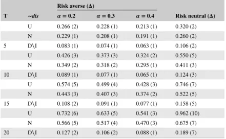
In this section we provide the numerical results related to the bilateral trade problem with risk-averse and risk-neutral interme-diary. Table 1 summarizes these results. The first column of the table entitled “T” specifies the cardinality of the sets where both seller and buyer valuations come from. The second column with “∼dis” label identifies the probability distribution of the
TABLE 1 Intermediary’s gains under risk-averse and risk-neutral approaches
Risk averse (𝚫)
T ∼dis 𝜶 = 0.2 𝜶 = 0.3 𝜶 = 0.4 Risk neutral (𝚫)
U 0.266 (2) 0.228 (1) 0.213 (1) 0.320 (2) N 0.229 (1) 0.208 (1) 0.191 (1) 0.260 (2) 5 D∖I 0.083 (1) 0.074 (1) 0.063 (1) 0.106 (2) U 0.426 (3) 0.373 (3) 0.324 (2) 0.550 (5) N 0.349 (2) 0.318 (2) 0.295 (1) 0.411 (3) 10 D∖I 0.089 (1) 0.077 (1) 0.065 (1) 0.124 (3) U 0.574 (5) 0.499 (4) 0.428 (3) 0.746 (7) N 0.443 (3) 0.407 (3) 0.374 (2) 0.522 (5) 15 D∖I 0.108 (2) 0.091 (1) 0.077 (1) 0.158 (5) U 0.732 (6) 0.633 (5) 0.541 (3) 0.962 (10) N 0.566 (5) 0.517 (4) 0.470 (3) 0.675 (7) 20 D∖I 0.127 (2) 0.106 (2) 0.088 (1) 0.189 (7)
seller and buyer valuations. We consider three specifications of distributions for this purpose. “U” stands for the uniform case where fi= T1 for all i and gj= T1 for all j. “N” mimics the normal distribution and is defined as follows; at first step we assign the value of|T| to the seller’s probability mass function with median index, say f̂i. Then, for the remaining elements assign the value using f̂i+
−k= |T| − 2.|k| formula and in the last step normalize them such that all elements sum up to one. The same
approach is applied for the buyer’s mass functions. Finally, “D∖I” refers to the case with increasing (decreasing) values of the seller’s (buyer’s) mass function probability. The applied rules are fi=|i| and gj=|T| − |j| + 1, then we also need to normal-ize the obtained values. The third column with three subcolumns provides the objective function value given by (11) and in fact is the gain of the risk-averse intermediary with three different confidence levels. The last column illustrates the expected gain of the risk-neutral intermediary. The value between parentheses, Δ, states the minimum difference between seller’s and buyer’s valuations where transaction may happen. For example, if the value is three, it means that in the optimal mechanism the transaction will not happen if the difference between the buyer’s and seller’s valuation is less than three.
We can observe from the table that when the level of risk-aversion increases the related objective function value decreases and the risk-neutral model gives higher objective value compared to the risk-averse one, which were the expectable results. We also observe that when level of risk-aversion increases the Δ value decreases. This means that when the intermediary becomes more risk-averse he prefers to allow the transaction to occur with smaller difference between the valuations of the seller and the buyer.
Another concluding remark which is not present in the table is that, in all instances presented in Table 1 the optimal value of the pijs are zero or one in the risk-neutral model but they take fractional value between zero and one in some cases of the
risk-averse model. As a result the optimal mechanism changes for the risk-averse intermediary who decides the allocation through a lottery in some realizations of the types.
5
C O N C L U D I N G R E M A R K S
In this paper, we dealt with bilateral trade with intermediary problem of microeconomic theory using tools of linear (network) programming duality. The problem is one of designing an optimal mechanism from the viewpoint of an intermediary bene-fiting from the difference between the buyer and seller valuations of the good to be exchanged. More precisely, a seller and a buyer, each withholding private information about an object, exchange it through an intermediary maximizing his/her expected gains from trade. In a Bayes-Nash equilibrium framework, we derived the optimal exchange mechanism using linear network optimization duality under discrete valuations of the two parties. Then we considered an extension where the intermediary also seeks to avoid risk. We also presented numerical results and discussed the main difference in the structure of optimal mechanism in both problems.
O R C I D
Halil ˙I. Bayrak https://orcid.org/0000-0002-7134-0833 Kamyar Kargar https://orcid.org/0000-0001-9405-5763 Mustafa Ç. Pınar https://orcid.org/0000-0002-8307-187X
R E F E R E N C E S
[1] R.K. Ahuja, T.L. Magnanti, and J.B. Orlin, Network Flows: Theory, Algorithms, and Applications, Prentice Hall, Inc., Upper Saddle River, NJ,
1993.
[2] P. Artzner, F. Delbaen, J.M. Eber, and D. Heath, Coherent measures of risk, Math. Finance 9 (1999), 203–228.
[3] J. Flesch, M. Schröder, and D. Vermeulen, Implementable and ex-post IR rules in bilateral trading with discrete values, Math. Social Sci. 84
(2016), 68–75.
[4] K. Kargar, H.I. Bayrak, and M.Ç. Pinar, Robust bilateral trade with discrete types, EURO J. Comput. Optimiz. 6 (2018), 367–393.
[5] P. Krokhmal, M. Zabarankin, and S. Uryasev, Modeling and optimization of risk, Surv. Oper. Res. Manag. Sci. 16 (2011), 49–66.
[6] R.B. Myerson, Optimal auction design, Math. Oper. Res. 6 (1981), 58–73.
[7] R.B. Myerson and M.A. Satterthwaite, Efficient mechanisms for bilateral trading, J. Econom. Theory 29 (1983), 265–281.
[8] A. Othman and T. Sandholm, “How pervasive is the Myerson-Satterthwaite impossibility?” Twenty-First International Joint Conference on
Artificial Intelligence, Morgan Kaufmann Publishers Inc., California, USA, 2009.
[9] M.Ç. Pinar, Robust trading mechanisms over 0/1 polytopes, J. Comb. Optim. 36 (2018), 845–860.
[10] R.T. Rockafellar and S. Uryasev, Optimization of conditional value-at-risk, J. Risk 2 (2000), 21–42.
[11] R.T. Rockafellar and S. Uryasev, Conditional value-at-risk for general loss distributions, J. Bank. Financ. 26 (2002), 1443–1471.
[12] D.F. Spulber, Market Microstructure: Intermediaries and the Theory of the Firm, Cambridge University Press, Cambridge, 1999.
[13] R.V. Vohra, Mechanism Design: A Linear Programming Approach, vol. 47, Cambridge University Press, Cambridge, 2011.
[14] R.V. Vohra, Optimization and mechanism design, Math. Programming 134 (2012), 283–303.
How to cite this article:Bayrak H˙I, Kargar K, Pınar MÇ. Bilateral trade with risk-averse intermediary using linear network optimization. Networks. 2019;74:325–332. https://doi.org/10.1002/net.21910