a thesis
submitted to the department of computer engineering
and the institute of engineering and science
of bilkent university
in partial fulfillment of the requirements
for the degree of
master of science
By
Atilla Genc.
January, 2010
Asst. Prof. Dr. ˙Ibrahim K¨orpeo˘glu(Supervisor)
I certify that I have read this thesis and that in my opinion it is fully adequate, in scope and in quality, as a thesis for the degree of Master of Science.
Dr. Cengiz C. elik(Co-Supervisor)
I certify that I have read this thesis and that in my opinion it is fully adequate, in scope and in quality, as a thesis for the degree of Master of Science.
Asst.Prof. Ali Aydın Sel¸cuk
Asst.Prof. ¨Ozcan ¨Ozt¨urk
I certify that I have read this thesis and that in my opinion it is fully adequate, in scope and in quality, as a thesis for the degree of Master of Science.
Asst.Prof. Tansel ¨Ozyer
Approved for the Institute of Engineering and Science:
Prof. Dr. Mehmet B. Baray Director of the Institute
QUERIES USING GRAPHIC PROCESSOR UNITS
Atilla Genc.
M.S. in Computer Engineering
Supervisor: Asst. Prof. Dr. ˙Ibrahim K¨orpeo˘glu Co-Supervisor: Dr. Cengiz C. elik
January, 2010
A Graphic Processing Unit (GPU) is primarily designed for real-time render-ing. In contrast to a Central Processing Unit (CPU) that have complex instruc-tions and a limited number of pipelines, a GPU has simpler instrucinstruc-tions and many execution pipelines to process vector data in a massively parallel fashion. In ad-dition to its regular tasks, GPU instruction set can be used for performing other types of general-purpose computations as well. Several frameworks like Brook+, ATI CAL, OpenCL, and Nvidia Cuda have been proposed to utilize computa-tional power of the GPU in general computing. This has provided interest and opportunities for accelerating different types of applications.
This thesis explores ways of taking advantage of the GPU in the field of metric space-based similarity searching. The KVP index structure has a simple organi-zation that lends itself to be easily processed in parallel, in contrast to tree-based structures that requires frequent ”pointer chasing” operations. Several imple-mentations using the general purpose GPU programming frameworks (Brook+, ATI CAL and OpenCL) based on the ATI platform are provided. Experimental results of these implementations show that the GPU versions presented in this work are several times faster than the CPU versions.
Keywords: Similarity Search, General Purpose Computing on Graphic Processing Units, GPGPU.
BENZERL˙IK SORGULARININ HIZLANDIRILMASI
Atilla Genc.
Bilgisayar M¨uhendisli˘gi, Y¨uksek Lisans Tez Y¨oneticisi: Asst. Prof. Dr. ˙Ibrahim K¨orpeo˘glu
Tez Y¨oneticisi: Dr. Cengiz C. elik Ocak, 2010
Grafik ˙I¸sleme Birimi (GPU) birincil olarak ger¸cek zamanlı g¨or¨unt¨u olu¸sturmak i¸cin tasarlanmı¸stır. Karma¸sık komut k¨umesi ve sınırlı ardı¸sık d¨uzene sahip merkezi i¸slem biriminin aksine GPU daha basit bir komut k¨umesine ve vekt¨or verilerini ko¸sut olarak ¸calı¸stırabilecek ¸cok sayıda y¨ur¨utme ardı¸sık d¨uzenine sahip-tir. Ola˘gan g¨orevlerine ek olarak, GPU komut k¨umesi ba¸ska tip genel ama¸clı hesaplamalar i¸cin kullanılabilir. GPU’ların i¸slem g¨uc¨un¨u genel ama¸clı hesapla-malarda de˘gerlendirebilmek i¸cin Brook+, ATI CAL, OpenCL ve Nvidia Cuda gibi de˘gi¸sik programlama ¸cer¸ceve modelleri ¨onerilmi¸stir. Bu durum pek ¸cok uygula-manın hızlandırılması i¸cin fırsat do˘gurmu¸stur.
Bu ¸calı¸smada metrik tabanlı benzerlik araması alanında grafik kartlarının sa˘gladı˘gı avantajların kullanılması incelenmektedir. Sık¸ca ”imle¸c takibi” gerek-tiren a˘ga¸c temelli yapıların aksine, KVP yapısı basit organizasyonu nedeniyle kolayca ko¸sut olarak i¸slenmeye uygundur. ATI platformunda de˘gi¸sik genel ama¸clı GPU programlama ¸cer¸ceve modelleri kullanılarak (Brook+, ATI CAL ve OpenCL) Brute Force Linear Scan ve KVP algoritmaları ger¸cekle¸stirilmi¸s, yapılan ¸calı¸sma sunulmu¸stur. Bu ger¸cekle¸stirimlerin deneysel sonuları GPU uygu-lamalarının CPU s¨ur¨umlerinden ¸cok daha hızlı oldu˘gunu g¨ostermektedir.
Anahtar s¨ozc¨ukler : Benzerlik Araması, Grafik ˙I¸sleme ¨Unitelerinde Genel Ama¸clı Hesaplama, GPGPU.
I would like to thank my supervisors, Asst. Prof. Dr. ˙Ibrahim K¨orpeo˘glu and Dr. Cengiz C. elik for their guidance throughout my study.
1 Introduction 1
2 Similarity Search 3
2.1 Overview . . . 3
2.2 Survey on Related Work . . . 9
2.2.1 Clustering-Based Methods . . . 11
2.2.2 Local Pivot-Based Methods . . . 12
2.2.3 Vantage-Point Methods . . . 14
2.3 KVP Algorithm . . . 16
2.3.1 The KVP Structure . . . 16
2.3.2 Secondary Storage . . . 18
2.3.3 Memory Usage . . . 19
2.3.4 Comparison of KVP and Tree-Based Structures . . . 20
3 General Purpose Computing On GPU 22 3.1 Overview Of Graphics Hardware . . . 24
3.1.1 Programmable hardware . . . 26
3.2 GPU Programming Model . . . 27
3.2.1 GPU Program Flow . . . 29
3.2.2 GPU Programming Systems . . . 32
3.2.3 GPGPU languages and libraries . . . 33
3.2.4 Debugging tools . . . 35 3.3 GPGPU Techniques . . . 37 3.3.1 Stream operations . . . 37 3.3.2 Data Structures . . . 43 3.4 GPGPU applications . . . 45 4 Implementation of Algorithms 52 4.1 Brute Force Search Implementation on GPU . . . 57
4.2 KVP Implementation GPU . . . 63
4.3 Filtering Results on GPU . . . 69
5 Experiment Results 75 5.1 Comparison of implementations with Result Set Filtering on CPU 77 5.2 Performance Overhead of Data Transfers from GPU to CPU . . . 81 5.3 Comparison of implementations with Result Set Filtering on GPU 86
2.1 Visualization of distance bounds. Given distances d(q, p) and d(p, o) upper and lower bounds on d(q, o) can be established us-ing triangle inequality (a) d(q, o) ≥ |d(q, p) − d(p, o)| (b) d(q, 0) ≤ d(q, p) + d(p, o) . . . 6 2.2 Possible partitioning of a set of objects. (a)ball partitioning and
(b) generalized hyperplane partitioning. . . 8 2.3 A sample database of 9 vectors in 2-dimensional space, and an
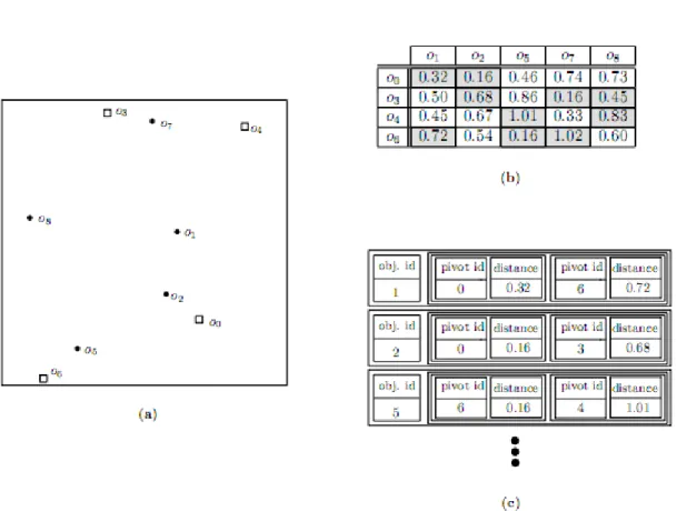
ex-ample of the KVP structure on this database that keeps 2 distance values per database object. (a) The location of objects. Boxes rep-resent objects that have been selected as pivots. (b) The distance matrix between pivots and regular database objects. For each ob-ject, the 2 most promising pivot distances are selected to be stored in KVP (indicated by using gray background color). (c) The first three object entries in the KVP. Each object entry keeps the id of the object, and an array of pivot distances. . . 18 2.4 Query performance of the KVP structure, for vectors uniformly
distributed in 20 dimensions. . . 19
3.1 The modern graphics hardware pipeline. The vertex and fragment processor stages are both programmable by the user. . . 25
4.1 Serialized representation of objects. . . 58 4.2 Packed instruction execution. . . 61 4.3 Iteratively counting number of objects in result set. . . 72
5.1 Execution times in seconds for 1000 radius queries on 220 vectors,
with varying vector dimensions. Result set filtering performed on CPU. . . 78 5.2 Relative speeds of implementations for test set 1, when result set
filtering is performed on CPU. . . 78 5.3 Execution times in seconds for 1000 radius queries on vectors with
16 dimensions and varying number of vectors. Result set filtering performed on CPU. . . 80 5.4 Relative speeds of implementations for test set 2, when result set
filtering is performed on CPU. . . 80 5.5 Execution times in seconds for 1000 radius queries on object set
size of 220 vectors, with varying vector dimensions, no result set fetching. . . 82 5.6 Relative speeds of implementations for test set 1, no result set
fetching. . . 82 5.7 Execution times in seconds for 1000 radius queries on vectors with
16 dimensions and varying number of vectors, no result set fetching.. 85 5.8 Relative speeds of implementations for test set 2, no result set
fetching. . . 85 5.9 Execution times for 1000 radius queries on object set size of 220
5.10 Relative speeds of implementations for test set 1, GPU result set filtering. . . 87 5.11 Execution times for 1000 radius queries on vectors with 16
dimen-sions and varying number of vectors, GPU result set filtering. . . 88 5.12 Relative speeds of implementations for test set 2, GPU result set
5.1 System configuration of Test Hardware . . . 76 5.2 Number of objects and dimension sizes used in measurements. . . 76 5.3 Execution times in seconds for 1000 radius queries on object set
size of 220 vectors, with varying vector dimensions. Result set
filtering performed on CPU. . . 77 5.4 Execution times in seconds for 1000 radius queries on vectors with
16 dimensions and varying number of vectors. Result set filtering performed on CPU. . . 79 5.5 Execution times in seconds for 1000 radius queries on object set
size of 220 vectors, with varying vector dimensions, no result set
fetching. . . 81 5.6 Data Transfer rate and percentage of time used in data transfers. 83 5.7 Execution times in seconds for 1000 radius queries on vectors with
16 dimensions and varying number of vectors, no result set fetching.. 84 5.8 Execution times in seconds for 1000 radius queries on object set
size of 220 vectors, with varying vector dimensions, GPU result set filtering. . . 86
5.9 Execution times in seconds for 1000 radius queries on vectors with 16 dimensions and varying number of vectors, GPU result set fil-tering. . . 86
Introduction
A very important issue on any kind of data management is searching. Traditional database systems efficiently search for structured records. However, the new data types like image, video, audio, protein structures etc. are not very structured and can not be handled efficiently. In these cases, the similarity search paradigm is a better solution. Similarity searching consists of retrieving data that are similar to a given query. The measure of similarity is specifically defined with respect to the target application.
One popular approach for similarity searching is mapping database objects into feature vectors, which introduces an undesirable element of indirection into the process. A more direct approach is to define a distance function directly between objects. Typically such a function is taken from a metric space, which satisfies a number of properties, such as the triangle inequality. Index structures that can work for metric spaces have been reported to outperform vector-based counterparts in many applications. Metric spaces also provide a more general framework, such as defining a distance between objects can be accomplished more intuitively than mapping objects to feature vectors for some domains.
Downside of using metric distance functions for similarity search is that they are usually computationally expensive. As computers find usage in new areas, new applications with complex similarity measures comes on demand, causing an
urgent need to improve the efficiency of similarity queries. Index structures that are designed for similarity search seek to reduce the number of distance compu-tations required to process a similarity search query. Another way of increasing speed of this expensive task is to find faster and more suitable configurations.
Recent graphics architectures provide tremendous memory bandwidth and computational horsepower. Their arithmetic power results from a highly special-ized architecture, evolved and tuned over years to extract maximum performance on the highly parallel tasks of traditional computer graphics. Also early GPUs were fixed-function pipelines whose output was limited to 8-bit-per-channel color values, whereas modern GPUs now include fully programmable processing units that support vectorized floating-point operations. The increasing flexibility of GPUs, coupled with some creative uses of that flexibility by GPGPU developers, has enabled many applications outside the original narrow tasks for which GPUs were originally designed. Researchers and developers have become interested in utilizing this power for general-purpose computing, an effort known collectively as GPGPU (for General-Purpose computing on the GPU). Thus these advances on graphic cards suggest it to be a viable and cheap opportunity for a faster computational hardware.
Objective of this thesis is to explore ways of taking advantage of the advances in GPU architectures in the field of similarity searching by accelerating execution times; specifically in brute force linear scan technique and KVP algorithm.
This thesis is organized as follows. Chapter 2 gives a broad survey on similarity searching and has a section specifically for discussions of KVP algorithm that will be implemented. Chapter 3 gives a broad survey on general purpose computation on graphical cards. In chapter, 4 implementation details of similarity search algorithms are presented. Chapter 5 reports experimental results obtained by measuring execution times of implementations in CPU and GPU environments through a set of tests. Finally, in chapter 5 concluding remarks are presented.
Similarity Search
2.1
Overview
One of the areas that computer systems had significant success is storage and retrieval of vast amounts of information. Many applications in computer science depend on efficient storage and retrieval of data. If data to be stored has some predefined structure, classical database methods that are designed to handle data objects provide quite a good performance. This predefined structure can be cap-tured by treating the various attributes associated with the objects as records and these records can be stored in the database using some appropriate model like relational, object-oriented, object-relational,hierarchical, network, etc. The retrieval process, responding to queries like exact match, range, and join applied to some or all of the attributes, is then facilitated by building indexes on the rel-evant attributes. As mentioned before these techniques assume some predefined structure and more importantly, concepts like data equality and similarity are well defined and evaluation of equality and similarity are not very costly.
As the proliferation of computer systems in data management increase, new demands on data storage and management arise. Recent applications require management of larger data as well as storage and retrieval of data which has considerably less structure. A few examples of such data and applications of the
similarity search include: audio and image databases [21], video,audio recordings, text documents, time series, DNA sequences, fingerprints [59], face recognition [58] etc. Such data objects sometimes can be described via a set of features, which is called a feature vector. Feature vectors consists of features which are scalar values. For example, in the case of image data, the feature vector might include color, color moments, textures, or RGB values of the image pixels etc. which are scalar values. In the case of text documents, we might have one dimension per word, which can lead to prohibitively high dimensions. Also there are some cases where, even a feature vector may not be available. Sometimes we only have a set of objects and a distance function d, which is usually quite expensive to compute, where d specifies the degree of similarity (or dissimilarity) between all pairs of objects. The challenge with these kind of data is that usually the data can not be ordered and most of the time it is not meaningful to perform equality comparisons on it. To illustrate the point, consider retrieval of songs that are similar to a query song from a set of songs, or finding a images which contain a certain person from a set of images. When dealing with cases where data can not be sorted, nor a clear definition of equality or similarity can be provided, proximity becomes more appropriate retrieval criterion and queries can be defined as:
1. Finding objects whose feature values fall within a given range or where the distance, using a suitably defined distance metric, from some query object falls into a certain range (range queries).
2. Finding objects whose features have values similar to those of a given query object or set of query objects (nearest neighbor queries). In order to reduce the complexity of the search process, the precision of the required similarity can be an approximation (approximate nearest neighbor queries).
3. Finding pairs of objects from the same set or different sets which are suffi-ciently similar to each other (closest pairs queries).
The process of computing results to these queries is termed similarity search-ing.
The main problem with processing similarity search queries is the difficulty with dealing very large dimensions and cost of evaluating distance functions which are usually expensive to compute. Thus a good indexing method should be able to deal with high dimensions of data and/or reduce the number of distance computations to evaluate query.
If data can be modeled by feature vectors one can form indexes on various features as in the case of structured data and use point access methods (eg., [24, 77, 78]). These feature vectors are represented as coordinate vectors. In these approaches, it is assumed that the objects can be decomposed into or represented as vectors over some multi-dimensional space, and distances are measured using geometric distance functions like standard Euclidean distance. Numerous index structures have been created based on this approach. One of the drawbacks of this approach is that it is not being suitable for wide range of applications, as it may not be possible to represent data as feature vectors.
An alternative direction for research had been similarity search in the more general setting of metric spaces. In this thesis we focus on similarity search methods which assume similarity is defined using a metric distance function. A metric space is defined to be a set of objects S together with a distance function d on pairs of objects that satisfies the following properties ∀a, b, c ∈ S
1. Positivity: d(a, b) ≥ 0, d(a, a) = 0 2. Symmetry: d(a, b) = d(b, a).
3. Triangle Inequality: d(a, b) + d(b, c) ≥ d(a, c).
Positivity property ensure that distance function is defined for pair of objects and distance is not negative. Also it ensures that distance of some object to itself is zero, minimum possible distance, corresponding to intuitive notion object is similar to itself. Symmetry property ensures distance between two object are same regardless of the direction.
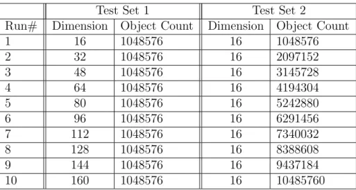
Of the distance metric properties, the triangle inequality is the key property for pruning the search space when processing queries. However, in order to make
use of the triangle inequality, we often find ourselves applying the symmetry property. Furthermore, the non-negativity property allows discarding negative values in formulas. The triangle inequality dictates that the distance between two objects is closely related to their distances to a third object. This relation can be seen Figure 2.1. Given distances d(q, p) and d(p, o) upper and lower bounds on d(q, o) can be established.
Figure 2.1: Visualization of distance bounds. Given distances d(q, p) and d(p, o) upper and lower bounds on d(q, o) can be established using triangle inequality (a) d(q, o) ≥ |d(q, p) − d(p, o)| (b) d(q, 0) ≤ d(q, p) + d(p, o)
Metric-space indexing structures exploit this fact by appointing a small set of objects to represent the whole population. These objects are called pivots or vantage points. The distances between the pivots and a set of database objects are precomputed and stored in the index structure. At query time, the distance between some of the pivots and the query object is computed. Using the triangle inequality, the distance between a regular database object and the query object can be bounded by their distances to the pivots. If the lower bound of the distance between a database object and the query object is greater than the query radius, it follows that the object is outside the query range, and the object can be eliminated from consideration. In a similar fashion, if the upper bound of the distance is less than the query radius, it follows that the object lies within the range. We call this operation pivoting. Objects that have been classified in this manner are said to be eliminated. Database objects that are not eliminated must have their distances to the query object computed explicitly. The efficiency of an index structure is directly related to the fraction of database objects that can be eliminated through pivoting.
internal structure about objects as long as distance function is defined over all pair of objects in the collection. This level of abstraction enables us the capability of capturing a large variety of similarity search applications. It provides a natural and intuitive way to approach a problem. For example, the distance between two character strings may easily be determined by the edit distance, which is a metric [53]. On the other side, this level of abstraction eliminates some constraints which could be useful in building indexes. For example, vector-based methods can enhance efficiency by processing the dimensions of the vector one at a time. An example of this is incremental distance computation [3], where the distance of the query object to a bounding box is computed one dimension at a time. Another example is the TV-tree [55]. In the TV-tree, new dimensions are introduced only as they are needed.
The advantage of distance-based indexing methods is that once the index has been built, similarity queries can often be performed with a significantly lower number of distance computations than a sequential scan of the entire dataset, as would be the case if no index exists. Another advantage over the multidimen-sional indexing methods is that different distance metrics can be defined objects and used to index them. Of course, in situations where we may want to apply several different distance metrics, then distance-based indexing techniques have the drawback of requiring that the index be rebuilt for each different distance metric.
There are two main approaches when only distance functions are used in similarity search. First method is to derive artificial features based on inter object distances (e.g., methods described in [22, 42, 57, 89]). In these approaches, goal is to find a mapping F that is defined for all elements of S and query objects which maps original objects to points in k-dimensional space. New distance function de defined in k-dimensional space should be as close as possible original distance
function d. The advantage of this approach is that it replaces original function d with a new function de which is expected to be much less expensive. Another
advantage of this approach is that after mapping new points can be indexed using multidimensional indexes. These methods are known as embedding methods and they are also applicable if objects are represented as feature vectors. Advantage
of using embedding methods on features vectors is reduction in the number of dimensions, if the dimensions of newly mapped space k, is smaller than original dimensions of feature vector.
An important constraint on embedding methods is that the mapping F should be contractive [39], which implies that it does not increase the distances between objects. That is, de(F (o1), F (o2)) ≤ d(o1, o2)∀o1, o2 ∈ S. This property ensures
that there will be no incorrect elimination of objects when processing query using new mapped space and new distance function. Results are later refined using d (e.g., [48, 79]).
Another approach which is used when only distance functions are known is to index objects with respect to their distances from a few selected objects called pivots. Almost all existing index structures for metric similarity search are built around the concept of pivoting. They differ in the way they select pivots, which objects are associated with each pivot, how the pivot distances will be organized and how pivots separate objects. These differences also affect how the querying process will be carried out.
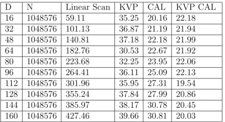
Deciding how pivots partition data is also a differentiating factor among sim-ilarity search algorithms. [85] identified two basic partitioning schemes, ball par-titioning and generalized hyperplane parpar-titioning.
Figure 2.2: Possible partitioning of a set of objects. (a)ball partitioning and (b) generalized hyperplane partitioning.
distinguished object, sometimes called a vantage point [93], that is, into the subset that is inside and the subset that is outside a ball around the object (e.g., Figure 2.2(a)).
In generalized hyperplane partitioning, two distinguished objects a and b are chosen and the data set is partitioned based on which of the two distinguished objects is the closest, that is, all the objects in subset A are closer to a than to b, while the objects in subset B are closer to b (e.g., Figure 2.2(b)).
2.2
Survey on Related Work
Some of the earliest distance-based indexing methods are due to [14], but most of the work in this area has taken place in the past decades. Typical of distance based indexing structures are metric trees [85], which are binary trees that result in recursively partitioning a data set into two subsets at each node. The VP-tree [93] stands out as one requiring only a small amount of memory and being able to be constructed efficiently. However it is inferior to others in terms of query performance, including methods like the MVP-tree [9], and GNAT [10], both of which improve performance at the cost of greater space and construction time.
The M-tree [17] and Slim-tree [44] are disk-based structures, and support dynamic manipulations on the index while maintaining the balance of the tree. In order to be able to efficiently handle split and merge operations, however, they keep less precise data than the comparable GNAT structure. This results in poorer query performance.
While most distance based indexing structures are variations on and/or exten-sions of metric trees, there are also other approaches. Several methods based on distance matrices have been designed [65, 87, 88]. In these methods, all or some of the distances between the objects in the data set are precomputed. Then, when evaluating queries, once we have computed the actual distances of some of the objects from the query object, the distances of the other objects can be estimated based on the precomputed distances. Clearly, these distance matrix methods do
not form a hierarchical partitioning of the data set, but combinations of such methods and metric tree-like structures have been proposed [64]. The SA-tree [66] is another departure from metric trees, inspired by the Voronoi diagram. In essence, the SA-tree records a portion of the Delaunay graph of the data set, a graph whose vertices are the Voronoi cells, with edges between adjacent cells.
Tree structures typically only allow an object to have as many pivots as the height of the tree. This may not be satisfactory for difficult distributions and queries. For this reason tree-based structures are not flexible enough to provide greater elimination power when needed. In contrast, vantage point structures like LAESA [65], Spaghettis [15] and FQA [16] represent another family of solu-tions. They use more space and construction time, but provide greater efficiency at query time. Although other tree structures also have some parameters that can be adjusted, their improvements are not as pervasive or as dramatic. The shortcomings of vantage points-based methods are the extra computational over-head that they incur, higher construction costs, and higher space usage. If they are allowed to use a sufficient number of pivots, these methods have been shown to outperform other methods in terms of the number of distance computations performed. Some of the structures in this family offer some improvements to the common problems of high space and construction time. The Spaghettis structure reduces computational overhead but uses more space than the common approach. The FQA also reduces overhead, but it uses less precision in the distance informa-tion it stores, resulting in reduced performance in terms of the number of distance computations.
Further material on similarity search methods can be found at [66] and [38] which are very good surveys on similarity search.
In the following sections we report similarity search methods under three broad categories: Clustering-based methods, local pivot-based methods, and vantage points-based methods.
2.2.1
Clustering-Based Methods
The basic theme behind clustering-based methods is the use of a hierarchical, tree-based decomposition of the space, where the subtrees are designed to group close objects together. We also observe that each subtree is represented by a single object from the database that is ideally located near the center of the group of objects stored in this subtree.
J. Uhlmann [85] defined the gh-tree, short for generalized hyperplane tree, as one of the first examples in this category. The idea is to pick two objects from the current subset as representatives, and partition the rest of the set into two classes, depending on which representative is closer.
The GNAT tree, presented by S. Brin [10] is a generalization of the gh-tree, where there are more than two representatives. A simple algorithm is given to pick the representatives. According to the algorithm, if we are to select k repre-sentatives, we first pick 3 · k points randomly. Then, starting with an initial set consisting of one random representative, we incrementally grow the set by adding the point that maximizes the minimum distance to the other representatives.
In addition to its representatives, each node can also maintain the radius of the associated region, that is, the maximum distance of the objects inside a represen-tatives region. This method was used in the M-tree (described below). Another enhancement would be to include the distances between the representatives as well. An even more precise way is used in the GNAT tree. Every representative stores the minimum and maximum distances to the objects in every other subset. The performance of GNAT, in the best case, has been reported to make more than a factor of 6 fewer distance computations than the VP-tree, while requiring about a factor of 14 more in distance computations in its construction. How-ever, it was reported to be worse than the VP-tree in some cases. The original study [10] also showed that GNAT was outperformed by a variant of the vantage points structure, although no data was given about the parameters used in the construction of this structure. Recent experiments presented by [66], [16] show
indeed that GNAT performs consistently worse than variants of vantage points structures in terms of number of distance computations, while it consumes less space and has less computational overhead.
The M-tree [17] is designed to be a dynamic structure, with emphasis being paid to the structures ability to perform queries efficiently and to optimize I/O performance after a sequence of data insertions. Similar to SS-tree [90], it keeps the distance to the farthest object in a subtree. Maintaining the radius of the representative objects allows it to easily reorganize disk blocks. Splitting a node involves selecting two new representatives and redistributing objects associated with this node among these two new nodes. The M-tree considers all possibilities for a split and chooses the one with tightest covering radius.
The Slim-tree [44] employs a more efficient splitting method. The minimum spanning tree of the objects is generated and the longest arcs of the spanning tree is removed partition the set of objects into two subsets.
2.2.2
Local Pivot-Based Methods
The structures in this category are also tree-based, however, the partitions are based on the distances of objects to either one or two selected objects called pivots. Objects that have similar distances to the pivots are put inside the same subtree, but that does not necessarily mean they are in close proximity of each other. The pivots are only used within their subset, and this is why we call them local pivots. W. Burkhard and R. Keller [14] suggested selecting a random object in the data set and partitioning the rest such that every object having the same distance to the preselected object is placed in the same subset. The tree construction continues recursively on the subset of points at the same distance. Since their application domain produced discrete distance values, it was possible for many points to be at the same distance.
An adaptation of the same basic idea to continuous distance values is the VP-tree, [93]. Such a tree is defined by a branching factor. In order to construct
a vp-tree with a given branching factor k, at a given node, one of the objects is selected as the vantage point, and the distances from the other objects to this vantage point are calculated. Then these objects are partitioned into k groups of roughly equal size based on these distances. In this way a node can have k branches with each subtree having roughly m/k objects, where m denotes the number of objects for that node. The only information that needs to be stored is the vantage point itself, and the k − 1 distance values, denoted as cutoff[1..k], defining the ranges of distances for each subtree.
A range query of radius r centered at a query point q is answered as follows: at any given node, the distance d between q and the nodes vantage point is calculated. If d is smaller than r, the vantage point is added into the result set. For every subset i of the node defined by the cutoff values, if the interval of the subset, [cutoff [ i − 1 ], cutoff [i]] intersects the interval [d − r, d + r], then subset i is searched recursively.
A nice feature of the VP-tree is that it is possible to divide the space into many divisions through a single distance calculation. As a result, when doing a search, we need only perform one distance calculation per node. However, as the dimensionality of the data distribution grows, it is well known that for many distributions, the objects tend to cluster around a single distance value [5]. As a result, almost all of the objects are at the same distance to the vantage point. Thus, the distance to the vantage point loses its discriminating power with respect to the objects. Another common way to describe the situation is to visualize the situation in a 3 dimensional space, where the median spheres dividing the branches have very similar radii, subdividing space into thin spherical shells. As a result, objects that are grouped under same subtree tend to be spread around the space rather being close to one another.
The MVP-tree [9] uses two vantage points per node. After partitioning the points with one primary vantage point, the partitions are further divided by using the second vantage point. This way, if we divide the space into m different regions by first vantage point, we will have a total of up to m2 subsets. It should be noted that the second vantage point uses different cutoff values for each partition
of the first vantage point. This allows the tree to maintain balance by assigning approximately the same number of points to each subset. This occurs at the cost of more space consumption per node. The value of this partitioning approach is that, instead of dividing the space into very thin shells, it strives to produce more tightly clustered subsets, while still achieving the same fanout.
The MVP-tree stores distances to two vantage points at the leaf nodes, making it a hybrid of the vantage-point structures. It is reported to perform up to 80
2.2.3
Vantage-Point Methods
In vantage-point methods the pivots are used to control processing for the entire set of objects instead of having local scope as they do in the previously described methods. A subset of the objects are selected as vantage points. The distance between the pivots and the rest of the objects are computed at initialization time and stored in the database. At query time these precomputed distances are used to eliminate candidates in a way that is similar to local methods. If there are k vantage points, then the basic method performs k · n distance computations at construction and keeps k · n distance values in the index structure. A range query accesses these distance values to determine which objects can be eliminated based on their distances to vantage points. Finally, a pass through all objects not eliminated by use of pivots is performed.
Note that vantage-point methods require extra processing compared to local methods, where determination of the partition at a node is done only for the objects covered by the node. Local methods require storage that is only linear in the database size, whereas vantage-point methods require O(k · n) storage.
A powerful aspect of these methods is that it is possible to use as many pivots as desired at the cost of construction time, which results in higher storage requirements and extra preprocessing time. Nonetheless, this additional effort and space can yield progressively better query performance in terms of the number of distance computations.
The first vantage-point structure that appeared in literature was LAESA [65], as a special case of AESA [87]. There have been some improvements over the basic LAESA algorithm, such as keeping distances to the vantage points sorted and doing binary searches to identify which objects can be eliminated from con-sideration [67].
The TLAESA structure [64] was proposed as a hybrid method between the LAESA and the gh-tree. The pivots are organized as in a gh-tree, but a distance matrix is also used to provide lower bounds for the distance of the query object to the node representatives. Their experiments were performed in low dimensions, and although were superior to LAESA in terms of total CPU cost, it was inferior in terms of the number of distance computations.
The Spaghettis structure [15] was introduced as a method designed to further decrease computational overhead. Here the distances are sorted in a similar fashion. In addition, every distance has a pointer for the same objects distance in the next array of distances. As done in the case of sorted distances, the feasible ranges are computed for each array using binary search. For each point, its path starting from first array is traced using the pointers. Once the object falls out of range in any of the arrays, we may infer that the object cannot lie within the query region.
The Fixed Queries Array (FQA) [16] is one of the recent global pivot-based methods. It sorts the points according to their distances to the first vantage point, then on the second, and so on. It decreases the precision with which distances are measured, for otherwise the points effectively would be sorted only in their distance to the first pivot. Using this sorted structure, the query algorithm performs binary searches within each distance range. The first pivot is processed as in the sorted-array approach, after that, for each range of objects that has the same discretized distance to the first vantage point, we perform a binary search to find the range that is valid for the second pivot. The search continues in this fashion performing binary searches within ranges.
FQA is unique among vantage-point methods that are designed to reduce com-putational overhead in that it does not require any additional storage. However
it does not work very well if too many bits are used for the distance values, since this would require that the structure be sorted only by the first pivot. This cre-ates an additional trade-off between the number of bits used for distance storage and extra CPU processing time needed. This comes in addition to the trade-o between number of bits and query performance in terms of distance computa-tions. Their experiments show great improvements in low dimensions, but for 20 dimensional data for a database of one million objects, they estimate FQA would take only 37.6
2.3
KVP Algorithm
In this section KVP structure [18], will be introduced in detail. This structure is unique since it improves both the storage and computational overhead of the classical vantage-points approach. The KVP structure offers a number of benefits:
1. It is a simple data structure and can be implemented relatively easily. 2. It can support dynamic operations like insertion and deletion.
3. It is easily adapted for use as a disk-based structure and its access patterns minimize the number of disk-seek operations.
4. Queries may be executed in parallel.
2.3.1
The KVP Structure
In vantage points all pivots are kept in structure even though not all of them may be useful in query evaluation. In [18], it is reported that it is desirable to use pivots that are particularly close to the query object. Similarly, a pivot to be more effective for objects that are close to or distant from it. This suggest an improvement over keeping all pivots, at index creation time, one can find pivots that are more close or distant to a object, and choose to keep only the distances to these promising pivots.
This is indeed what is done with KVP, the distance relations between the pivots and database elements are computed beforehand at construction time. In addition to reducing CPU overhead by first processing the most promising pivots, one can eliminate distance computations to the less promising pivots, thus decreasing the space requirements. There are two ways this can be implemented. One way would involve the usual layout, where every pivot stores an array of distances to all the database objects. The object distances can be sorted so that binary search can be used to quickly determine set of objects that are eliminated. Another way to implement the basic idea is to have a collection of object entries, where each object entry stores the distances to its selected pivots. The benefit of this latter approach is that it is very easy to insert or delete objects from the database, since there is no global data structure that keeps information about the objects. KVP takes the second approach. Figure 2.3 illustrates the approach.
Other than the fact that KVP only stores a subset of pivot distances, the way it processes queries is identical to the classical global pivot-based method. For each database object it maintains a lower and upper bound for the distance to the query object. Each pivot is used to attempt to tighten these bounds. After processing all possible pivot distances, if the bounds are good enough to either discard the object as out of the query range, or prove that it is within the query range, one avoids computing the actual distance between the object and the query object. Otherwise this distance is computed.
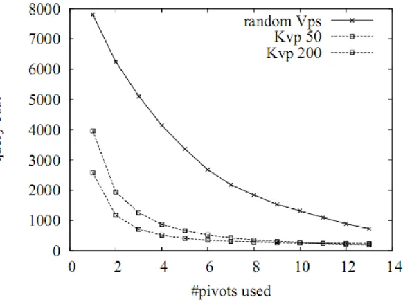
Figure 2.4 shows the query performance of KVP as a function of the number of pivots stored for a query radius of 0.4 in 20 dimensions. The results that are labeled as random choose the next pivot to be used randomly, simulating a classic vantage-points structure. KVP methods first process close and distant vantage points. For example, assume we have a KVP structure that has a pool of 50 prioritized vantage points, which we refer to as KVP 50. In the sorted array of pivot distances 0 through 49, the processing proceeds in the order: 0, 49, 1, 48, 2, and so on. As the number of pivots in the pool is increased, the chances of finding a better suited pivot also increases. Varying the number of pivots provides flexibility to improve query performance by spending more time at construction time without increasing space and CPU overhead.
Figure 2.3: A sample database of 9 vectors in 2-dimensional space, and an ex-ample of the KVP structure on this database that keeps 2 distance values per database object. (a) The location of objects. Boxes represent objects that have been selected as pivots. (b) The distance matrix between pivots and regular database objects. For each object, the 2 most promising pivot distances are se-lected to be stored in KVP (indicated by using gray background color). (c) The first three object entries in the KVP. Each object entry keeps the id of the object, and an array of pivot distances.
As seen from the graphs that KVP, can eliminate database objects much faster than the classic approach.
2.3.2
Secondary Storage
Access patterns of pivot-based structures are targeted toward minimizing CPU time, but they are not always suitable to be stored on disk. For example, per-forming binary search in secondary storage is expensive as it involves many seek
Figure 2.4: Query performance of the KVP structure, for vectors uniformly dis-tributed in 20 dimensions.
operations. Disks are much better at performing sequential scans. The KVP structure is quite amenable for data that are stored on disk. It only requires a sequential scan of distance values. It does not involve a heavy processing burden, so processing time does not dominate over I/O time. It requires relatively little memory, since only the vantage objects, the query object, and the distance vector of the processed object is needed.
2.3.3
Memory Usage
KVP and its variants HKvp and EcKvp store fewer distance values than the clas-sic vantage-point methods [18]. Depending on the parameters of KVP structure, memory usage of KVP changes. KVP structure keeps tracks of indexes used in structure. Also for each object a subset of pivots is selected, and distance from
object to selected pivots is precomputed and stored.
For object collection of n objects, if bd bits are used for distance values and
bi bits are used for indexes of pivots, and assuming npivot selected in index
con-struction with npivotlimit limit per object, memory usage of KVP is mKV P,
mKV P = n × (npivotlimit× (bd+ bi)) + npivot∗ bi
As with FQA, KVP can decrease memory consumption by discretization, so that fewer bits are used for the distance values. Consider its simplest form where the intervals have equal width, using b bits in a metric space where the maximum distance is Dmax. This will map distances into buckets of width Dw where
Dw = Dmax2b
Since all the distances in the same bucket will be assigned the same distance value, the maximum error will be Dw per distance value. Assuming query objects
are distributed uniformly, we can approximate the error toDw/2 .
Therefore, query process is modified to use r +Dmax
2 , instead of r and rest of
al-gorithm stays same. This discretization can improve memory usage considerably, since can be very large n.
2.3.4
Comparison of KVP and Tree-Based Structures
Using a KVP structure, one can easily vary a number of parameters, including the construction cost, the number of pivots used per object, the number of pivots stored per object, the number of pivots processed at query time per object, and the number of bits used per distance value.
In a sense, it is possible to view most of the existing structures as variants of the vantage point-based methods. For example in a VP-tree with a branching fac-tor of k, there is one pivot per node, all the objects in subtrees can be eliminated with their distances to this pivot, and number of branches have an affect similar to the number of bits used. For a database object, there are approximately as
many pivots as the height of the tree. This view explains why changing k in the VP-tree has little affect on query performance, since as k increases and pivots become more precise (which is similar to using more bits), the height of the tree becomes shorter and there are fewer pivots per database object. A major problem with the VP-tree is that the only data that is used are the cutoff values. The individual distances of objects to the pivots are computed but then discarded.
From the perspective of vantage points, it is also easier to see why GNAT with branching factor k improves on the VP-tree. In GNAT, there are k pivots per node, and the distance ranges of k subtree to these pivots are stored. One slight disadvantage of GNAT is that ranges of distances to a pivot can overlap. However, instead of having just one pivot per one, objects in GNAT make use of k pivots.
Tree-based methods have two advantages over the classical vantage points methods. Whereas a pivoting operation involves one object in vantage points, it usually involves groups of objects in tree-based structures. This is something that only cause increase on the CPU overhead, and has a negative impact on the number of distance computations. Secondly, tree-based methods attempt to divide the space into clusters in order to benefit from the locality of pivots. This is similar to what priority vantage points and KVP try to accomplish. While tree structures have varying degrees of success in clustering similar objects to-gether, KVP takes a direct approach and precisely computes the closest pivots. In addition, KVP properly makes use of far pivots as well.
General Purpose Computing On
GPU
Recent developments on graphics chips, known generically as Graphics Processing Units or GPUs, have provided a quite powerful computational units. Researchers and developers have become interested in utilizing this power for general purpose computing, an effort known collectively as GPGPU (for General Purpose com-puting on the GPU). In this section we summarize the efforts in field of GPGPU, give an overview of the techniques and computational building blocks used to map general purpose computation to graphics hardware, and survey the various general purpose computing tasks to which GPUs have been applied. A quite good survey on this field is provided by Owens et al. [71], which this section is based. Recent graphics architectures provide tremendous memory bandwidth and computational horsepower. For example, the flagship ATI Radeon HD 5970 ($625 as of January 2010) boasts 256.0 GB/sec memory bandwidth; with 4.64 TeraFLOPS theoretical single precision processing power. Similarly competitor NVIDIA’s flagship product GeForce 295 GTX ($475 as of January 2010) has 223.8 GB/sec memory bandwidth. GPUs also use advanced processor technol-ogy; for example, the ATI HD 5970 contains 4.3 billion transistors and is built on a 40-nanometer fabrication process.
Graphics hardware is fast and getting faster quickly. In fact graphics hard-ware performance increasing more rapidly than that of CPUs. The disparity can be attributed to fundamental architectural differences: CPUs are optimized for high performance on sequential code, with many transistors dedicated to extract-ing instruction-level parallelism with techniques such as branch prediction and out-of-order execution. On the other hand, the highly data-parallel nature of graphics computations enables GPUs to use additional transistors more directly for computation, achieving higher arithmetic intensity with the same transistor count.
Modern graphics architectures have become flexible as well as powerful. Early GPUs were fixed-function pipelines whose output was limited to 8-bit-per-channel color values, whereas modern GPUs now include fully programmable processing units that support vectorized floating point operations on values stored at full IEEE single precision (but note that the arithmetic operations themselves are not yet perfectly IEEE-compliant). High level languages have emerged to support the new programmability of the vertex and pixel pipelines [12, 61, 62]. Additional levels of programmability are emerging with every major generation of GPU (roughly every 18 months). For example, current generation GPUs introduced vertex texture access, full branching support in the vertex pipeline, and limited branching capability in the fragment pipeline. The next generation will expand on these changes and add geometry shaders, or programmable primitive assembly, bringing flexibility to an entirely new stage in the pipeline [6]. The raw speed, increasing precision, and rapidly expanding programmability of GPUs make them an attractive platform for general purpose computation.
Yet the GPU is hardly a computational panacea. Its arithmetic power results from a highly specialized architecture, evolved and tuned over years to extract maximum performance on the highly parallel tasks of traditional computer graph-ics. The increasing flexibility of GPUs, coupled with some ingenious uses of that flexibility by GPGPU developers, has enabled many applications outside the orig-inal narrow tasks for which GPUs were origorig-inally designed, but many applications still exist for which GPUs are not (and likely never will be) well suited. Word processing, for example, is a classic example of a pointer chasing application,
dominated by memory communication and difficult to parallelize.
Todays GPUs also lack some fundamental computing constructs, such as effi-cient scatter memory operations (i.e., indexed write array operations) and integer data operands. The lack of integers and associated operations such as bit-shifts and bitwise logical operations (AND, OR, XOR, NOT) makes GPUs ill-suited for many computationally intense tasks such as cryptography (though upcoming Direct3D 10 class hardware will add integer support and more generalized in-structions [6]). Finally, while the recent increase in precision to 32-bit floating point has enabled a host of GPGPU applications, 64-bit double precision arith-metic remains a promise on the horizon. The lack of double precision hampers or prevents GPUs from being applicable to many very large scale computational science problems.
Furthermore, graphics hardware remains difficult to apply to non-graphics tasks. The GPU uses an unusual programming model, so effective GPGPU pro-gramming is not simply a matter of learning a new language. Instead, the com-putation must be recast into graphics terms by a programmer familiar with the design, limitations, and evolution of the underlying hardware. Today, harnessing the power of a GPU for scientific or general purpose computation often requires a concerted effort by experts in both computer graphics and in the particular computational domain. But despite the programming challenges, the potential benefits, a leap forward in computing capability and a growth curve much faster than traditional CPUs are too large to ignore.
3.1
Overview Of Graphics Hardware
In this section we will outline the evolution of the GPU and describe its current hardware and software.
3D graphics applications require high computation rates and exhibit substan-tial parallelism which differentiate it from more general computation domains. Graphic cards are designed to take advantage of the native parallelism in the
application, allowing higher performance on graphics applications than can be obtained on more traditional microprocessors.
All of today’s commodity GPUs structure their graphics computation in a similar organization called the graphics pipeline. This pipeline is designed to allow hardware implementations to maintain high computation rates through parallel execution. The pipeline is divided into several stages. All geometric primitives pass through each stage: vertex operations, primitive assembly, rasterization, fragment operations, and composition into a final image. In hardware, each stage is implemented as a separate piece of hardware on the GPU in what is termed a task parallel machine organization. Figure 3.1 shows the pipeline stages in current GPUs. For more detail on GPU hardware and the graphics pipeline, NVIDIA’s GeForce 6 series of GPUs is described by Kilgariff and Fernando [47]. From a software perspective, the OpenGL Programming Guide provides an excellent reference [69].
Figure 3.1: The modern graphics hardware pipeline. The vertex and fragment processor stages are both programmable by the user.
3.1.1
Programmable hardware
The graphics pipeline described above was historically a fixed function pipeline, where the limited number of operations available at each stage of the graphics pipeline were hardwired for specific tasks. However, the success of off-line ren-dering systems such as Pixars RenderMan [86] demonstrated the benefit of more flexible operations, particularly in the areas of lighting and shading. Instead of limiting lighting and shading operations to a few fixed functions, RenderMan evaluated a user defined shader program on each primitive, with impressive visual results.
Over the past seven years, graphics vendors have transformed the fixed func-tion pipeline into a more flexible programmable pipeline. This effort has been primarily concentrated on two stages of the graphics pipeline: the vertex stage and the fragment stage. In the fixed function pipeline, the vertex stage included operations on vertices such as transformations and lighting calculations. In the programmable pipeline, these fixed function operations are replaced with a user defined vertex program. Similarly, the fixed function operations on fragments that determine the fragment’s color are replaced with a user defined fragment program.
Each new generation of GPUs has increased the functionality and generality of these two programmable stages. 1999 marked the introduction of the first pro-grammable stage, NVIDIA’s register combiner operations that allowed a limited combination of texture and interpolated color values to compute a fragment color. In 2002, ATI’s Radeon 9700 led the transition to floating point computation in the fragment pipeline.
The vital step for enabling general purpose computation on GPUs was the introduction of fully programmable hardware and an assembly language for spec-ifying programs to run on each vertex [56] or fragment. This programmable shader hardware is explicitly designed to process multiple data parallel primitives at the same time. In general, these programmable stages input a limited number of 32-bit floating point 4-vectors. The vertex stage outputs a limited number of
32-bit floating point 4-vectors that will be interpolated by the rasterizer; the fragment stage outputs up to 4 floating point 4-vectors, typically colors. Each programmable stage can access constant registers across all primitives and also read-write registers per primitive. The programmable stages have limits on their numbers of inputs, outputs, constants, registers, and instructions; with each new revision of the vertex shader and pixel [fragment] shader standard, these limits have increased.
GPUs typically have multiple vertex and fragment processors. Fragment pro-cessors have the ability to fetch data from textures, so they are capable of memory gather. However, the output address of a fragment is always determined before the fragment is processed, and the processor cannot change the output location of a pixel. Vertex processors recently acquired texture capabilities, and they are capable of changing the position of input vertices, which ultimately affects where in the image pixels will be drawn. Thus, vertex processors are capable of both gather and scatter. Unfortunately, vertex scatter can lead to memory and ras-terization coherence issues further down the pipeline. Combined with the lower performance of vertex processors, this limits the utility of vertex scatter in current GPUs.
3.2
GPU Programming Model
GPUs are a compelling solution for applications that require high arithmetic rates and data bandwidths. GPUs achieve this high performance through data paral-lelism, which requires a programming model distinct from the traditional CPU sequential programming model. In this section, we briefly introduce the GPU programming model using both graphics API terminology and the terminology of the more abstract stream programming model, because both are common in the literature.
patterns inherent in the application by structuring data into streams and ex-pressing computation as arithmetic kernels that operate on streams. Owens [70] discuss the stream programming model in the context of graphics hardware, and the Brook programming system [12] offers a stream programming system for GPUs.
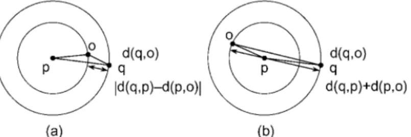
Because typical scenes have more fragments than vertices, in modern GPUs the programmable stage with the highest arithmetic rates is the fragment stage. A typical GPGPU program uses the fragment processor as the computation engine in the GPU. Such a program is structured as follows [32]:
1. First, the programmer determines the data parallel portions of his applica-tion. The application must be segmented into independent parallel sections. Each of these sections can be considered a kernel and is implemented as a fragment program. The input and output of each kernel program is one or more data arrays, which are stored (sometimes only transiently) in textures in GPU memory. In stream processing terms, the data in the textures com-prise streams, and a kernel is invoked in parallel on each stream element. 2. To invoke a kernel, the range of the computation (or the size of the output
stream) must be specified. The programmer does this by passing vertices to the GPU. A typical GPGPU invocation is a quadrilateral (quad) oriented parallel to the image plane, sized to cover a rectangular region of pixels matching the desired size of the output array. Note that GPUs excel at processing data in two dimensional arrays, but are limited when processing one dimensional arrays.
3. The rasterizer generates a fragment for every pixel location in the quad, producing thousands to millions of fragments.
4. Each of the generated fragments is then processed by the active kernel frag-ment program. Note that every fragfrag-ment is processed by the same fragfrag-ment program. The fragment program can read from arbitrary global memory locations (with texture reads) but can only write to memory locations corre-sponding to the location of the fragment in the frame buffer (as determined
by the rasterizer). The domain of the computation is specified for each in-put texture (stream) by specifying texture coordinates at each of the inin-put vertices, which are then interpolated at each generated fragment. Texture coordinates can be specified independently for each input texture, and can also be computed on the fly in the fragment program, allowing arbitrary memory addressing.
5. The output of the fragment program is a value (or vector of values) per fragment. This output may be the final result of the application, or it may be stored as a texture and then used in additional computations. Com-plex applications may require several or even dozens of passes (multipass) through the pipeline.
While the complexity of a single pass through the pipeline may be limited (for example, by the number of instructions, by the number of outputs allowed per pass, or by the limited control complexity allowed in a single pass), using multiple passes allows the implementation of programs of arbitrary complexity.
3.2.1
GPU Program Flow
Flow control is a fundamental concept in computation. Branching and looping are such basic concepts that it can be daunting to write software for a platform that supports them to only a limited extent. The latest GPUs support vertex and fragment program branching in multiple forms, but their highly parallel nature requires care in how they are used. This section surveys some of the limitations of branching on current GPUs and describes a variety of techniques for iteration and decision making in GPGPU programs. Harris and Buck [33] provide more detail on GPU flow control.
3.2.1.1 Hardware mechanisms for flow control
There are three basic implementations of data parallel branching in use on current GPUs: predication, MIMD branching, and SIMD branching.
Architectures that support only predication do not have true data dependent branch instructions. Instead, the GPU evaluates both sides of the branch and then discards one of the results based on the value of the Boolean branch condi-tion. The disadvantage of predication is that evaluating both sides of the branch can be costly, but not all current GPUs have true data dependent branching support. The compiler for high level shading languages like Cg or the OpenGL Shading Language automatically generates predicated assembly language instruc-tions if the target GPU supports only predication for flow control.
In Multiple Instruction Multiple Data (MIMD) architectures that support branching, different processors can follow different paths through the program. In Single Instruction Multiple Data (SIMD) architectures, all active processors must execute the same instructions at the same time. The only MIMD processors in a current GPU are the vertex processors of the NVIDIA GeForce 6 and 7 series and NV40 and G70 based Quadro GPUs. Classifying GPU fragment processors is more difficult. The programming model is effectively Single Program Multiple Data (SPMD), meaning that threads (pixels) can take different branches. How-ever, in terms of architecture and performance, fragment processors on current GPUs process pixels in SIMD groups. Within a SIMD group, when evaluation of the branch condition is identical for all pixels in the group, only the taken side of the branch must be evaluated. However, if one or more of the processors evaluates the branch condition differently, then both sides must be evaluated and the results predicated. As a result, divergence in the branching of simultaneously processed fragments can lead to reduced performance.
3.2.1.2 Moving branching up the pipeline
Because explicit branching can hamper performance on GPUs, it is useful to have multiple techniques to reduce the cost of branching. A useful strategy is to move flow control decisions up the pipeline to an earlier stage where they can be more efficiently evaluated.
Static Branch Resolution On the GPU, as on the CPU, avoiding branching inside inner loops is beneficial. For example, when evaluating a partial differential equation (PDE) on a discrete spatial grid, an efficient implementation divides the processing into multiple loops: one over the interior of the grid, excluding boundary cells, and one or more over the boundary edges. This static branch resolution results in loops that contain efficient code without branches. (In stream processing terminology, this technique is typically referred to as the division of a stream into substreams.) On the GPU, the computation is divided into two fragment programs: one for interior cells and one for boundary cells. The interior program is applied to the fragments of a quad drawn over all but the outer one pixel edge of the output buffer. The boundary program is applied to fragments of lines drawn over the edge pixels. Static branch resolution is further discussed by Goodnight et al. [25].
Z-Cull Precomputed branch results can be taken a step further by using an-other GPU feature to entirely skip unnecessary work. Modern GPUs have a number of features designed to avoid shading pixels that will not be seen. One of these is Z-cull. Z-cull is a hierarchical technique for comparing the depth (Z) of an incoming block of fragments with the depth of the corresponding block of fragments in the Z-buffer. If the incoming fragments will all fail the depth test, then they are discarded before their pixel colors are calculated in the fragment processor. Thus, only fragments that pass the depth test are processed, work is saved, and the application runs faster. In fluid simulation, land locked obstacle cells can be masked with a z-value of zero so that all fluid simulation computa-tions will be skipped for those cells. If the obstacles are fairly large, then a lot of work is saved by not processing these cells. Harris and Buck provide pseudo code [33] for the technique.
Data Dependent Looping With Occlusion Queries Another GPU feature de-signed to avoid drawing what is not visible is the hardware occlusion query (OQ). This feature provides the ability to query the number of pixels updated by a ren-dering call. These queries are pipelined, which means that they provide a way to get a limited amount of data (an integer count) back from the GPU without stalling the pipeline (which would occur when actual pixels are read back). Be-cause GPGPU applications almost always draw quads with known pixel coverage, OQ can be used with fragment kill functionality to get a count of fragments up-dated and killed. This allows the implementation of global decisions controlled by the CPU based on GPU processing. Harris and Buck provide pseudo code for the technique [33].
3.2.2
GPU Programming Systems
In this section we look at the high level languages that have been developed for GPU programming, and the debugging tools that are available for GPU pro-grammers. Code profiling and tuning tends to be a very architecture specific task. GPU architectures have evolved very rapidly, making profiling and tuning primarily the domain of the GPU manufacturer. As such, we will not discuss code profiling tools in this section.
3.2.2.1 High Level Shading Languages
Most high level GPU programming languages today share one thing in common: they are designed around the idea that GPUs generate pictures. As such, the high level programming languages are often referred to as shading languages. That is, they are a high level language that compiles a shader program into a vertex shader and a fragment shader to produce the image described by the program.
Cg [61], HLSL, and the OpenGL Shading Language all abstract the capabil-ities of the underlying GPU and allow the programmer to write GPU programs in a more familiar C-like programming language. They do not stray far from
their origins as languages designed to shade polygons. All retain graphics specific constructs: vertices, fragments, textures, etc. Cg and HLSL provide abstractions that are very close to the hardware, with instruction sets that expand as the underlying hardware capabilities expand. The OpenGL Shading Language was designed looking a bit further out, with many language features (e.g. integers) that do not directly map to hardware available today.
Sh is a shading language implemented on top of C++ [62]. Sh provides a shader algebra for manipulating and defining procedurally parameterized shaders. Sh manages buffers and textures, and handles shader partitioning into multiple passes. Sh also provides a stream programming abstraction suitable for GPGPU programming.
3.2.3
GPGPU languages and libraries
More often than not, the graphics centric nature of shading languages makes GPGPU programming more difficult than it needs to be. As a simple example, initiating a GPGPU computation usually involves drawing a primitive. Looking up data from memory is done by issuing a texture fetch. The GPGPU program may conceptually have nothing to do with drawing geometric primitives and fetching textures, yet the shading languages described in the previous section force the GPGPU application writer to think in terms of geometric primitives, fragments, and textures. Instead, GPGPU algorithms are often best described as memory and math operations, concepts much more familiar to CPU programmers. The programming systems below attempt to provide GPGPU functionality while hiding the GPU specific details from the programmer.
The Brook programming language extends ANSI C with concepts from stream programming [12]. Brook can use the GPU as a compilation target. Brook streams are conceptually similar to arrays, except all elements can be operated on in parallel. Kernels are the functions that operate on streams. Brook auto-matically maps kernels and streams into fragment programs and texture memory.

![Figure 4.2: Packed instruction execution. 1 k e r n e l void B R O O K l i n e a r s c a n r q u e r y ( f l o a t 4 o b j e c t [ ] , i n t d , f l o a t 4 q u e r y O b j e c t [ ] , 2 o u t f l o a t d i s t a n c e <>) 3 { 4 d i s t a n c e = dis](https://thumb-eu.123doks.com/thumbv2/9libnet/5774983.117148/74.918.265.691.168.428/figure-packed-instruction-execution-void-b-r-dis.webp)
![Figure 4.3: Iteratively counting number of objects in result set. 1 k e r n e l void s c a n i n d e x ( i n t metaData [ ] , i n t t w o t o i , i n t i n p u t [ ] [ ] , o u t i n t r e s u l t s i n d e x <>) 2 { 3 i n t 2 c i n d e x = i n s t a](https://thumb-eu.123doks.com/thumbv2/9libnet/5774983.117148/85.918.183.823.172.533/figure-iteratively-counting-number-objects-result-void-metadata.webp)