COMPARATIVE EVALUATION OF
SPECTRUM ALLOCATION POLICIES FOR
DYNAMIC FLEXGRID OPTICAL
NETWORKS
a thesis
submitted to the department of electrical and
electronics engineering
and the graduate school of engineering and science
of bilkent university
in partial fulfillment of the requirements
for the degree of
master of science
By
Ramazan Y¨
umer
I certify that I have read this thesis and that in my opinion it is fully adequate, in scope and in quality, as a thesis for the degree of Master of Science.
Assoc. Prof. Nail Akar(Advisor)
I certify that I have read this thesis and that in my opinion it is fully adequate, in scope and in quality, as a thesis for the degree of Master of Science.
Prof. Ezhan Kara¸san
I certify that I have read this thesis and that in my opinion it is fully adequate, in scope and in quality, as a thesis for the degree of Master of Science.
Assoc. Prof. ˙Ibrahim K¨orpeo¸glu
Approved for the Graduate School of Engineering and Science:
Prof. Dr. Levent Onural Director of the Graduate School
ABSTRACT
COMPARATIVE EVALUATION OF SPECTRUM
ALLOCATION POLICIES FOR DYNAMIC FLEXGRID
OPTICAL NETWORKS
Ramazan Y¨umer
M.S. in Electrical and Electronics Engineering Supervisor: Assoc. Prof. Nail Akar
October, 2013
A novel class-based first-fit spectrum allocation policy is proposed for dynamic Flexgrid optical networks. The effectiveness of the proposed policy is compared against the first-fit policy for single-hop and multi-hop scenarios. Event-based simulation technique is used for testing the spectrum allocation policies under both Fixed Routing and Fixed Alternate Routing algorithms with two shortest paths. Throughput is shown to be consistently improved under the proposed policy with gains of up to 15 % in certain scenarios.
Keywords: Flexgrid optical networks, spectrum allocation, first fit, blocking prob-ability, bandwidth blocking probability.
¨
OZET
D˙INAM˙IK ESNEK-IZGARA OPT˙IK A ˘
GLARDA
SPEKTRUM TAHS˙IS POL˙IT˙IKALARININ
KARS
¸ILAS
¸TIRMALI DE ˘
GERLEND˙IRMES˙I
Ramazan Y¨umer
Elektrik ve Elektronik M¨uhendisli˘gi, Y¨uksek Lisans Tez Y¨oneticisi: Assoc. Prof. Nail Akar
Kasım, 2013
Esnek optik a˘glar i¸cin yeni bir sınıf-tabanlı ilk-uyan spektrum tahsis politikası ileri s¨ur¨ulm¨u¸st¨ur. ˙Ileri s¨ur¨ulen politikanının yararlılı˘gı tek-zıplama ve ¸cok-zıplama senaryolarında ilk-uygun politikası ile kar¸sıla¸stırılmı¸stır. Spektrum tahsis poli-tikalarının Sabit Y¨onlendirme ve iki en kısa yol ile Sabit Alternatif Y¨onlendirme algoritmaları altında test edilmesi i¸cin olay-tabanlı sim¨ulasyon tekni˘gi kul-lanılmı¸stır. Verimlili˘gin bazı senaryolarda % 15’ lere varan bir kazan¸cla s¨urekli olarak iyile¸sti˘gi g¨osterilmi¸stir.
Anahtar s¨ozc¨ukler : Esnek-ızgara optik a˘glar, spektrum tahsis, ilk uyan, engelleme olasılı˘gı, bant geni¸sli˘gi engelleme olasılı˘gı.
Acknowledgement
I would like to express my dearest appreciation to Assoc. Prof. Nail Akar for his timely encouragements, invaluable supervision and his limitless patience. This thesis would not be possible without his dearest support.
Special thanks to Prof. Ezhan Kara¸san for his input, that has been very helpful in shaping up this thesis.
I also would like to thank dear Cem Tutar, General Manager of Matriks Mobile, for being supportive and insightful throughout my studies.
The last but not the least, I am in infinite debt to my family for their endless support, love and encouragement since the beginning of my life. I owe my deepest gratitude to my parents, Mustafa and Fatma Y¨umer, for everything they have done to make me who I am today.
This work is supported in part by the Science and Research Council of Turkey (T¨ubitak) under project grant EEEAG-111E106.
Contents
1 Introduction 1
2 First-Fit and Class-Based First-Fit Spectrum Allocation Policies 7
3 Experiment Results 11
3.1 Simulator . . . 11
3.2 Presentation Methodology . . . 12
3.3 Single Link Setup . . . 14
3.4 Single Link Results . . . 15
3.5 Realistic Setups . . . 23
3.6 NSF Network Results . . . 25
3.7 PAN-European Network Results . . . 37
List of Figures
2.1 The CBFF spectrum allocation policy. . . 8
2.2 Illustration of the FF and CBFF spectrum allocation policies for a 3-class numerical example. . . 10
3.1 Single Link Topology . . . 14
3.2 Single Link TP-1 . . . 16 3.3 Single Link TP-2 . . . 17 3.4 Single Link TP-3 . . . 18 3.5 Single Link TP-4 . . . 19 3.6 Single Link TP-5 . . . 20 3.7 NSF Network Topology . . . 23
3.8 PAN-European Network Topology . . . 24
3.9 FAR, NSFNET TP-1 . . . 26
3.10 FAR, NSFNET TP-2 . . . 27
3.11 FAR, NSFNET TP-3 . . . 28
LIST OF FIGURES viii 3.13 FAR, NSFNET TP-5 . . . 30 3.14 FR, NSFNET TP-1 . . . 31 3.15 FR, NSFNET TP-2 . . . 32 3.16 FR, NSFNET TP-3 . . . 33 3.17 FR, NSFNET TP-4 . . . 34 3.18 FR, NSFNET TP-5 . . . 35
3.19 FAR, PAN-European NET TP-1 . . . 38
3.20 FAR, PAN-European NET TP-2 . . . 39
3.21 FAR, PAN-European NET TP-3 . . . 40
3.22 FAR, PAN-European NET TP-4 . . . 41
3.23 FAR, PAN-European NET TP-5 . . . 42
3.24 FR, PAN-European NET TP-1 . . . 43
3.25 FR, PAN-European NET TP-2 . . . 44
3.26 FR, PAN-European NET TP-3 . . . 45
3.27 FR, PAN-European NET TP-4 . . . 46
List of Tables
3.1 Single Link Setup . . . 14
3.2 Single Link Setup Improvement with CBFF . . . 22
3.3 Realistic Setup (NSF Net and PAN-Eur Net) . . . 23
3.4 FAR, NSF Network Setup Improvement with CBFF . . . 36
3.5 FR, NSF Network Setup Improvement with CBFF . . . 36
3.6 FAR, PAN-European Network Setup Improvement with CBFF . . 48
Chapter 1
Introduction
In the past several years, the telecommunications industry has witnessed a tremendous increase in the amount of IP traffic driven by more intensive use of video-based communications, increased use of smart phones, increased pen-etration of wireless/wireline broadband access, etc. This exponential increase in the Internet traffic has been stressing the capacity of carrier optical trans-port networks. Current state of the art optical transtrans-port networks employ Dense Wavelength Division Multiplexed (DWDM) transmission with per-wavelength ca-pacities of 10, 40, or 100 GBps [1],[2]. Not only the per-wavelength caca-pacities have increased recently, the reach of the optical signals has expanded significantly making it possible to reduce the Optical-Electrical-Optical (OEO) regeneration costs [3]. Optical cross-connects (OXC) (with or without wavelength conversion capability) have the wavelength switching capability to route the optical signal from one end point to another in DWDM networks, hence referred to as a Wave-length Routed Network (WRN). The path taken by the optical signal in WRNs is called an Optical Path (OP). The International Telecommunication Union (ITU) currently employs a fixed wavelength grid which divides the optical spectrum range at the C-band (1530 − 1565 nm) into fixed 50 GHz spectrum slots. The fol-lowing issues have been identified for current DWDM optical transport networks using the 50 GHz fixed grid in [2],[3],[4]:
• Although current 100 Gbps transmission systems are able to use the 50 GHz fixed grid, transmissions beyond 100 Gbps, in particular 400 Gbps and 1 Tbps optical signals, can not fit into a fixed 50 GHz slot [2] at standard modulation formats. There is therefore a need to efficiently accommodate super-wavelength traffic, i.e., traffic exceeding the capacity of a wavelength. • In current WRNs, the entire capacity of a wavelength needs to be allocated to an OP. This leads to very inefficient use of fiber resources in case the traffic using the optical path is not able to fill the pipe. Therefore, a need to accommodate sub-wavelength traffic is evident.
• Besides the granularity mismatch between the traffic demands and the rigid wavelength capacity, current DWDM transmission systems consider the worst case transmission scenario. Particularly, a modulation format is chosen for an optical signal, say a 40 Gbps signal, with the assumption that it will traverse the most challenging path in terms of distance, number of OXCs, number of repeaters, etc. and this format is then used for all 40 Gbps signal transmissions irrespective of the path they will traverse. How-ever, for efficiency purposes, other modulation formats should be allowed for less challenging paths, for example shorter reach paths.
• Current WRNs possess a rigid bandwidth allocation which is not suitable for time-varying traffic in terms of bandwidth and power efficiency. There is a need to expand and shrink optical resources with respect to time-varying characteristics of client IP traffic for power and bandwidth efficiency purposes.
• Fixed grids employ relatively large guard bands between optical paths. There is a need to reduce bandwidth waste stemming from guard bands.
Some of the issues above, especially the ones related to the need for more ef-ficient bandwidth sharing, are addressed by packet switching-based optical tech-nologies, for example Optical Packet Switching (OPS) and Optical Burst Switch-ing (OBS) [5],[6],[7]. However, such technologies are generally viewed as long-term solutions due to the lack of practical optical buffers and high costs of wavelength converters that are needed for acceptable bandwidth efficiency in OPS or OBS.
A recent paradigm, called Elastic Optical Networks (EON), has recently emerged as a short-term solution addressing the issues that DWDM-based WRNs raise. EONs rely on the Flexgrid scheme where the available optical spectrum, for example the C-band, is divided into frequency slots that have lesser spectral width compared to the 50 GHz ITU-T frequency grid. Potential alternatives for the finer slot width are 6.25 GHz, 12.5 GHz, or 25 GHz [8]. The actual benefit of the Flexgrid comes from the Liquid Crystal on Silicon (LCOS) devices by which adjacent slots can be joined together to form a spectral block that can be ded-icated to a single OP [9]. Moreover, one of the several modulation formats, as opposed to a single standard one, can be used in Flexgrid networks. Substantial bandwidth gains are shown to be possible in [9] by such Flexgrid networks when compared to the currently deployed fixed grid network that uses inverse multi-plexing to accommodate super-wavelength traffic. These gains are partially due to higher order modulations that can be used for short reach paths [4]. Two key enabling technologies are crucial for the realization of EONs: Bandwidth-Variable Transponders (BVT) and Bandwidth-Variable OXC (BV-OXC). A BVT maps the client IP traffic to an optical signal with an appropriate modulation order using a number of slots to serve the client. On the other hand, a BV-OXC switches a spectral block comprising a number of slots from an input port to another port. Use of BVTs and BV-OXCs have been demonstrated in the SLICE network de-tailed in [3] using Orthogonal Frequency Division Multiplexing (OFDM).
In WRNs, a Routing and Wavelength Assignment (RWA) algorithm finds a route for client traffic and assigns a wavelength for the relevant OP. When the OXCs do not possess wavelength converters, the so-called Wavelength Continu-ity Constraint (WCC) ensures that the assigned wavelength on each link of the OP needs to be the same. The WCC constraint is replaced with the Spectrum Continuity and Contiguity Constraint (SCCC) for the Routing and Spectrum Al-location (RSA) problem in Flexgrid optical networks. The SCCC dictates that the frequency slots dedicated to a particular OP in Flexgrid networks need to be the same for all links of the OP (continuity constraint) but also contiguous in spectrum (contiguity constraint). In the off-line RSA problem which is used in
the design and planning stages of Flexgrid networks, RSA applies to all connec-tion requests at the same time, i.e., static traffic scenario. The off-line RSA is known to be NP-complete [10] and [11]. In [10], the authors propose a heuristic algorithm to find a sub-optimal solution to the RSA problem whereas alterna-tive ant colony optimization-based and simulated annealing-based methods are proposed in [12] and [13], respectively. The reference [8] proposes Integer Lin-ear Programming (ILP) formulations for the RSA problem with reduced problem complexity.
In the on-line RSA problem, connection requests arrive at the system one at a time and RSA applies to one single connection request only, i.e., dynamic traffic scenario. In this on-line version of the problem, OPs are also allowed to be torn down occasionally. The on-line RSA problem applies to more dynamic Flex-grid networks where connections are added and terminated but also a solution to on-line RSA can also be used as a heuristic for the off-line RSA problem. Alter-natively, a carrier may use off-line RSA in the network planning phase but until the next time the network will be re-planned, incremental changes are addressed by the on-line RSA algorithm. Fragmentation of optical spectral resources is a well-known consequence of on-line RSA algorithms. Similar to fragmentation in hard disk drives, once new connections are added and existing connections are terminated, the free spectrum eventually becomes interspersed (or scattered). In this case, when a new connection requests a number of frequency slots, say n slots, from the Flexgrid optical network, it may turn out that there may be suffi-cient idle frequency slots in the network, but since the free slots are interspersed, a spectral block comprising n contiguous slots can not be allocated to the con-nection, leading to the so-called blocking of the request. Hence, the blocking probability (BP) of connection requests with larger number of slots are generally far higher than that of fewer-slot requests. Fragmentation is therefore detrimen-tal to overall performance but also fairness as well. Some simulation examples demonstrating fragmentation are presented in [9]. For different quantification methods of fragmentation, we refer the reader to [14],[15],[16],[17]. A number of spectrum allocation policies have been discussed in [14] for dynamic Flexgrid net-works. The First-Fit (FF) policy, inspired from the FF algorithm devised for the
wavelength assignment problem in WRNs [18],[19], places the incoming request in the first available spectral block starting from the left end of the spectrum. The Exact-Fit (EF) algorithm of [14] places the incoming request in the first available spectral block that exactly matches the request. The EF algorithm is computationally more intensive than FF and results are given in [14] only for the single hop case. A spectrum-consecutiveness-based spectrum allocation pol-icy with increased computational complexity is proposed in [17] which is shown to reduce blocking probabilities compared to FF. For other proposed spectrum allocation policies in the context of dynamic Flexgrid optical networks, we refer the reader to [15], [16].
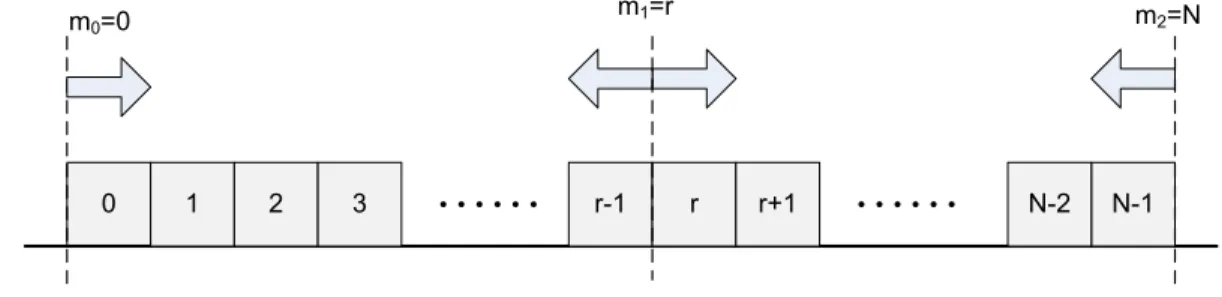
Spectrum fragmentation stems basically from connections with different line rates and the requirement to support mixed line rates in the same network. Hence, connection requests in Flexgrid networks belong to different classes with different spectral requirements. To clarify, we define a class-k request, k = 0, 1, . . . , K − 1, to be one for a spectral block of nk≥ 1 contiguous frequency slots. For example, assuming 6.25 GHz slot width, a 10 Gbps connection requests a spectral block comprising 1 slot only and a 400 Gbps connection requires a contiguous spectral block of 8 slots, both connections using QPSK modulation [20]. This multi-class scenario resembles the multi-service circuit-switched network studied in [21], however it is also very different due to the spectrum continuity and contiguity constraint. In this study, we propose a Class-Based First-Fit (CBFF) spectrum allocation policy with the intention of proactive fragmentation avoidance. In CBFF, the incoming request is placed in the first available spectral block starting from an outset designated for class-k, named as mk, 0 ≤ mk ≤ N − 1, where N is the overall number of frequency slots. If the outset of a class is the left end of the spectrum , i.e., mk = 0, then the search for the first fit is obviously toward the right. If mk = N − 1, then the search for the first fit is toward the left. Otherwise, the search is in both directions and ties are broken randomly. Being computationally simple as its ancestor FF, CBFF gives rise to remarkable performance gains which are shown in several scenarios in the current study including single-hop and network scenarios using simulations.
The organization of the thesis is as follows. The FF and CBFF policies are described in detail in Chapter 2. In Chapter 3, we present simulation re-sults to demonstrate the effectiveness of the proposed spectrum allocation policy CBFF using Poisson connection request arrivals and exponentially distributed connection holding times. The scenarios we consider are i) single-hop scenario ii) NSFNET topology iii) Pan-European network topology. The policies under consideration are i) FF policy ii) CBFF policy. For routing purposes, we study i) Fixed Routing (FR) ii) Fixed Alternate Routing (FAR) with two shortest paths. Finally, we conclude and lay out future research directions of our study.
Chapter 2
First-Fit and Class-Based
First-Fit Spectrum Allocation
Policies
An optical link comprises N contiguous frequency slots, numbered from 0 (the frequency slot at the left end of the spectrum) to N − 1 (the frequency slot at the right end of the spectrum). We have K classes of requests numbered from k = 0 to K −1. A class-k connection requests nkcontiguous slots to be allocated to that connection. For the sake of convenience, we assume n0 < n1 < · · · < nK−1. Let n denote the vector of per-class requests, i.e., n = {n0, n1, . . . , nK−1}. If there is a free spectral block containing nk contiguous frequency slots, then the connection is accepted and one of such free blocks is allocated to the connection. Otherwise, the connection is blocked leading to a non-zero connection blocking probability. If there are multiple free blocks that can satisfy the request, a spectrum allocation policy chooses one from the existing alternatives so as to maximize a certain performance metric. In multi-hop scenarios, the situation is more challenging since a spectral block needs to be free on all the links of the OP that the connection is to use. Not only a desired spectrum allocation policy is to avoid fragmentation on individual links, but it should also give rise to spectral blocks that are free on all links. In CBFF, each class k is associated with a search outset mk, 0 ≤ mk ≤ N ,
for free spectral block search purposes. Note that the outset mk is the boundary between the frequency slots mk−1 and mk. If mk = 0 for some class k, upon a class-k connection request, we start searching from a spectral block starting from slot 0 toward the right. The first free spectral block accommodating the request is allocated to the new connection. The FF policy reduces to mk = 0 for all k since in FF, all connections use the same outset 0. We denote the outset vector of per-class outsets by m, i.e., m = {m0, m1, . . . , mK−1}. As opposed to FF, the CBFF policy uses different outsets for each class mk 6= ml if k 6= l. In particular, our CBFF policy imposes the following. We propose m0 = 0 for class 0 and mK−1 = N − 1. In the latter case, for a connection belonging to class K − 1, we search for a free spectral block toward the left end of the spectrum but starting from the right end. For a class-k connection request 0 < k < K − 1, the outset mk is such that 0 < mk < N − 1 and moreover mk+1 > mk. In this case, the search starts in both directions beginning from outset mk and continues until a free spectral block is found. When two free blocks are found at the same distance from the outset, one of them will be selected randomly. The CBFF policy is depicted in Fig. 2.1 for a Flexgrid optical link with three classes of traffic. Note that in this example the outset for class-1, namely m1, is set to some value r which is the boundary between the frequency slots r − 1 and r.
0 1 2 3 r-1 r r+1 N-2 N-1
m0=0 m2=N
m1=r
Figure 2.1: The CBFF spectrum allocation policy.
Typically, the per-class outsets need to be positioned as far from each other as possible. In case we do not have a-priori knowledge on the input traffic distri-bution, one possibility is to uniformly position the remaining outsets other than 0 and N in the interval [1, N − 1]. In a 3-class system, this policy reduces to positioning the class-1 outset m1 at the mid-point. For example, if K = 3 and
N is even, then m1 = N/2. However, other choices are possible if we know a-priori how the incoming traffic is distributed amongst the traffic classes. For this purpose, let us assume that connection requests arrive at the link with intensity λk and the mean holding time of the accepted connections is 1/µk. The load introduced by class-k connection requests is denoted by ρk:
ρk= nk λk µk
. (2.1)
The overall load is denoted by ρ ρ =
K−1 X
k=0
ρk. (2.2)
The contribution of class-k to the overall load is denoted by αk = ρk/ρ. We propose the following heuristic based on the idea of balancing the load across the spectral blocks between successive per-class outsets. The offered load between successive outsets mi and mi+1 equals to α2i +
αi+1
2 if neither of the points is the left or right end of the spectrum. Mathematically, we have
m1− m0 α0+α21 = mα2− m1 1 2 + α2 2 = · · · = mαK−1K−2 − mK−2 2 + αK−1 (2.3) Since m0 = 0 and mK−1= N , we have K − 2 unknowns with K − 2 linearly inde-pendent equations, the solution of which gives the remaining per-class outsets. In case solutions do not correspond to an integer value, we propose to round them to the nearest integer. Although this outset selection mechanism appears to be provide relatively good results for the singe hop case, its extension to the network case involving multiple links is not straightforward. This difficulty stems from different αk values for different links in the same network. In the current study, we propose to use a single outset vector for all the links in the network based on the entire network demand distribution among multiple classes of connections. Other possibilities are left for future research.
To motivate CBFF, we present the following 3-class example with N = 14 frequency slots in Fig. 2.2. We assume the request vector n = {1, 2, 4}. For CBFF, we use the outset vector m = {0, 7, 14}. We concentrate on a single Flexgrid optical link that is offered with connection requests with the following order: class-0, class-1, class-class-0, class-1, class-class-0, class-1, class-2, class-0. The occupancy diagram
for the optical link after all connection requests are accepted for both FF and CBFF spectrum allocation policies are presented in Fig. 2.2. The fragmentation problem is evident for FF: when any two class-0 connection requests decide to depart, no room will be freed for forthcoming class-1 connections. Similarly, if two class-1 connections decide to leave, there would not be any free spectral block for forthcoming class-2 connection requests. This problem is less problematic with CBFF. If any two successively-arrived class-0 requests decide to leave the link, a spectral block would be freed for a forthcoming class-1 request. Similarly, the departure of both class-1 connections would free room for a class-2 request. Therefore, CBFF favors classes with larger slot requirements whereas FF does not as much. A detailed simulation-study will be presented in the Chapter 3 to quantify the gain achievable by CBFF relative to FF in terms of overall bandwidth blocking rate. 0 1 2 3 4 5 6 7 8 9 0000000000000000000000000000000000000000000000000000000000 0000000000000000000000000000000000000000000000000000000000 0000000000000000000000000000000000000000000000000000000000 0000000000000000000000000000000000000000000000000000000000 0000000000000000000000000000000000000000000000000000000000 0000000000000000000000000000000000000000000000000000000000 0000000000000000000000000000000000000000000000000000000000 0000000000000000000000000000000000000000000000000000000000 0000000000000000000000000000000000000000000000000000000000 0000000000000000000000000000000000000000000000000000000000 0000000000000000000000000000000000000000000000000000000000 10 000000000000000000000000000000000000000000000000000000000 000000000000000000000000000000000000000000000000000000000 000000000000000000000000000000000000000000000000000000000 000000000000000000000000000000000000000000000000000000000 000000000000000000000000000000000000000000000000000000000 000000000000000000000000000000000000000000000000000000000 000000000000000000000000000000000000000000000000000000000 000000000000000000000000000000000000000000000000000000000 000000000000000000000000000000000000000000000000000000000 000000000000000000000000000000000000000000000000000000000 000000000000000000000000000000000000000000000000000000000 11 0 1 2 3 4 5 6 7 8 0000000000000000000000000000000000000000000000000000000000 0000000000000000000000000000000000000000000000000000000000 0000000000000000000000000000000000000000000000000000000000 0000000000000000000000000000000000000000000000000000000000 0000000000000000000000000000000000000000000000000000000000 0000000000000000000000000000000000000000000000000000000000 0000000000000000000000000000000000000000000000000000000000 0000000000000000000000000000000000000000000000000000000000 0000000000000000000000000000000000000000000000000000000000 0000000000000000000000000000000000000000000000000000000000 0000000000000000000000000000000000000000000000000000000000 9 0000000000000000000000000000000000000000000000000000000000 0000000000000000000000000000000000000000000000000000000000 0000000000000000000000000000000000000000000000000000000000 0000000000000000000000000000000000000000000000000000000000 0000000000000000000000000000000000000000000000000000000000 0000000000000000000000000000000000000000000000000000000000 0000000000000000000000000000000000000000000000000000000000 0000000000000000000000000000000000000000000000000000000000 0000000000000000000000000000000000000000000000000000000000 0000000000000000000000000000000000000000000000000000000000 0000000000000000000000000000000000000000000000000000000000 10 000000000000000000000000000000000000000000000000000000000 000000000000000000000000000000000000000000000000000000000 000000000000000000000000000000000000000000000000000000000 000000000000000000000000000000000000000000000000000000000 000000000000000000000000000000000000000000000000000000000 000000000000000000000000000000000000000000000000000000000 000000000000000000000000000000000000000000000000000000000 000000000000000000000000000000000000000000000000000000000 000000000000000000000000000000000000000000000000000000000 000000000000000000000000000000000000000000000000000000000 000000000000000000000000000000000000000000000000000000000 11 Class-0 Class-1 000000000000000000000000000000000000000000 000000000000000000000000000000000000000000 000000000000000000000000000000000000000000 000000000000000000000000000000000000000000 000000000000000000000000000000000000000000 000000000000000000000000000000000000000000 000000000000000000000000000000000000000000 000000000000000000000000000000000000000000 Class-2 a) FF Policy b) CBFF Policy m={0,7,14} n={1,2,4} 0000000000000000000000000000000000000000000000000000000000 0000000000000000000000000000000000000000000000000000000000 0000000000000000000000000000000000000000000000000000000000 0000000000000000000000000000000000000000000000000000000000 0000000000000000000000000000000000000000000000000000000000 0000000000000000000000000000000000000000000000000000000000 0000000000000000000000000000000000000000000000000000000000 0000000000000000000000000000000000000000000000000000000000 0000000000000000000000000000000000000000000000000000000000 0000000000000000000000000000000000000000000000000000000000 0000000000000000000000000000000000000000000000000000000000 12 0000000000000000000000000000000000000000000000000000000000 0000000000000000000000000000000000000000000000000000000000 0000000000000000000000000000000000000000000000000000000000 0000000000000000000000000000000000000000000000000000000000 0000000000000000000000000000000000000000000000000000000000 0000000000000000000000000000000000000000000000000000000000 0000000000000000000000000000000000000000000000000000000000 0000000000000000000000000000000000000000000000000000000000 0000000000000000000000000000000000000000000000000000000000 0000000000000000000000000000000000000000000000000000000000 0000000000000000000000000000000000000000000000000000000000 13 0000000000000000000000000000000000000000000000000000000000 0000000000000000000000000000000000000000000000000000000000 0000000000000000000000000000000000000000000000000000000000 0000000000000000000000000000000000000000000000000000000000 0000000000000000000000000000000000000000000000000000000000 0000000000000000000000000000000000000000000000000000000000 0000000000000000000000000000000000000000000000000000000000 0000000000000000000000000000000000000000000000000000000000 0000000000000000000000000000000000000000000000000000000000 0000000000000000000000000000000000000000000000000000000000 0000000000000000000000000000000000000000000000000000000000 12 0000000000000000000000000000000000000000000000000000000000 0000000000000000000000000000000000000000000000000000000000 0000000000000000000000000000000000000000000000000000000000 0000000000000000000000000000000000000000000000000000000000 0000000000000000000000000000000000000000000000000000000000 0000000000000000000000000000000000000000000000000000000000 0000000000000000000000000000000000000000000000000000000000 0000000000000000000000000000000000000000000000000000000000 0000000000000000000000000000000000000000000000000000000000 0000000000000000000000000000000000000000000000000000000000 0000000000000000000000000000000000000000000000000000000000 13
Figure 2.2: Illustration of the FF and CBFF spectrum allocation policies for a 3-class numerical example.
Chapter 3
Experiment Results
3.1
Simulator
A simulator is developed using Java programming language to test the proposed spectrum allocation policies for dynamic Flexgrid optical networks. The simulator is developed so that different topologies and traffic profiles can be tested. The simulator first creates the nodes and edges of the network based on the given connection matrix that defines the network topology. One or two shortest paths, depending on whether FR or FAR is used, are calculated from each node to every other node using Dijkstra’s algorithm. The per-class connection request traffic is assumed to be Poisson with intensity λk and accepted connections’ holding times are exponentially distributed with mean 1/µk. Hence, traffic information is provided in terms of arrival rate matrices and mean holding time matrices for each class. Simulation type is chosen to be event-driven to achieve results closer to practical ones. A priority-queue data structure is utilized for this purpose. Only the closest arrivals at every path is known at a given time, which are prioritized depending on the event-times. The simulator processes existing connections till the closest request. After terminating the expired connections, it allocates the request based on the given spectrum assignment policy, FF or CBFF. When using FR, if no available spectrum is found for the request, it is dropped. On the other
hand, FAR provides a second path for the request to be allocated. The request is dropped if it can be allocated to neither. All allocations and dropped requests are recorded for evaluation. The simulation results are then exported to MATLAB environment for processing.
Of greater importance, throughput for a given blocking probability is investi-gated. Towards the intention of providing valuable insight on the fragmentation problem, such as its causes and which traffic profiles suffer most from fragmen-tation, each class of requests are studied in terms of their blocking probabilities. A number of setups are created to get experimental results. For simplicity, Poisson connection arrival process and exponential connection holding times are assumed without the loss of generality. The link capacities are set to 128 slots. Simulation times are set to 107seconds to guarantee validity of experiments. Each experiment is made with three classes of requests based on their required number of slots. For each setup, 5 different traffic profiles are simulated and analyzed.
3.2
Presentation Methodology
Three types of graphs are prepared for each profile: total bandwidth blocking probability vs. arrival rate; per-class blocking probability vs. arrival rate; and throughput vs. blocking probability. Total number of connection requests by class kth class is assumed to be Θk. Number of blocked connection requests out of Θk requests is θk. The per-class blocking probability, Pk, is calculated as in Equation 3.1.
Pk= θk Θk
(3.1)
In order to calculate the total requested bandwidth, denoted by Θ, the number of requests from each class should be added after being multiplied by the number of slots required for that request. Equation 3.2 and Equation 3.3 demonstrate the calculation of total requested bandwidth Θ and the total bandwidth of blocked
requests θ, respectively. Θ = K−1 X k=0 nkΘk (3.2) θ = K−1 X k=0 nkθk (3.3)
The overall bandwidth blocking probability PBis calculated as in Equation 3.4 by dividing the total blocked bandwidth request θ by the total bandwidth request made Θ.
PB = θ
Θ (3.4)
In order to provide more insight on the effectiveness of CBFF against the FF policy, we introduce the so-called throughput, denoted by T (PB), is the max-imum rate of slot requests that are accepted not exceeding a certain desired bandwidth blocking probability PB. Throughput parameter T (PB) is calculated as in Equation 3.5 where λk(PB) denotes the per-class-k arrival rate at which the overall blocking probability PB is realized. The percentage increase in throughput (∆T(PB)) introduced in Equation 3.6 is indicative of how much spectral resources are wasted in FF compared to CBFF when a desired bandwidth blocking proba-bility of PB is realized. T (PB) = ( X k λk(PB)nk)(1 − PB) (3.5) ∆T(PB) = 100 TCBF F(P B) − TF F(PB) TF F(P B) (3.6)
3.3
Single Link Setup
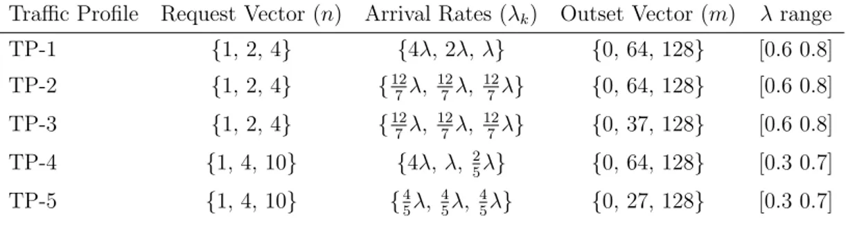
In the first setup, a two-node, single-link network is used. The network topology is seen on Figure 3.1. In this setup, FF and CBFF policies are compared for the single-hop scenario. Moreover, the impact of outset vector selection on the effectiveness of CBFF is investigated. Five traffic profiles(TP) are used for this setup. Among traffic profiles, relative arrival rates of classes are changed. More-over, outsets of classes are varied for the CBFF algorithm. Table 3.1 explains the details of these traffic profiles. Since this is a single-hop scenario, only one routing solution exists which is FR in this case.
Figure 3.1: Single Link Topology
Traffic Profile Request Vector (n) Arrival Rates (λk) Outset Vector (m) λ range
TP-1 {1, 2, 4} {4λ, 2λ, λ} {0, 64, 128} [0.6 0.8] TP-2 {1, 2, 4} {12 7λ, 12 7λ, 12 7λ} {0, 64, 128} [0.6 0.8] TP-3 {1, 2, 4} {12 7λ, 12 7λ, 12 7λ} {0, 37, 128} [0.6 0.8] TP-4 {1, 4, 10} {4λ, λ, 2 5λ} {0, 64, 128} [0.3 0.7] TP-5 {1, 4, 10} {4 5λ, 4 5λ, 4 5λ} {0, 27, 128} [0.3 0.7]
Table 3.1: Single Link Setup
First of all, note that although the contribution of each class to overall load changes, the total load is kept constant by manipulating arrival rates. The λ coefficient is swept through the range with steps of 0.001 to get fine results. Ranges are chosen to correspond to an overall bandwidth blocking probability range of 10−5 to 10−1. The arrival rate matrix for each class k is constructed as in Equation 3.7 where the i, j th entry gives the connection arrival rate from node i to node j for class k. Similarly, the mean holding time matrix for each class is assumed to be fixed over classes as in Equation 3.8.
Λk= " 0 λk λk 0 # (3.7)
Mk= " 0 0.1 0.1 0 # (3.8)
TP-1 has balanced load distribution between classes and outsets are chosen according to Equation 2.3. In TP-2, instead of having balanced load distributions, equal arrival rates for the three classes is studied with outsets not chosen according to Equation 2.3. TP-3 differs from TP-2 in only the selection of outsets since it uses Equation 2.3. Comparing the results of TP-2 and TP-3, the effect of outset vector selection on the CBFF policy will be studied. TP-4 and TP-5 are chosen with classes represented by a different request vector n = {1, 4, 10}. It is conjectured that when the gap between class sizes are increased, the FF algorithm would suffer more from fragmentation. Therefore, CBFF supposedly will do much better for scenarios with classes with larger size gaps.
3.4
Single Link Results
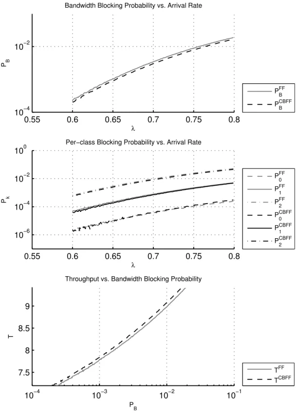
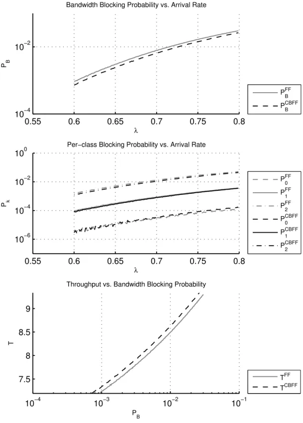
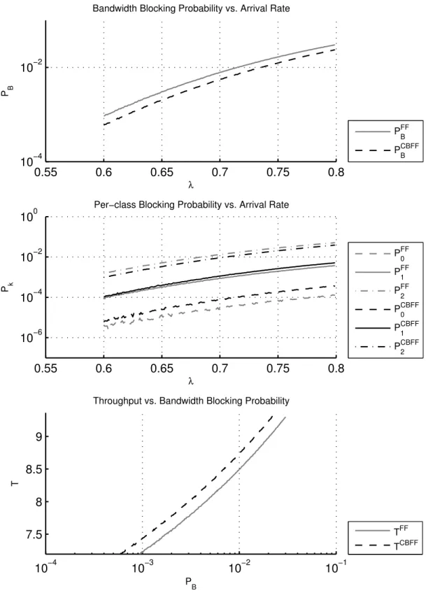
The first graph for each profile, bandwidth blocking probability vs. arrival rate, represents one of the most important outcomes of our study. Achieving lower bandwidth blocking probability under the same traffic conditions is very desir-able. This graph compares overall bandwidth blocking probabilities achieved under FF and CBFF policies. The second graph, per-class blocking probability vs. arrival rate, gives a valuable insight on how a better blocking probability is achieved and how the policies affect different classes. Last but not least, the third graph, throughput vs. blocking probability, is also one of the most important out-comes in summarizing the overall performance of alternative spectrum allocation policies. This graph makes it easy to see how much spectral resources are wasted. It is desirable to handle more traffic (increased throughput) without sacrificing quality of service which is measured by overall bandwidth blocking probability. Throughput is directly proportional to offered load and therefore to utilization of spectral resources. Figures 3.2, 3.3, 3.4, 3.5 and 3.6 present the results for TP-1, TP-2, TP-3 TP-4 and TP-5, which are described in Table 3.1, respectively.
0.55 0.6 0.65 0.7 0.75 0.8 10−4
10−2
Bandwidth Blocking Probability vs. Arrival Rate
λ P B PFF B PCBFF B 0.55 0.6 0.65 0.7 0.75 0.8 10−6 10−4 10−2 100
Per−class Blocking Probability vs. Arrival Rate
λ P k PFF 0 PFF 1 PFF 2 PCBFF 0 PCBFF 1 PCBFF 2 10−4 10−3 10−2 10−1 7.5 8 8.5 9
Throughput vs. Bandwidth Blocking Probability
P
B
T
TFF TCBFF
0.2 0.3 0.4 0.5 0.6 0.7 10−6
10−4 10−2
Bandwidth Blocking Probability vs. Arrival Rate
λ P B PFF B PCBFF B 0.2 0.3 0.4 0.5 0.6 0.7 10−6 10−4 10−2 100
Per−class Blocking Probability vs. Arrival Rate
λ P k PFF 0 PFF 1 PFF 2 PCBFF 0 PCBFF 1 PCBFF 2 10−6 10−4 10−2 4 5 6 7 8
Throughput vs. Bandwidth Blocking Probability
P
B
T
TFF TCBFF
0.2 0.3 0.4 0.5 0.6 0.7 10−6
10−4 10−2
Bandwidth Blocking Probability vs. Arrival Rate
λ P B PFF B PCBFF B 0.2 0.3 0.4 0.5 0.6 0.7 10−6 10−4 10−2 100
Per−class Blocking Probability vs. Arrival Rate
λ P k PFF 0 PFF 1 PFF 2 PCBFF 0 PCBFF 1 PCBFF 2 10−6 10−4 10−2 4 5 6 7
Throughput vs. Bandwidth Blocking Probability
P
B
T
TFF TCBFF
First of all, the blocking probability vs. arrival rate graphs show that CBFF performs better in terms of overall bandwidth blocking probability, namely up to 0.02. Therefore CBFF increases spectral efficiency. By closely investigating the per-class blocking probability vs. lambda graphs, it is first noted that CBFF increases blocking probability of class-0 (P0) for all profiles. This however, is an expected result. Note that class-0 is the one class that does not suffer from fragmentation. Since it requires only one frequency slot, its dropping is solely due to lack of bandwidth resources. When CBFF is used, it reduces fragmentation, therefore more requests belonging to classes with larger IDs are accepted into the link. This in turn reduces spectral resources left for the first class, causing increased drop rate for that particular class. This is a natural outcome of the algorithm. The class-2 is the class that most benefits from the use of CBFF. Since other classes are more valuable than the first class in terms of spectral resources, overall bandwidth blocking probability is reduced.
Bandwidth blocking probability vs. arrival rate graphs also show that the improvement on bandwidth blocking probability decreases with increasing load. This is because CBFF improves bandwidth blocking probability by reducing frag-mentation. However, after a certain amount of load is offered to the network, the blocking probability is mostly due to lack of spectral resources. The point where improvement introduced by CBFF considerably drops is well outside practical operating limits. Likewise when there is very low load on network, fragmentation becomes less effective on bandwidth blocking probability. Under very low loads, no blocking is seen, regardless of the allocation policy. CBFF shows its effect when the network is fairly loaded and fragmentation problem is apparent.
Another important result can be derived from the single link setup by exam-ining Figures 3.3 and 3.4. The only difference between these profiles is the choice of the outset for class-1. In TP-2, m1 is set in the middle. In TP-3 however, the outset vector is set according to Equation 2.3. Increase in throughput in TP-2 is between 1.57 − 1.56%, whereas TP-3 achieves an 2.95 − 2.84% increase. For the single link setup, it is seen that throughput is increased up to 7.68%.
the single link setup, Table 3.2 summarizes the percentage increase in throughput (∆T) which is calculated by Equation 3.6. Note that the throughout increase varies with respect to different bandwidth blocking probabilities. Corresponding bandwidth blocking probability ranges are also given in Table 3.2.
Traffic Profile BW Blocking Prob. Range Throughput Increase (%) (∆T)
TP-1 10−3− 10−1 1.04 - 0.76
TP-2 10−3− 10−1 1.57 - 1.56
TP-3 10−3− 10−1 2.96 - 2.84
TP-4 10−3− 10−1 3.10 - 2.83
TP-5 10−3− 10−1 7.68 - 6.30
Table 3.2: Single Link Setup Improvement with CBFF
TP-5 has constant arrival rates for each class. Therefore, contribution of the largest class to the traffic is higher. Also, in TP-5, n = 1, 4, 10 rather than n = 1, 2, 4. This makes TP-5 most vulnerable to fragmentation problems because n2 = 10 and contribution of class-2 to overall load is greater. Since CBFF increases spectral efficiency by alleviating fragmentation, TP-5 shows the most increase in throughput according to Table 3.2.
3.5
Realistic Setups
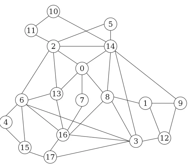
In second setup, NSF Network and PAN-European Network topologies are used. Figure 3.7 and Figure 3.8 show these topologies respectively.
Figure 3.7: NSF Network Topology
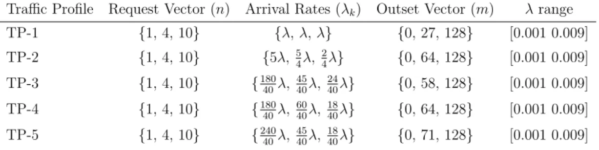
Five different traffic profiles are tested with this setup. In all profiles, outsets are chosen according to Equation 2.3. While overall load remains the same, TP-1 assumes fixed arrival rates for each class. TP-2 utilizes fixed load contribution from each class. TP-3 favors class-2 such as its contribution to overall load is 40% while other two classes has 30% contribution each. TP-4 and TP-5 favor class-1 and class-0 respectively. Table 3.3 explains these traffic profiles in detail. These 5 traffic profiles are simulated under both FR and FAR(2 shortest paths) algorithms.
Traffic Profile Request Vector (n) Arrival Rates (λk) Outset Vector (m) λ range
TP-1 {1, 4, 10} {λ, λ, λ} {0, 27, 128} [0.001 0.009] TP-2 {1, 4, 10} {5λ, 5 4λ, 2 4λ} {0, 64, 128} [0.001 0.009] TP-3 {1, 4, 10} {180 40λ, 45 40λ, 24 40λ} {0, 58, 128} [0.001 0.009] TP-4 {1, 4, 10} {180 40λ, 60 40λ, 18 40λ} {0, 64, 128} [0.001 0.009] TP-5 {1, 4, 10} {240 40λ, 45 40λ, 18 40λ} {0, 71, 128} [0.001 0.009]
Table 3.3: Realistic Setup (NSF Net and PAN-Eur Net)
Again, lambda ranges are chosen to cover overall bandwidth blocking prob-ability range of 10−5 to 10−1. The arrival rate λ is swept through the range
Figure 3.8: PAN-European Network Topology
with 0.00025 steps. Note that the arrival rate matrix for each class is defined in Equation 3.9 by its i, jth element and travel requests on every route is assumed to be uniformly distributed. Mean holding time matrix for each class is defined in Equation 3.10 by its i, jth element also. It is fixed for each class and route. The sizes of arrival rate matrices and mean holding time matrices depend on the topology since they cover each possible path on the topologies.
Λi,jk = λk if i 6= j 0 if i = j (3.9)
Mki,j = 0.01 if i 6= j 0 if i = j (3.10)
3.6
NSF Network Results
Figures 3.9, 3.10, 3.11, 3.12 and 3.13 present the results for TP-1, TP-2, TP-3 TP-4 and TP-5, respectively, with FAR as the routing algorithm. Fig-ures 3.14, 3.15, 3.16, 3.17 and 3.18 present the results for TP-1, TP-2, TP-3, TP-4, and TP-5, respectively, with FR as the routing algorithm.
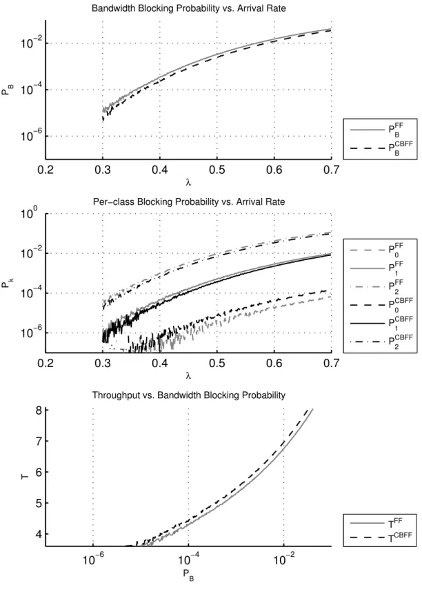
Since the class with largest size suffers most from fragmentation in FF algo-rithm, it is predicted that when the class-2 is favored in these profiles, namely TP-1 and TP-3, CBFF’s performance improvement will be more significant. Band-width blocking probability vs. arrival rate graphs show that blocking probability is decreased compared to that of FF algorithm at all traffic profiles. Therefore CBFF improves spectral utilization for the realistic NSF Network as well. When bandwidth blocking probability vs. arrival rate and throughput vs. bandwidth blocking probability graphs in Figure 3.11 is closely investigated, although CBFF does better, the conclusion that performance of FF and CBFF gets closer at very low and very high loads becomes much more clear. It is seen that the block-ing probabilities get closer at arrival rate (λ) values around 2.10−3 and 8.10−3, which correspond to overall bandwidth blocking probability of 10−7 and 10−1, respectively.
2 4 6 8 10 x 10−3 10−6 10−4 10−2 100
Bandwidth Blocking Probability vs. Arrival Rate
λ P B PFF B PCBFF B 2 4 6 8 10 x 10−3 10−6 10−4 10−2 100
Per−class Blocking Probability vs. Arrival Rate
λ P k PFF 0 PFF 1 PFF 2 PCBFF 0 PCBFF 1 PCBFF 2 10−6 10−4 10−2 100 0.04 0.06 0.08 0.1
Throughput vs. Bandwidth Blocking Probability
P
B
T
TFF TCBFF
2 4 6 8 10 x 10−3 10−6 10−4 10−2 100
Bandwidth Blocking Probability vs. Arrival Rate
λ P B PFF B PCBFF B 2 4 6 8 10 x 10−3 10−6 10−4 10−2 100
Per−class Blocking Probability vs. Arrival Rate
λ P k PFF 0 PFF 1 PFF 2 PCBFF 0 PCBFF 1 PCBFF 2 10−6 10−4 10−2 100 0.04 0.06 0.08 0.1 0.12
Throughput vs. Bandwidth Blocking Probability
P
B
T
TFF TCBFF
2 4 6 8 10 x 10−3 10−6 10−4 10−2 100
Bandwidth Blocking Probability vs. Arrival Rate
λ P B PFF B PCBFF B 2 4 6 8 10 x 10−3 10−6 10−4 10−2 100
Per−class Blocking Probability vs. Arrival Rate
λ P k PFF 0 PFF 1 PFF 2 PCBFF 0 PCBFF 1 PCBFF 2 10−6 10−4 10−2 100 0.04 0.06 0.08 0.1
Throughput vs. Bandwidth Blocking Probability
P B T TFF TCBFF Figure 3.14: FR, NSFNET TP-1
2 4 6 8 10 x 10−3 10−6 10−4 10−2 100
Bandwidth Blocking Probability vs. Arrival Rate
λ P B PFF B PCBFF B 2 4 6 8 10 x 10−3 10−6 10−4 10−2 100
Per−class Blocking Probability vs. Arrival Rate
λ P k PFF 0 PFF 1 PFF 2 PCBFF 0 PCBFF 1 PCBFF 2 10−6 10−4 10−2 100 0.04 0.06 0.08 0.1
Throughput vs. Bandwidth Blocking Probability
P B T TFF TCBFF Figure 3.15: FR, NSFNET TP-2
2 4 6 8 10 x 10−3 10−6 10−4 10−2 100
Bandwidth Blocking Probability vs. Arrival Rate
λ P B PFF B PCBFF B 2 4 6 8 10 x 10−3 10−6 10−4 10−2 100
Per−class Blocking Probability vs. Arrival Rate
λ P k PFF 0 PFF 1 PFF 2 PCBFF 0 PCBFF 1 PCBFF 2 10−6 10−4 10−2 100 0.04 0.06 0.08 0.1
Throughput vs. Bandwidth Blocking Probability
P B T TFF TCBFF Figure 3.16: FR, NSFNET TP-3
2 4 6 8 10 x 10−3 10−6 10−4 10−2 100
Bandwidth Blocking Probability vs. Arrival Rate
λ P B PFF B PCBFF B 2 4 6 8 10 x 10−3 10−6 10−4 10−2 100
Per−class Blocking Probability vs. Arrival Rate
λ P k PFF 0 PFF 1 PFF 2 PCBFF 0 PCBFF 1 PCBFF 2 10−6 10−4 10−2 100 0.04 0.06 0.08 0.1
Throughput vs. Bandwidth Blocking Probability
P B T TFF TCBFF Figure 3.17: FR, NSFNET TP-4
2 4 6 8 10 x 10−3 10−6 10−4 10−2 100
Bandwidth Blocking Probability vs. Arrival Rate
λ P B PFF B PCBFF B 2 4 6 8 10 x 10−3 10−6 10−4 10−2 100
Per−class Blocking Probability vs. Arrival Rate
λ P k PFF 0 PFF 1 PFF 2 PCBFF 0 PCBFF 1 PCBFF 2 10−6 10−4 10−2 100 0.04 0.06 0.08 0.1
Throughput vs. Bandwidth Blocking Probability
P B T TFF TCBFF Figure 3.18: FR, NSFNET TP-5
Table 3.4 summarizes the results of simulations for the NSF Network under the FAR algorithm and Table 3.5 summarizes the results of those under the FR algorithm. We observe that for the constant lambda profile, TP-1, benefits of CBFF are remarkable. An increase of up to 12.59% throughput is achieved with the CBFF algorithm relative to FF. This is again due to the fact that CBFF reduces fragmentation and fragmentation is more effective for larger classes. Since in TP-1 all classes have the same arrival rate, the contribution of the largest class to overall traffic is largest. By reducing its blocking probability, the overall bandwidth blocking probability can be greatly improved. For more balanced traffic profiles, namely TP-2 to TP-5, a waste of approximately 6% is eliminated by the use of CBFF. As predicted, TP-1 and TP-3 are the profiles that most benefit from CBFF, which is evident by ∆T values at 10−1 blocking probability in Tables 3.4 and 3.5. CBFF introduces improvement when used with both FR and FAR. Improvements in throughput under either routing algorithm is very close.
Traffic Profile BW Blocking Prob. Range Throughput Increase (%) (∆T)
TP-1 10−5− 10−1 12.59 - 10.47
TP-2 10−5− 10−1 6.31 - 4.35
TP-3 10−5− 10−1 5.13 - 4.47
TP-4 10−5− 10−1 5.25 - 4.17
TP-5 10−5− 10−1 6.76 - 3.31
Table 3.4: FAR, NSF Network Setup Improvement with CBFF Traffic Profile BW Blocking Prob. Range Throughput Increase (%) (∆T)
TP-1 10−5− 10−1 12.30 - 10.23
TP-2 10−5− 10−1 6.03 - 3.98
TP-3 10−5− 10−1 5.25 - 4.27
TP-4 10−5− 10−1 6.31 - 4.07
TP-5 10−5− 10−1 7.08 - 3.16
3.7
PAN-European Network Results
Same traffic profiles as NSFNET are used in the PAN-European Network which is a more dense network than NSF. Figures 3.19, 3.20, 3.21, 3.22 and 3.23 present the results for TP-1, TP-2, TP-3, TP-4, and TP-5, under the FAR algorithm and Figures 3.24, 3.25, 3.26, 3.27 and 3.28 present the results for those under the FR algorithm, respectively.
Similar effects to that of the NSF Network case is observable in this setup too. It is again most clear in Figure 3.21 that the performances of FF and CBFF get closer at low and high load cases. Class-0 is again unfavored because of the fact that it just does not suffer from fragmentation.
1 2 3 4 5 6 7 8 x 10⁻³ 10−6 10−4 10−2 100
Bandwidth Blocking Probability vs. Arrival Rate
λ P B PFF B PCBFF B 1 2 3 4 5 6 7 8 x 10⁻³ 10−6 10−4 10−2 100
Per−class Blocking Probability vs. Arrival Rate
λ P k PFF 0 PFF 1 PFF 2 PCBFF 0 PCBFF 1 PCBFF 2 10−6 10−4 10−2 100 0.02 0.04 0.06 0.08 0.1
Throughput vs. Bandwidth Blocking Probability
P
B
T
TFF TCBFF
2 3 4 5 6 7 8 x 10⁻³ 10−6 10−4 10−2 100
Bandwidth Blocking Probability vs. Arrival Rate
λ P B PFF B PCBFF B 2 3 4 5 6 7 8 x 10⁻³ 10−6 10−4 10−2 100
Per−class Blocking Probability vs. Arrival Rate
λ P k PFF 0 PFF 1 PFF 2 PCBFF 0 PCBFF 1 PCBFF 2 10−6 10−4 10−2 100 0.02 0.04 0.06 0.08 0.1
Throughput vs. Bandwidth Blocking Probability
P
B
T
TFF TCBFF
Table 3.6 and Table 3.7 summarize the results of the PAN-European Network setup under FAR and FR algorithms, respectively. Again a substantial increase of 15.79% in throughput is seen in TP-1, which has constant lambdas meaning class-2 (n2 = 10) is most favored. Again, TP-1 and TP-3 benefits most by the use of CBFF since the two favors class-2 in terms of contribution to overall traffic. TP-2 to TP-5 shows an increase of approximately 6% to 8% on throughput with the help of CBFF algorithm. Again, it can be concluded that CBFF improves throughput under both FAR and FR algorithms.
Traffic Profile BW Blocking Prob. Range Throughput Increase (%) (∆T)
TP-1 10−5− 10−1 14.79 - 11.22
TP-2 10−5− 10−1 7.59 - 3.55
TP-3 10−5− 10−1 7.08 - 4.17
TP-4 10−5− 10−1 6.17 - 3.55
TP-5 10−5− 10−1 6.31 - 2.40
Table 3.6: FAR, PAN-European Network Setup Improvement with CBFF Traffic Profile BW Blocking Prob. Range Throughput Increase (%) (∆T)
TP-1 10−5− 10−1 12.30 - 10.23
TP-2 10−5− 10−1 11.75 - 2.00
TP-3 10−5− 10−1 6.47 - 3.55
TP-4 10−5− 10−1 6.31 - 2.00
TP-5 10−5− 10−1 5.01 - 2.00
Chapter 4
Conclusions
We have proposed a novel policy called Class-Based First Fit algorithm (CBFF) for the spectrum allocation problem component of the general routing and spec-trum allocation (RSA) problem that arises in Flexgrid optical networks under dynamic traffic conditions. The proposed CBFF policy enhances spectral uti-lization by reducing fragmentation. The CBFF policy attempts to alleviate the fragmentation problem in elastic optical networks by clustering connection re-quests together that request the same number of frequency slots. This policy naturally favors connection requests demanding larger number of frequency slots. Since more spectral resources are allocated to these requests, connection requests demanding fewer frequency slots may be slightly penalized. However, we have shown through exhaustive simulations that CBFF decreases overall bandwidth blocking probability and increases throughput up to around 15%.
The proposed algorithm is only studied with the assumption of Poisson arrival rates and exponentially distributed connection holding times. A potential future research topic is the exploration of CBFF under more general traffic patterns and to more general network topologies and with larger link capacities. Moreover, a constant outset vector for the CBFF policy is used for all links of the network that is based on the incoming traffic distribution. Rather than depending on static traffic parameterization, the load on each link can be simultaneously monitored and the outset vector can be dynamically changed for each path. We tend to
believe that if these outsets are dynamically changed throughout the simulations and can be changed for each path separately, the improvement introduced by CBFF policy may be enhanced. Since a number of paths use common links, an-other optimization problem is introduced when each link is assigned to a different outset vector. Solving this optimization problem can be another enhancement to the practical implementation of the CBFF policy. Also, since the idea behind setting outsets is to separate each class as far as possible, another algorithm may be used for setting outsets with separation of classes kept in mind.
Bibliography
[1] E. Pincemin, “Challenges of 40/100 gbps deployments in long-haul transport networks on existing fibre and system infrastructure,” in Optical Fiber Com-munication (OFC), collocated National Fiber Optic Engineers Conference, 2010 Conference on (OFC/NFOEC), pp. 1–3, 2010.
[2] O. Gerstel, M. Jinno, A. Lord, and S. J. B. Yoo, “Elastic optical network-ing: a new dawn for the optical layer?,” Communications Magazine, IEEE, vol. 50, no. 2, pp. s12–s20, 2012.
[3] M. Jinno, H. Takara, B. Kozicki, Y. Tsukishima, Y. Sone, and S. Mat-suoka, “Spectrum-efficient and scalable elastic optical path network: archi-tecture, benefits, and enabling technologies,” Communications Magazine, IEEE, vol. 47, no. 11, pp. 66–73, 2009.
[4] M. Jinno, B. Kozicki, H. Takara, A. Watanabe, Y. Sone, T. Tanaka, and A. Hirano, “Distance-adaptive spectrum resource allocation in spectrum-sliced elastic optical path network [topics in optical communications],” Com-munications Magazine, IEEE, vol. 48, no. 8, pp. 138–145, 2010.
[5] P. Gambini, M. Renaud, C. Guillemot, F. Callegati, I. Andonovic, B. Bostica, D. Chiaroni, G. Corazza, S. L. Danielsen, P. Gravey, P. B. Hansen, M. Henry, C. Janz, A. Kloch, R. Krahenbuhl, C. Raffaelli, M. Schilling, A. Talneau, and L. Zucchelli, “Transparent optical packet switching: network architecture and demonstrators in the KEOPS project,” JSAC, vol. 16, pp. 1245–1259, 1998.
[6] C. Qiao and M. Yoo, “Optical burst switching (OBS) - a new paradigm for an optical Internet,” Jour. High Speed Networks (JHSN), vol. 8, no. 1, pp. 69–84, 1999.
[7] L. Xu, H. Perros, and G. Rouskas, “Techniques for optical packet switch-ing and optical burst switchswitch-ing,” IEEE Communications Magazine, vol. 39, pp. 136 –142, jan 2001.
[8] L. Velasco, M. Klinkowski, M. Ruiz, and J. Comellas, “Modeling the routing and spectrum allocation problem for flexgrid optical networks,” Photonic Network Communications, vol. 24, no. 3, pp. 177–186, 2012.
[9] P. Wright, A. Lord, and L. Velasco, “The network capacity benefits of Flex-grid,” in Optical Network Design and Modeling (ONDM), 2013 17th Inter-national Conference on, pp. 7–12, 2013.
[10] K. Christodoulopoulos, I. Tomkos, and E. A. Varvarigos, “Elastic bandwidth allocation in flexible ofdm-based optical networks,” IEEE/OSA Journal of Lightwave Technology, vol. 29, pp. 1354–1366, May 2011.
[11] Y. Wang, X. Cao, and Y. Pan, “A study of the routing and spectrum alloca-tion in spectrum-sliced elastic optical path networks,” in INFOCOM, 2011 Proceedings IEEE, pp. 1503–1511, 2011.
[12] Y. Wang, J. Zhang, Y. Zhao, J. Wang, and W. Gu, “Routing and spec-trum assignment by means of ant colony optimization in flexible band-width networks,” in Optical Fiber Communication Conference and Expo-sition (OFC/NFOEC), 2012 and the National Fiber Optic Engineers Con-ference, pp. 1–3, 2012.
[13] K. Christodoulopoulos, I. Tomkos, and E. Varvarigos, “Routing and spec-trum allocation in ofdm-based optical networks with elastic bandwidth al-location,” in Global Telecommunications Conference (GLOBECOM 2010), 2010 IEEE, 2010.
[14] A. Rosa, C. Cavdar, S. Carvalho, J. Costa, and L. Wosinska, “Spectrum allocation policy modeling for elastic optical networks,” in High Capacity
Optical Networks and Enabling Technologies (HONET), 2012 9th Interna-tional Conference on, pp. 242–246, 2012.
[15] X. Wang, Q. Zhang, I. Kim, P. Palacharla, and M. Sekiya, “Utilization entropy for assessing resource fragmentation in optical networks,” in Optical Fiber Communication Conference and Exposition (OFC/NFOEC), 2012 and the National Fiber Optic Engineers Conference, 2012.
[16] X. Yu, J. Zhang, Y. Zhao, T. Peng, Y. Bai, D. Wang, and X. Lin, “Spectrum compactness based defragmentation in flexible bandwidth optical networks,” in Optical Fiber Communication Conference and Exposition (OFC/NFOEC), 2012 and the National Fiber Optic Engineers Conference, 2012.
[17] Y. Wang, J. Zhang, Y. Zhao, J. Liu, and W. Gu, “Spectrum consecutive-ness based routing and spectrum allocation in flexible bandwidth networks,” Chinese Optics Letters, pp. S10606 1–4, 2012.
[18] E. Karasan and E. Ayanoglu, “Effects of wavelength routing and selection algorithms on wavelength conversion gain in wdm optical networks,” Net-working, IEEE/ACM Transactions on, vol. 6, no. 2, pp. 186–196, 1998. [19] X. Sun, Y. Li, I. Lambadaris, and Y. Zhao, “Performance analysis of first-fit
wavelength assignment algorithm in optical networks,” in Telecommunica-tions, 2003. ConTEL 2003. Proceedings of the 7th International Conference on, vol. 2, pp. 403–409 vol.2, 2003.
[20] A. Castro, L. Velasco, M. Ruiz, M. Klinkowski, J. P. Fern´andez-Palacios, and D. Careglio, “Dynamic routing and spectrum (re) allocation in future flexgrid optical networks,” Computer Networks, vol. 56, no. 12, pp. 2869– 2883, 2012.
[21] K. W. Ross, Multiservice Loss Models for Broadband Telecommunication Net-works. Secaucus, NJ, USA: Springer-Verlag New York, Inc., 1995.