Full Length Research Paper
Solving a system of nonlinear fractional partial
differential equations using three dimensional
differential transform method
Muhammet Kurulay
1, Bayram Ali Ibrahimo lu
2*and Mustafa Bayram
31Department of Mathematics, Faculty of Art and Sciences, Yildiz Technical University 34210-Davutpasa- stanbul, Turkey.
2Mathematical Engineering Department, Yildiz Technical University, 34210-Davutpasa- stanbul, Turkey. 3Department of Mathematics, Faculty of Arts and Science, Fatih Universty, 34500 Büyükçekmece, Istanbul, Turkey.
Accepted 06 April, 2010
In this article, three dimensional fractional partial differential transform method (FPDTM) has been employed to obtain solutions of a System of nonlinear fractional partial differential equations. This indicates the validity and great potential of the homotopy analysis method for solving system of fractional partial differential equations. Fractional differential transform method can easily be applied to nonlinear problems and reduces the size of computational work. With this method exact solutions may be obtained without any need of cumbersome work and it is a useful tool for analytical and numerical solutions. The fractional derivative is described in the caputo sense.
Key words: Fractional partial differential transform method, Caputo fractional derivative, system of fractional partial differential equations.
INTRODUCTION
Mathematical modeling of many physical systems leads to linear and nonlinear fractional differential equations in various fields of physics and engineering. The numerical and analytical approximations of such systems have been intensively studied since the work of Padovan (1987). Recently, several mathematical methods including the Adomian decomposition method (Hosseini and Jafari, 2009; Lei Wu et al., 2009) variational iteration method (Noor et al., 2008; Odibat and Momani, 2006) homotopy perturbation method (Jafari and Seifi., 2009; Hang Xu et al., 2009) and fractional difference method (Podlubny, 1999) have been developed to obtain exact and approximate analytic solutions. Some of these methods use transformation in order to reduce equations into simpler equations or systems of equations and some other methods give the solution in a series form which converges to the exact solution. Among these solution techniques, the variational iteration method and the Adomian decomposition method are the most clear
*Corresponding author. E-mail: [email protected]
methods of solution of fractional differential and integral equations, because they provide immediate and visible symbolic terms of analytic solutions, as well as numerical approximate solutions to both linear and nonlinear differential equations without linearization or discretization.
In the last decades, fractional calculus has found diverse applications in various scientific and technological fields (Podlubny, 1999; Hilfer, 1999), such as thermal engineering, acoustics, fluid mechanics, biology, chemistry, electromagnetism, control, robotics, viscoelas-ticity, diffusion, edge detection, turbulence, signal processing and many other physical processes.
The differential transform method was first applied in the engineering domain in (Zhou, 2007). In general, the differential transform method is applied to the solution of electric circuit problems. The differential transform method is a numerical method based on the Taylor series expansion which constructs an analytical solution in the form of a polynomial. The traditional high order Taylor series method requires symbolic computation. However, the differential transform method obtains a polynomial series solution by means of an iterative procedure.
Recently, the application of differential transform method is succesfully extended to obtain analytical approximate solutions to linear and nonlinear ordinary differential equations of fractional order (Arikoglu and Özkol, 2007). A comparison between the differential transform method and Adomian decomposition method for solving fractional differential equations is given in (Arikoglu and Özkol, 2007). The fact that the differantial transform method solves nonlinear equations without using Adomian polynomials can be considered as an advantage of this method over the Adomian decomposition method.
In this Letter, we are interested in extending the applicability of differential transform method to systems of fractional partial differantial equations. Several numerical experiments of linear and nonlinear systems of fractional partial differantial equations shall be presented.
FRACTIONAL CALCULUS
There are several definitions of a fractional derivative of order
α
>
0
(Podlubny, 1999; Caputo, 1967). e.g. Riemann–Liouville, Grunwald–Letnikow, Caputo and Generalized Functions Approach. The most commonly used definitions are the Riemann–Liouville and Caputo. We give some basic definitions and properties of the fractional calculus theory which are used further in this paper.Definition 1
A real function
f x x
( ),
>
0,
is said to be in the space,
C
µµ
∈
R
if there exists a real number(
p
>
µ
)
, such thatf x
( )
=
x f x
p 1( ),
where1
( )
[0, ),
f x
∈
C
∞
and it said to be in the spaceC
µmiff
f
m∈
C m
µ,
∈
.
Definition 2
The Riemann–Liouville fractional integral operator of order
α
≥
0,
of a functionf C
∈
µ,
µ
≥ −
1,
is defined as(
)
1 0 01
( )
( ) ,
0,
( )
x v vJ f x
x t
f t dt
v
v
−=
−
>
Γ
0( )
( ).
J f x
=
f x
It has the following properties:
For
f C
∈
µ,
µ
≥ −
1, ,
α β
≥
0
andγ
>
1:
(
)
1.
( )
( ),
2.
( )
( ),
1
3.
.
(
1)
J J f x
J
f x
J J f x
J J f x
J x
x
α β α β α β β α α γγ
α γα γ
+ +=
=
Γ +
=
Γ + +
The Riemann–Liouville fractional derivative is mostly used by mathematicians but this approach is not suitable for the physical problems of the real world since it requires the definition of fractional order initial conditions, which have no physically meaningful explanation yet. Caputo introduced an alternative definition, which has the advantage of defining integer order initial conditions for fractional order differential equations.
Definition 3
The fractional derivative of
f x
( )
in the caputo sense is defined as 1 ( ) * 01
( )
( )
(
)
( ) ,
(
)
x v m v m m v m aD f x
J
D f x
x t
f
t dt
m v
− − −=
=
−
Γ −
form
1
v m m
,
,
x
0,
f C
m1.
−− < <
∈
>
∈
Lemma 1 Ifm
1
m m
,
and
f
C
m,
1,
µα
µ
− < <
∈
∈
≥ −
then * 1 * 0( )
( ),
( )
( )
(0 )
, x>0.
!
k m v k kD J f x
f x
x
J D f x
f x
f
k
α α α − + ==
=
−
The Caputo fractional derivative is considered here because it allows traditional initial and boundary conditions to be included in the formulation of the problem. In this paper, we have considered the time-fractional linear partial differential equation, where the unknown function
u u x t
=
( , )
is assumed to be a causalfunction of time and the fractional derivatives are taken in Caputo sense as follows:
Definition 4
For m to be the smallest integer that exceeds
α
, the Caputo time-fractional derivative operator of orderα
>
0
is defined as:1 0 *
1
( , )
( )
, for 1
,
( , )
(
)
( , )
( , )
, for
.
t m m m t m mu x
t
d
m
m
u xt
m
Du xt
t
u xt
m
t
α α α αξ
ξ
ξ
α
α
ξ
α
− −∂
−
− < <
∂
Γ −
∂
=
=
∂
∂
= ∈
∂
THREE DIMENSIONAL DIFFERENTIAL TRANSFORMATION
We can get on three dimensional differential transformation through two dimensional differential transformation .The definition and theorems of three dimensional fractional differential transform are as follows:
Definition 1
The differential transformation of three dimensional fractional partial
u x y t
( , , )
is( ) ( ) ( )
0 0 0 ( ) 0 0 0 , , * * * , ,1
( , , )
( ) ( ) ( ) ( , , )
,
1
1
1
k h m x y t x y tU khm
D D D uxyt
k
h
m
α β γ αβγ=
Γ + Γ + Γ +
α
β
γ
(3.1) where: , ,0
<
α β γ
, ,
≤
1,
U
α β γ( , , )
k h m
=
F k G h J m
α( )
β( ) ( )
γare the components of
u x y t
( , , )
. Now the solution of( , , )
u x y t
is 0 0 0 0 0 0 , , 0 0 0 0 0 0( , , )
( )(
)
( )(
)
( )(
)
=
( , , )(
) (
) (
) .
k h m k h m k h m k m hu x y t
F k x x
G h y y
J m t t
U
k h m x x
y y
t t
α β γ α β γ α β γ α β γ ∞ ∞ ∞ = = = ∞ ∞ ∞ = = ==
−
−
−
−
−
−
(3.2) Theorem 1 Ifux yt v x yt wx yt
( , , ) ( , , ) ( , , ) , then
=
±
U k hm V k hm W k hm
αβγ, ,( , , )
=
αβγ, ,( , , )
±
αβγ, ,( , , ).
Theorem 2 Ifux yt avx yt
( , , ) ( , , ), a R, then
=
∈
U khm aV khm
αβγ, ,( , , )
=
αβγ, ,( , , ).
Theorems 1 and 2 can easily be proven.Theorem 3 , , , , , , 0 0 0
If ( , ) ( , , ). ( , , ), then
( , , )
m k h( ,
,
)
( , , ).
p r su x y v x y t wx y t
U
αβγk hm
V r h s m pW k r s p
αβγ αβγ = = ==
=
− −
−
(3.3) ProofFrom the definition of
u x y t
( , , )
we can conclude that, , 0 0 0 , , 0 0 0 0 0 0 0 0 0 , , , , 0 0 0 0 0 0 0
(, ,)
(, , )( ) ( ) ( )
(, , )( ) ( ) ( )
=
(, , ) ( ,, )( ) ( ) ( )
k h m k h m k h m k h m k h m k h m m r s puxyt
V khmx x y y t t
W khmx x y y t t
V rh smpW k rspx x y y t t
αβγ αβγ α β γ α β γ α β αβγ αβγ ∞ ∞ ∞ ∞ ∞ ∞ = = = = = = ∞ = = = ==
− − −
− − −
− −
−
− − −
0 0,
k h γ ∞ ∞ = =and from three dimensional differential transformation we have , , , , , , 0 0 0
( , , )
m k h( ,
,
)
(
, , ).
p r sU
α β γk h m
V
α β γr h s m pW
α β γk r s p
= = ==
− −
−
Theorem 4For the function
u x y t
( , , )
=
D v x y t
*αx0( , , ), 0
< ≤
α
1
the transform function is(
)
(
)
, , , ,( 1) 1
( , , )
( 1, , )
1
mk
U
k h m
V
k
h m
k
α β γα
α
α βΓ
+ +
=
+
Γ
+
(3.4) ProofUsing the definition of
u x y t
( , , )
, we have(
) (
) (
)
( )(
) (
) (
)
( )(
)
(
) (
) (
)
0 0 0 0 0 0 0 0 0 0 0 0 0 , , * * * * , , 1 * * * , , 1 ( , , ) ( ) ( ) ( ) ( , , ) , 1 1 1 1 ( ) ( ) ( ) ( , , ) , 1 1 1 ( 1) 1 1 1 1 k h m x y x x x y t k h m x y x x y t U k h m D D D D v x y t k h m D D D v x y t k h m k k h m α β γ α α β γ α β γ α β γ α β γ α α β γ + = Γ + Γ + Γ + = Γ + Γ + Γ + Γ + + = Γ + Γ + Γ + Γ(
)
( )(
)
(
)
0 0 0 0 0 0 1 * * * , , , ( ) ( ) ( ) ( , , ) , ( 1) 1 ( 1) 1 ( 1, , ). 1 k h m x y x x y t D D D v x y t k k V k h m k α β γ α β α α α + + + Γ + + = + Γ +Theorem 5 If 0 *
( , , )
x( , , ), m-1
u x y t
=
D v x y t
λ< ≤
λ
m
,m N
∈
, then the transform function foru x y t
( , , )
is
(
)
(
)
, , , ,1
( , , )
(
, , ).
1
k
U
k h m
V
k
h m
k
α β γ α β γα
λ
λ
α
α
Γ
+ +
=
+
Γ
+
(3.5) ProofFrom the definition of the transformation of fractional derivative diffrentional equations, we have
( ) ( ) ( )
( )( ) ( ) ( )
( )(
)
( ) ( ) ( )
0 0 0 0 0 0 0 0 0 0 0 0 0 , , * * * * , , * * * , ,1
( , , )
( )( )( )
( , , )
,
1
1
1
1
( ) ( )( ) ( , , )
,
1
1
1
1
1
1
1
k h m x y x x x y t k h m x y x x y tU khm
D D D D vxyt
k
h
m
D
D D vxyt
k
h
m
k
k
h
m
k
α β γ λ αβγ α λ β γα
β
γ
α
β
γ
α λ
α
β
γ
α
+=
Γ + Γ + Γ +
=
Γ + Γ + Γ +
Γ + +
=
Γ + Γ + Γ + Γ
(
)
( )(
)
( )
0 0 0 0 0 0 * * * , , , ,( ) ( )( ) ( , , )
,
1
1
(
, , ).
1
k h m x y x x y tD
D D vxyt
k
V k hm
k
α λ β γ αβγλ
α λ
λ
α
α
++ +
Γ + +
=
+
Γ +
APPLICATION ExampleThis is an example of a system of three non-linear partial differential equations for three unknown functions
( , , ), ( , , )
u x y t v x y t
andw x y t
( , , )
. It is a kind of problem easy to solve without the disadvantages of traditional methods when three-dimensional differential transforms are implemented. *t x y y x,
D u v w v w
α+
−
= −
u
(4.1) *t x y y x,
D v w u
β+
+
w u
=
v
(4.2) *t x y y x,
D w u v u v w
γ+
+
=
(4.3) with the initial conditions as( , ,0)
x y,
u x y
=
e
+ (4.4)( , ,0)
x y,
v x y
=
e
− (4.5)( , ,0)
x y.
w x y
=
e
− + (4.6) Taking β = γ =1 and applying the generalized three-dimonsional diferantial transform on both sides of Equation (4.1). Again by using the three-dimensional transform assumption for the linear and non-linear terms and taking the transform of Equations (4.1) - (4.3), we have(
)
( )
,1,1 0 0 0 0 0 0( 1) 1
( 1, , )
(
1)(
1)
1
(
1), , ) ( ,
1,
)
(
1)
(
1) ( ,
1,
) (
1, , ) ( , , ),
k h m r s p k h m r s pk
U k hm
k r h s
k
V k r s pWr h s m p
k r
h s V r h s m pWk r s p Uk hm
αα
α
= = = = = =Γ + +
+
=−
− + − +
Γ +
× − +
− + − +
− +
× − +
− + −
− +
−
(4.7)(
)
(
)
,1,1 0 0 0 0 0 0( 1) 1
( 1, , )
(
1)(
1)
1
(
1), , ) ( ,
1,
)
(
1)
(
1) (
1, , ) (
1, , )
( ,
1,
) ( , , ),
k h m r s p k h m r s pk
V k hm
k r
h s
k
W k r
s pU r h s m p
k r
h s U k r s pU k r s p
W r h s m p V k h m
ββ
β
= = = = = =Γ
+ +
+
=−
− + − +
Γ +
×
− +
− + − −
− +
× − +
− +
− +
×
− + − +
(4.8)(
)
( )
,1,1 0 0 0 0 0 0( 1) 1
( 1, , )
(
1)(
1)
1
(
1), , ) ( ,
1,
)
(
1)
(
1) (
1, , ) ( ,
1,
) ( , , ).
k h m r s p k h m r s pk
W k hm
k r h s
k
Uk r s pV r h s m p
k r
h s Vk r s pUr h s m p Wk hm
γγ
γ
= = = = = =Γ + +
+
=−
− + − +
Γ +
× − +
− + − −
− +
× − +
− +
− + − +
(4.9)Application of the initial conditions Eqs. (4.4)–(4.6) into Equation (4.2) yields 2 3 2 3 0 0
( , ,0)
1
1
,
1! 2! 3!
1! 2! 3!
r s r sx x x
y y y
Ukh xy
∞ ∞ = == + + + + + + + +
(4.10) 2 3 0 0 2 3( , ,0)
1
1! 2! 3!
1
,
1! 2! 3!
r s r sx x
x
V k h x y
y y
y
∞ ∞ = == − + − +
× − + − +
(4.11)2 3 0 0 2 3
( , ,0)
1
1! 2! 3!
1
.
1! 2! 3!
r s r sx x
x
W k h x y
y y
y
∞ ∞ = == − +
−
+
× + +
+
+
(4.12)Thus from Eqs. (4.10)–(4.18)
(0,0,0) 1, (0,0,0) 1,
(0,0,0) 1,
U
=
V
=
W
=
(4.13)(1,0,0) 1, (1,0,0) 1,
(1,0,0)
1,
U
=
V
=
W
= −
(4.14) 1 1 1 (2,0,0) , (2,0,0) , (2,0,0) , 2! 2! 2! U = V = W = (4.15)1
1
1
(3,0,0)
, (3,0,0)
,
(3,0,0)
,
3!
3!
3!
U
=
V
=
W
= −
(4.16) in general, we obtain1
( , ,0)
, ,
0,1, 2, ,
! !
U k h
k h
k h
=
=
(4.17)( 1)
( , ,0)
, ,
0,1,2, ,
! !
hV k h
k h
k h
−
=
=
(4.18)( 1)
( , ,0)
, ,
0,1, 2, ,
! !
kW k h
k h
k h
−
=
=
(4.19)Substituting Equation (4.17) – (4.19) into Eqs. (4.7) – (4.9), and by recursive method,
1
1
1
(1,0,1)
, (1,0,1)
, (1,0,1)
,
( 1)
( 1)
( 1)
U
V
W
α
β
λ
=−
=
=−
Γ +
Γ +
Γ +
(4.20)1
1
1
(1,1,1)
, (1,1,1)
, (1,1,1)
,
( 1)
( 1)
( 1)
U
V
W
α
β
λ
=−
=−
=−
Γ +
Γ +
Γ +
(4.21)1
1
1
(1,0,2)
, (1,0,2)
, (1,0,2)
,
1!0! (2 1)
1!0! (2 1)
1!0! (2 1)
U
V
W
α
α
α
=
=
=−
Γ +
Γ +
Γ +
(4.22)1
1
1
(2,2,2)
, (2,2,2)
, (2,2,2)
,
2!2! (2 1)
2!2! (2 1)
2!2! (2 1)
U
V
W
α
β
λ
=
=
=−
Γ +
Γ +
Γ +
(4.23)and so on. If we generalize these coefficients, we have
( 1)
( , , )
, ,
0,1,2, ,
! ! (
1)
mU k h m
if k h m
k h m
−
=
=
Γ α+
(4.24)( 1)
( , , )
, ,
0,1,2, ,
! ! (
1)
hV k h m
if k h m
k h m
−
=
=
Γ β+
(4.25)( 1)
( , , )
, ,
0,1,2, ,
! ! (
1)
kW k h m
if k h m
k h m
−
=
=
Γ λ+
(4.26)Substituting all
U k h m
( , , )
,V k h m
( , , )
andW k h m
( , , )
into Equation (4.2) yields0 0 0 0 0 1
( 1)
1
1
( , , )
! ! (
1)
!
!
( )
1
( ),
(
1)
m r h m k h k h m k h m x y mu x y t
x y t
x
y
k h m
k
h
t
e M t
m
α α αα
α
∞ ∞ ∞ ∞ ∞ = = = = = ∞ + =−
=
=
Γ +
−
× +
=
−
Γ +
(4.27) 0 0 0 0 0 1( 1)
1
( 1)
( , , )
! ! (
1)
!
!
( )
1
( ),
(
1)
h h r h m k h k h m k h m x y mvx yt
xyt
x
y
k h m
k
h
t
e M t
m
β β ββ
β
∞ ∞ ∞ ∞ ∞ = = = = = ∞ − =−
−
=
=
Γ +
× +
=
Γ +
(4.28) 0 0 0 0 0 1( 1)
( 1)
1
( , , )
! ! (
1)
!
!
( )
1
( ).
(
1)
k k r h m k h k h m k h m x y mwx yt
x yt
x
y
k h m
k
h
t
e M t
m
γ γ γλ
λ
∞ ∞ ∞ ∞ ∞ = = = = = ∞ − + =−
−
=
=
Γ +
× +
=
Γ +
(4.29) Ifα β γ
= = =
1
, we obtainAs a result, the exact analytical solution of
( , , )
u v w
is obtained as( , , ) (
u v w
=
e
x y t+ −,
e
x y t− +,
e
− + +x y t).
(4.30)which are the exact solutions of the equation system. The result we have now is the same with which was found by (Jafari and Seifi, 2009). We also conclude that our approximate solutions are in good agreement with the exact values. Both of FPDTM and HAM have highly accurate solutions, but FPDTM has an easier way than HAM. We can integrate the equation directly without calculating the deformation equations. u(x,y,t), v(x,y,t), w(x,y,t), and shown their graphs in Figures 1 - 6 were obtained based on the fourth order three-dimensional
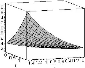
Figure 1. u(x,y,t) for = 0.8, y=0.1.
Figure 2. The comparison of u(x,y,t) for = 0.8, y=0.1 with the exact solution of u for y=0.1.
Figure 3. v(x,y,t) for = 0.8, y=0.1.
Figure 4. The comparison of v(x,y,t) for = 0.8, y=0.1 with the exact solution of v for y=0.1.
Figure 5. w (x,y,t) for = 0.8, y=0.1.
Figure 6. The comparison of w (x,y,t) for = 0.8, y=0.1 with the exact solution of w for y=0.1
FPDEs approximations solutions.
CONCLUSION
Three-dimensional differential transform have been applied to non-linear systems of FPDEs. The result for the example showed that exactly the same solutions have been obtained with homotopy analysis method. The present method reduces the computational difficulties of the other methods and all the calculations can be made simple manipulations. The results show that FPDTM is powerful mathematical tool for solving systems of nonlinear partial differential equations.
REFERENCES
Arikoglu A, Özkol I (2007). Solution of fractional differential equations by using differential transform method, Chaos Solitons Fractals pp. 1473-1481.
Caputo M (1967). Linear models of dissipation whose Q is almost frequency independent. Part II, J. Roy. Austral. Soc. 135: 29-539. Hang X, Shi-Jun L, Xiang-Cheng Y (2009). Analysis of nonlinear
fractional partial differential equations with the homotopy analysis method, Commun. Nonlinear Sci. Numer. Simulat. 14(4): 1152-1156. Hilfer R (Ed) (1999). Applications of fractional calculus in physics,
Academic press, Orlando.
Hosseini MM, Jafari M (2009). A note on the use of Adomian decomposition method for high-order and system of nonlinear differential equations, Commun. Nonlinear Sci. Numer. Simulat. 14(5): 1952-1957.
Jafari H, Seifi S (2009). Solving a systems of nonlinear fractional partial differential equations using homotopy analysis method, Commun. Nonlinear Sci. Numer. Simulat. 14: 1962-1969.
Jafari H, Seifi S (2009). Homotopy analysis method for solving linear and nonlinear fractional diffusion-wave equation, Commun. Nonlinear Sci. Numer. Simulat. 14(5): 2006-2012.
Lei W, Li-dan X, Jie-fang Z (2009). Adomian decomposition method for nonlinear differential-difference equations, Commun. Nonlinear Sci. Numer. Simulat. 14(1): 12-18.
Odibat Z, Momani S (2006). Application of variational iteration method to nonlinear differential equations of fractional order, Int. J. Nonlin. Sci. Numer. Simul. 7(1): 15-27.
Padovan J (1987). Computational algorithms for FE formulations involving fractional operators,Comput. Mech. 5: 271-287.
Podlubny I (1999). Fractional differential equations. An introduction to fractional derivatives, fractional differential equations, some methods of their solutionand some of their applications. SanDiego: Academic Press.
Zhou JK (1986). Differential transformation and its applications for electrical circuits, Huazhong university Pres, Wuhan,China.