İSTANBUL BİLGİ UNIVERSITY INSTITUTE OF GRADAUTE PROGRAMS ECONOMICS MASTER’S DEGREE PROGRAM
A SECTOR LEVEL ANALYSIS FOR MACROVARIABLES AND STOCK INDICES IN TURKEY
Gizem ÇETİN 117622001
Assoc. Prof. Serda Selin ÖZTÜRK İSTANBUL 2020
A SECTOR LEV ELANALYSIS OF MACROVARlBLES AND STOCK RETURN SIN TURKEY
MAKROGÖSTERGELER VE STOK GETİRİLERi İLİŞKİSİNİN SEKTÖR BAZINDA ANALİZi
T <-z Danışmanı:
Jüri Üy esi: Jüri Üy esi:
Gizem ÇETİN 117622001
Doç. Dr. S.:rda Selin ÖZTÜRK İstanbul Bilgi Oni,'Crsitesi
Dr. Öğr. Fatma Didin Sönmez İstanbu) Bilgi Üni,'Crsitesi Doç. Dr. Ender DEMİR İs"tanbul Modeniyct Üni,'Crsitı::si
Tezin Onaylandığı Tarih: 02.01.2020 Toplam Sayfa Sayısı: 89
Anahtar Kelimeler (fürkçc) Anahtar Kelimeler (İngilizce)
1)Sıok g<1irisi 1) Stock returns
2) Döviz Kuru 2)Exchange Rate
3) Faiz 3) lntcrcst Rate
4) Para Anı 4)Moncy Supply
iii
ACKNOWLEDGEMENT
First of all, I would like to express my gratitude and thanks to my advisor Assoc. Prof. Serda Selin Öztürk for her contributions and kindness, and of course helps during my study.
Also, I would like to thank my friends, Hasan Demirtaş, Deniz Benli and Mustafa Erdem for their supports at every stage of the process.
Moreover, I would like to thank Dr.Seçkin Özbilen for his support during the program.
Then, I would like to thank my uncle Assoc. Prof. Hüsamettin Çetin for his encouragement and guidance.
Last but not least, I would like thank my parents Dilek and Bahattin Çetin for standing by me every time.
Gizem Çetin İstanbul 2020
iv
TABLE OF CONTENTS
ACKNOWLEDGMENT...iii
ABBREVIATIONS……….… vi
LIST OF FIGURES……….………….…...vii
LIST OF TABLES ……….……... viii
ABSTRACT………..ix
ÖZET………...………...x
INTRODUCTION………...1
1.MACROVARIABLES AND STOCK RETURNS RELATIONSHIPS...2
1.1. Money Supply and Stock Returns...2
1.2. Inflation and Stock Returns...2
1.3. Interest Rate and Stock Returns...3
1.4. Exchange Rates and Stock Returns...3
1.5.Economic Activity and Stock Returns...4
1.6.Oil Prices and Stock Returns...4
1.7.Effects of Local versus Global Factors on Stock Returns...5
1.8. Financial Crisis of 2008 and Repercussion of Stock Markets…...6
2. A BRIEF ON ISTANBUL STOCK EXCHANGE...8
3.LITERATURE REVIEW……….11
4.DATA………...20
4.1.CHOICE OF VARIABLES………...20
v
5.METHODOLOGY………30
5.1.THE VAR METHODOLOGY………...30
5.2.TEST OF STATIONARITY………...32
5.3.DETERMINING LAG LENGTH………....36
5.4.TEST OF CO-INTEGRATION………...37
6.EMPIRICAL RESULTS………...41
6.1.VAR RESULTS: XU100………....44
6.2.VAR RESULTS: XUHIZ...46
6.3. VAR RESULTS: XUSIN………...47
6.4. VAR RESULTS: XUMAL………49
6.5. VAR RESULTS: XUTEK...51
CONCLUSION………53
REFERENCES………55
APPENDIX………...63
APPENDIX 1: AUGMENTED DICKEY FULLER TESTS, E-VIEWS……....63
APPENDIX 2: LAG LENGHT, SCHWARZ INFORMATION CRITERION (SIC), E-VIEWS………....74
APPENDIX 3: JOHANSEN CO-INTEGRATION TESTS, E-VIEWS……….76
APPENDIX 4: VAR RESULTS, E-VIEWS………...78
vi
ABBREVIATIONS ADF: Augmented Dickey Fuller
AIC: Akaike’s Information Criteria SIC : Schwarz Information Criteria GDP: Gross Domestic Product VAR: Vector Autoregressive
VECM: Vector Error Correction Model
GARCH: Generalized Autoregressive Conditional Heteroskedasticity NARDL: Non-linear Autoregressive Distributed Lag
APT: Asset Pricing Theory
CBRT: Central Bank of the Republic of Turkey FED: Federal Reserve Bank
PPI: Producer Price Index CPI: Consumer Price Index ISE: Istanbul Stock Exchange XUHIZ: Services Index XUMAL: Financial Index XUSIN: Industrial Index XUTEK: Technology Index
vii
LIST OF FIGURES
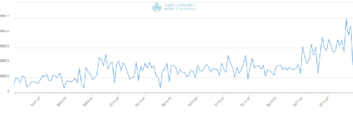
Figure 2.1. Total Trading Volume (Thousand TL)...8
Figure 2.2. Total Trading Volume...9
Figure 4.1.All BIST Indices from 2006 to 2018...21
Figure 4.2.XUHIZ Closing Price from 2006 to 2018...21
Figure 4.3: XUMAL Closing Price from 2006 to 2018...22
Figure 4.4: XUSIN Closing Price from 2006 to 2018 ...22
Figure 4.5: XUTEK Closing Price from 2006 to 2018………..………....23
Figure 4.6: USD/TRY Exchange rate from 2006 to 2018……….23
Figure 4.7: One-year deposit rate from 2006 to 2018...24
Figure 4.8: Consumer Price Index from 2006 to 2018...25
Figure 4.9: Industrial Production Index from 2006 to 2018...26
Figure 4.10: US Money Stock M2 (Billions of Dollars) from 2006 to 2018...26
Figure 4.11: 10-Year Treasury Constant Maturity Rate (%) from 2006 to 2018 ………...27
Figure 5.1: Econometric Research Methodology ………...30
Figure 5.2: All BIST Indices in Log level...35
viii
LIST OF TABLES
Table 4.1: Descriptive Statistics of Macrovariables...28
Table 4.2: Descriptive Statistics of BIST Indices at Log Level………...28
Table 4.3: Descriptive Statistics of BIST Indices at First Difference………..29
Table 5.1: Unit Root Test, Augmented Dickey-Fuller Test of BIST Indices..34
Table 5.2: Unit Root Test, Augmented Dickey-Fuller Test of Macrovariables...35
Table 5.3: Lag Length Test, Schwarz Information Criterion (SIC) ...37
Table 5.4: Johansen Cointegration Test: Trace Results...40
Table 5.5: Johansen Cointegration Test: Maximum Eigen Value Results...40
Table 6.1. Glossary of Variables……….42
Table 6.2: Model Statistical Test Results………...43
Table 6.3: VAR Results of XU100 for All Periods...…..44
Table 6.4: VAR Results of XUHIZ for All Periods...46
Table 6.5: VAR Results of XUMAL for All Periods...47
Table 6.6: VAR Results of XUSIN for All Periods...49
ix
ABSTRACT
The way of macroeconomical factors affect stock returns has been discussed for long time by investors. The paper aims to examine stock returns and macroeconomic variables relationship on sector level for Turkey by covering period of 2006:1 and 2018:12. The choosen domestic economical factors are exchange rate USD/TRY, consumer price index, industrial production and 1-year deposit rates ; international factors are US M2 money supply and 10-year treasury constant maturity rate. BIST00, service, industry, technology and financial sector indices are selected as endogenous variables in VAR model. The main findings are while exchange rate USD/TRY, 1-year deposit rate and US M2 money supply have negative effects on stock indexes; industrial production influence positively compatibly previous researhes. In addition, global factors found to be significant on returns like local factors. The test results also show that Turkish consumer price index and US long term treasury yield do not have any effect on chosen sector indices. Moreover, there is no bilateral correlation among BIST100 index and other sector indices between 2006-2018.
x
ÖZET
Makroekonomik göstergelerin stok getirilerini nasıl etkilediği uzun zamandır tartışılmaktadır. Bu çalışmanın amacı 2006-2018 yılları arasında BIST endeks getirileri ve makroekonomik değişkenler arasındaki ilişikiyi sektör bazında incelemektir. Tüketici fiyat endeksi, sanayi üretim endeksi, 1 yıllık mevduat faizi ve dolar kuru lokal faktörler olarak seçilirken, ABD M2 para arzı ve 10 yıllık hazine getiri oranları global faktörler olarak seçilmiştir. Vektör otoregresyon modelinde endojen değişkenler olarak BIST100 endeksi, servis, sanayi, finans ve teknoloji sektör endeksleri kullanılmıştır. Sonuçlarda, önceki araştırmalara uyumlu şekilde, dolar kuru, faiz oranları ve para arzı stok getirilerini negatif olarak etkilerken, sanayi üretim endeksi pozitif olarak etkilemektedir. Bunun yanında, global faktörlerinde getiri üzerinde lokal faktörler gibi etkili olduğu görülmüştür. Tüketici fiyat endeksi ve ABD hazine getiri oranlarının stok getirileri üzerinde etkisi olmadığı gözlemlenmiştir. Ayrıca 2006 ve 2018 yılları arasında BIST100 ve diğer sektör endeksleri arasında ikili bir ilişkiye rastlanmamıştır.
ANAHTAR KELİMELER: Stok getirisi, Döviz kuru, Faiz oranı, Para Arzı, BIST
1
INTRODUCTION
The relationship between macroeconomic factors and share prices has been deliberated both in economics and finance literature since the beginning of 1970. The anomalous findings and ever-growing ideas modernized this issue. Unanticipated share price volatility in world markets during 1980’s and 1990’s increased interest on this relationship. Some researchers stated that this volality was resulted by speculative movements, some others focused on causality among share returns and macrovariables.
The present value or discounted cash flow is the most commonly used model for share evaluation. In this model, share price evaluation is directly related with the discount rates and dividends which are affected by real economic activity and government economic decision immediately. Therefore, origin of the debate about the relationship between share prices and macroeconomic indicators stemmed from this vital connection. Flannery and Protopapadakis (2002) claimed that macroeconomic variables affected the discount rate based in discounted cash flow model and so firms’ impetus to generate cash flow. By considering macrovariables effects on income and cost structure of the firms, stock returns movements can be foreseen.
This thesis tries to explain the relation between macrovariables and stock returns. Although there are wide range research even for stock returns of emerging markets, due to limited research in sector level analysis on stock returns for Istanbul Stock Exchange, this subject is valuable for Turkey case and will be elaborated in this paper.
This study consists of six parts. Part 3 reviews previous literature associated with the subject. Part 4 describes the data set and examines first set of results, and in section 5 the statistical methodology which is covered in the analysis is illustrated. The empirical findings are detailed in Section 6. Eventually, conclusion section presents the results and evaluations as a whole.
2
1.MACROVARIABLES AND STOCK RETURNS RELATIONSHIPS 1.1.Money Supply and Stock Returns
The very first study about relationship between money supply and share prices was prepared by Palmer (1970). The research showed that change in money supply influenced the share prices. Many researcher supported this statement; as Ho (1983) found that money supply change caused changes in stock prices unambiguously for Hong Kong and Japan; and then Thornton (1993) concluded that there were feedback effects between money supply and stock prices. The common accepted wisdom tells changes in money supply affect the financial market by impacting on general economy immediately. Loanable funds’s amount in the market is directly affected by interest rate through money supply adjustment. When money supply rises, interest rates fall due to increase in the amount of loanable fund. On the contrary, Durham (2003) stated that monetary policy did not demonsrate any relation between easing or tightening money supply cycles and stock prices, in other words the correlation between money supply and stock returns was weak or nonexistent.
1.2.Inflation and Stock Returns
The protection against inflation is very important for investors who have the expectation that revenue genereated from asset acquisition should be a hedge agaist inflation loss in the light of Fisher hypothesis. A reverse relation among stock prices and inflation level was presented by first Fama (1981) and later supported by Lee (1992). In detail, mentioned correlation was not a casual relation but was a proxy for a positive correlation among stock prices and real activity, plus was induced by a negative correlation between real activity and inflation. From a different point of view, the negative correlation results from investors preference changing from stocks to interest bearing assests during high inflation periods. On the contrary to these negative relationship claims, Kessel (1956) stated that if a firm is a net debtor, an increase in unanticipated inflation will rise the firm’s value depending on
debtor-3
creditor hypothesis. Kessel was also supported by Abdullah’s (1993) Granger causality test which revealed positive relation among price level and stock prices. 1.3.Interest Rates and Stock Returns
Researches so far show that there is a strong relationship between interest rates and share prices. Change in interest rates affects borrowing cost and profitability of a company. In this sense, a decrease in interest rates lowers the cost of borrowing thus incentivize the firm for expansion which may lead an increase future expected value of a firm. Besides a direct effect on share values, interest rate affects returns of alternative investment tool like bonds. Thus it leads change in stock demand in the market. Cook and Hahn (1988) found that when interest rate increased, stock market exhibited a downward trend as a short term reaction (announcement effect), if interest rate increased vice versa. Saunders and Yourougou (1990) examined the side of firm’s assets and liabilities and interest sensivity relations and found that industrial firms were less fragile to fluctuations in nominal interest rates than securities claim on monetary assets.
1.4.Exchange Rates and Stock Returns
The currency value fluctuations affects corporate earnings therefore the exchange rate has been scrutinized to explain stock returns for many years. Although there is no satisfactory findings about stock price reaction to exchange rate volatillity in early research because of fix regime of Bretton Wodds, the impressive growths in the world trade and capital movements have done exchange rate as more important topic recently. The possible explanations for stock price and exchange relations: change in exchange rate, first of all, influence value of firm’s portfolios. Second, being importer or exporter is matter. If country the country is an exporter one, currency depreciation may increase its competitiveness and positively influences stock price. Third, rather than a casual correlation between stok prices and exchange rates, there may be indirect relation because of the links betweeen exchange rate & economic activity and economic activity & stock price. Solnik (1987) found a positive correlation amoung share returns and foreign exchange rate. Aggarwal
4
(1981) claimed that this relationship was stronger than in the short term compared to long term. On the contrary, Soenen and Hennigar (1988) concluded in statistically meaningful reverse effect on share returns of exchange rates. Rittenberg (1993) analyzed the issue for Turkey by Granger causality test, he found a casuality driving from equity price level to exchange rate but there existed no feedback causativeness from exchange rate changes to price changes. Anlas (2012) examined the impacts of foreign exchange rates changes on ISE, from January 1999 to November 2011. By applying the techniques of time series analysis he concluded that the changes in domestic U.S. Dollar and Canadian dollar were positively related to changes in ISE 100.
1.5.Economic Activity and Stock Returns
The findings of previous studies about correlation between economic activities and stock returns are contradictory. Abdullah and Hayworth (1993) claimed that economic actions influenced share prices because of their effects on firm incomes.The general opinion regarding this relation is increasing economic activity leads a positive impact on stock returns. Mahdavi and Sohrabian (1991) looked from different point of views and stated that annual stock returns succesfully predicted growth slowdowns or recessions, in other words; GNP follows the trend of share prices. The idea is investestment decision mirrors investors expectation about stock prices thereby future firm profits. Thus level of aggregate domestic and real economic action may be estimated from stock market activity. Kwon and Shin (1999), Nasseh and Strauss (2000) and Binswanger (2004) used industrial production index as a proxy for economic activities. Industrial production index is also used in this paper due to the lack of monthly GDP data.
The correlation among trade balance and stock returns has not been studied much in the literature. However, it is taken into consideration in few article due to growing open economy concept and its implicit relations with other variables, specially exchange rates.Fifield et al. (2002) and Acikalin et al. (2008) analyzed the effect of current account balance and foreign trade balance in their studies and could not find any significant relationship.
5
1.6.Oil Prices and Stock Returns
Oil prices influences production costs and inflation rates. Hence these prices has direct impact both on stock market returns and real economic activity. The 1973 oil price shock and the subsequent recession led to many studies analyzing the interrelation among economic variables and oil price changes. General opinion about this relationship is that oil prices exercise an adverse influence in stock markets. Filis at all (2011) contributed the topic with the findings that oil prices behaves parallel with stock markets during 2008 global financial crisis. Therefore in the periods of economical turmoil, the oil is an unsecure investment option for hedge against stock market losses. Basher at all (2012) investigated oil price, exchange rates and emerging stock market relations.The findings revealed a positive shocks to oil prices tend to reduce emerging market stock prices and US dollar exchange rates in the short term. The model also emphasized stylized facts concerning movements in oil prices. A positive oil production shock decreased oil prices while a positive shock to real economic activity rose oil prices. Another evidence indicated that increasing emerging market stock prices rose oil prices. 1.7. Effects of Local versus Global Factors on Stock Returns
Previous literature on the subject is mainly concentrated on developed markets. However, a enormous amount of capitals currently moves into emerging stock markets with the aim of efficient asset allocation and enlarged liquidity in these markets thanks to the positive effects of liberalizations. This makes it interesting to explore likely correlations among emerging stock markets and country-specific macroeconomic factors. In this aspect, it has been discussed that local variables rather than global ones are the main source of equity return variation in these markets. Bilson et all (2001) stated that integration level influenced the priority of international versus domestic factors. If we accept that the markets are not perfectly integrated, especially in scope of emerging markets, then it is likely that national factors may be more relevant than global ones. Similarly, Karolyi and Stulz (2003) investigated the international finance literature in order to evaluate impact of international factors on financial asset demands and prices. The results indicated
6
that risk premium of a country and exchange rate risks affect expected returns. In addition to this, anticipating the extent to which home bias affects the asset prices gave idea regarding size of local influences. Moreover, equity flows and cross-country correlations are the signals of global influences on asset prices. Durand at all (2006) searched ‘home grown’ factors’ effects for Australian equity returns by using Fama-French three factor model and found that largest firm in the Australian market was simply part of the larger US market, on the contrary small firm were affected local factors. Cauchie at all (2004) focused on Swiss stock market and concluded that both global and local economic conditions affected stock returns. In the scope of international market integration, Beckers at all (1996) compared national versus global influences on equity returns and found that international effects and countrywide effects had roughly equal status in explanation the common movements in share returns. It was shown that there was a tendency to high integration within European Union, but not universal. Rizwan and Khan (2007) studied stock returns and country and global factors relation in an emerging market Pakistan using VAR model. The results showed that both country and global factors were significant.
1.8. Global Financial Crisis of 2008 and Repercussion of Stock Markets Since sample over 2006-2018 covers global financial crisis of 2008, effects of crisis on stock returns in different markets should be examined. Luchtenberg and Viet (2015) studied global contagion and its causes in time of 2008 financial crisis. It was concluded that contrary to earlier crises contagion subsequent the 2008 global financial crisis was not limited to emerging markets. The United States and other developed financial markets in the sample conveyed and received contagion. In addition, variables were compared as before crisis and during the crises separetely. Interest rate, inflation rate and industrial production contributed to international contagion. Didier at all (2011) stated that countries with fragile banking and corporate sectors showed high percent comovement with US market by analysing period previous and following the bankrupt of Lehman Brothers. This finding showed that comovement was mainly stemmed from financial connections.
7
Similarly, Bekaert at all (2014) claimed that contagion from the United States was small amount, on the contrary there were considerable contagion from local markets to individual local portfolio, with its pressure that situation gives inversely associated with the economic fundamentals’ solidness of a country. This conforms the “wake‐up call” hypothesis, with markets focusing more on country‐specific characteristics during the crisis. Nikkinen at all (2012) investigated effects of 2008-2009 crisis on Baltic region, countries namely Estonia, Latvia and Lithuania. Previous researches revealed that while mature stock markets were vastly integrated, emerging markets might be segmented. The way this integragration changes in crisis is questioned. The findings indicated that the Baltic stock market were apperantly segmented previously the crisis and they were highly integrated through the crisis. Frankel and Saravelos (2010) investigated leading indicators of financial crisis. For the 2008-09 crisis, they used six different variables to measure crisis incidence: fall of GDP and industrial production, currency depreciation, stock market performance, reserve losses, or participation in an IMF program. The results showed that level of reserves in 2007 appeared as a statistically significant leading indicator of the crisis. In addition to reserves, real appreciation was a statistically significant predictor of devaluation and a measure of exchange market pressure during the crisis.
8
2. A BRIEF ON ISTANBUL STOCK EXCHANGE
Before 1980, government activities and restrictions ruled Turkish economy. There was no capital market and foreign exchange operations were prohibited in the sense of centralized and state-oriented economy. The early time of 1980s witnessed a remarkable development in the Turkish capital markets, associated with both the legislative framework and the institutions to reach highly liberalized and globally integrated economy. IMF-supported stabilization program had executed in 1980. After thus Turkish economy politics transformed from an inward-oriented strategy to an outward-oriented one.In 1981, the "Capital Market Law" was legalized. The principles regarding operational procedures were agreed in the congress and Istanbul Stock Exchange was officially initiated at the end of 1985. Istanbul Stock Exchange (ISE) as an self-governing, professional organization in the beginning 1986 was started trading with 42 companies. ISE filled a gap as an only establishment for securities exchange in Turkey. This corporation enabled trading in equities, bonds and bills, revenue-sharing certificates, private sector bonds, foreign securities and real estate certificates likewise international securities.
2.1. Total Trading Volume (Thousand TL)
9
Figure 2.2.Total Trading Volume ( Thousand)
Source: CBRT
Since 1994 Turkish stocks in the market rose more than 250 times by 1997. Daily trading volume passed over $150 million. In trading volume, ISE was the eighth largest of the twenty-two European stock exchanges by outdistancing Madrid, Copenhagen, Oslo, Brussels and Vienna.Recently, the number of listed companies has reached 489 with market capitalization of $163 billion and the daily trading volume 2 billion.
As it seen figure in 2.1 and 2.2 which shows trading volumes from 2006 to 2018, after 2018, in both figures, a sharp decrease is observed with effect of 2018 ongoing crisis. Another slump in stock performance experienced in gobal financial crisis of 2008. In 2008, substantial falls experienced in world stock markets. The global economic crisis also influenced Turkish economic system. Accordingly the falls of stock markets in worldwide, a significant decrease also observed in ISE. In 31.12.2007, the index was 55.538 point. This score declined 51,62% in 31.12.2008 and reached 26.864 point. Downward trend that occured in ISE had maintained in 2009 and index declined to the point of 23.055 on march 2009.
The comprehensive transformation in Turkish economy was required Foreign Policy Investment (FPI) and Foreign Direct Investment (FDI) measures that regulates foreign investors activities in 1980 and 1989. An empirical result revealed that shares owned by foreigners on the Istanbul Stock Exchange (ISE) had been increasing since 1995 and its was about 50% in 2003. (Gazioglu, 2003). Today, foreign investor share in stock trading is approximately 65%. Akar (2008) stated
10
that there is a dynamic connection between ISE stock price and net foreign trading volume. In addition, the causality running from index price to net foreign trading volume is statistically more powerful.
From market efficiency perspective, previous studies showed that BIST follows random walk hypothesis but exhibits weak form efficiency. (Gozbası, Kucukkaplan and Nazlıoglu, 2014).
Hence, it may be concluded that former price information was reflected on market prices and prices moved independently from each other. In this sense, it is impossible for a trader who benefits from technical analyses by looking former price information to gain more profit than the one who does not have this information and to get above average. (Kılıc and Bugan, 2016)
11
3.LITERATURE REVIEW
The relationship between macroeconomic factors and change in stock prices has been the subject of many researches so far. In this section, the studies that investigate this relation will be reviewed. Although this relationship has been discussed intensively in many international markets, Turkey scope has been made less interference to evaluate.
One of the early research, Ratanapakorn and Sharma (2007) scrutinized long run and short run relationships among stock index (S&P 500) and six macroeconomic factors over the term 1975:1–1999:4. The Granger causality was utilized and it was found that while stock prices exhibited a reverse relation with long-term interest rate, there were positive impact of money supply, industrial production, inflation, the exchange rate and the short-term interest rate on stock prices.
Humpe and Macmillan (2009) studied the way of macroeconomic variables affect stock prices in the US and Japan. A cointegration analysis was used to figure out the long run relationship between industrial production, the consumer price index, money supply, long-term interest rates and stock prices in the US and Japan. According to results, stock prices were positively correlated with industrial production but negatively correlated with both the consumer price index and the long-term interest rate. Moreover, a trivial (but positive) affiliation between the US stock prices and the money supply was resulted. What’s more, two cointegrating vectors for the Japanese data was detected where one vector implied a positive relation with industrial production and a reverse relation with money supply. Another cointegrating vector demonstrated that industrial production negatively affected by the consumer price index and a long-term interest rate. These conflicting consequences may be due to the crash in the Japanese economy in the 90s and results of liquidity trap.
Gjerde and Sattem (1999) examined whether relationship between stock returns and macroeconomic variables from major markets are valid in a small, open economy by utilizing the multivariate vector autoregressive (VAR) approach on Norway. It
12
was concluded that coherently with US and Japanese outcomes, real interest rate affected both stock returns and inflation, and the stock market responded accurately to oil price changes. Besides, the stock market displayed a delayed reply to variations in inland real activity.
Asprem (1989) studied on similiar topic for other European countries and explored the connections among stock indices, asset portfolios and macroeconomic factors in selected countries. It was shown that employment, imports, inflation and interest rates were reversely related to stock prices. The relations among stock prices and macroeconomic factors were shown to be the strongest in Germany, the Netherlands, Switzerland and the United Kingdom. An intense correspondence was observed among the above mentioned countries except UK.
Moving to another part of Europe, Samitas and Kenourgios (2007) studied the extent to which current and future domestic and international macroeconomic factors could enlighten long and short term stock returns in east European countries namely Poland, Czech Republic, Slovakia and Hungary. Leading western European countries were included in the empirical analysis, while US was taken as a "foreign global influence”. Utilizing the present value model of stock prices including cointegration and causality tests, it was found that stock markets in eastern European were partly integrated with foreign financial markets, while inland economic activity and the leading European countries were more prominent factors on these stock markets than the US global factor.
Another study related to European countries where Papapetrou and Hondroyiannis (2001) analyzed the bilateral relation between indicators of economic activity. How economic activity affected the performance of the stock market in Greece was searched. An empirical finding showed that stock returns did not cause any change in real economic activity but the macroeconomic activity and foreign stock market changes elucidated partly stock market movements. Oil price changes explained stock price movements and had a reverse impact on macroeconomic activity. Similarly in US, Serfling and Milijkovic (2011) analyzed the relation between dividend yield on the S&P 500 Index, 10 year treasury yield, share price level of
13
S&P 500 Index, money supply, industrial production and consumer price index (CPI) in the period of January 1959 to December 2009. Vector Error Correction Model (VECM) was employed to examine the possible simultaneous and cross short term relations between the variables and reached that there existed important interactions without lag. Specifically, endogeneity among the the selected factors in a model could be observed to some extent most of the time. One of the main consequence of this study that taking into account only a direct cause and effect relationship between these factors would be inadequate so endogeneity of macroeconomic and firm-specific factors was required to be considered by investors during prediction of econometric models.
Chung and Tai (1999) inspected relation between current economic activities in Korea and stock market returns by utilizing a cointegration test and a Granger causality test. As a result of regression; it was suggested that stock price indices exhibited a cointegration relation with the macroeconomic variables namely, production index, exchange rate, trade balance, and money supply that provides a direct long-run equilibrium relation with each stock price index, i.e. implied long run equilibrium among the variables of interest.
Besides developed countries, there are some articles about developing countries regarding macroeconomic variables and stock returns relations even if they attracted far less attention than the developed ones.
Sing, Mehta and Varsha (2010) studied the casual relation among index returns and certain key macroeconomic factors for Taiwan. The findings revealed that gross domestic product (GDP) influenced returns of all portfolios. In addition, inflation, exchange rate, and money supply inversely affected returns of portfolios in big and medium firms.
Regarding to Latin American markets, Abugri and Benjamin (2008) analyzed a very similar topic; practical relation between macroeconomic volatility and stock prices by using VAR model. The chosen variables were key macroeconomic indicators such as exchange rates, interest rates, industrial production and money
14
supply. An emperical evidence showed that the international factors were important in elucidation returns in all markets constantly.
There are several studies that search macroeconomic varibles and stock return causality on Turkey specific. In one of these studies, Erdem & Arslan (2005) searched about volatility of ISE indexes with monthly data from January 1991 to January 2004, using explanatory indicators: exchange rate, interest rate, inflation, industrial production and M1 money supply. The Exponential Generalized Autoregressive Conditional Heteroscedasticity model was employed to check univariate volatility spillovers for macroeconomic factors. According to results, a solid volatility spillover running from inflation and interest rate to stock price indexes were observed in one direction. There were spillovers driving from M1 money supply to financial sector index, and from exchange rate to both ISE 100 and industrial sector index. There existed no volatility spillover from industrial production to any indices.
Having looked at recent studies, Tiryaki, Ceylan & Erdoğan (2018) examined the impacts of industrial production, money supply and real exchange rate on stock returns in Turkey utilizing the non-linear autoregressive distributed lag (NARDL) model over two different time span; 1994:01–2017:05 and 2002:01–2017:05. It was found that the effects of the changes in chosen variables on stock returns were asymmetric, and the asymmetries were bigger after the 2002 sub-period in comparison with the full sample period. The findings suggested that tight monetary policies seemed to impede the stock earnings more than easy monetary policies that stimulate them.
Dayıoğlu & Aydın (2019) also examined the relationship between BIST-100 Index and a set of macroeconomic variables volatility using VAR model. The study found that exchange rate and industrial production had an important influence on stock market volatility.
Demirtaş, Atılgan & Erdoğan (2015) employed an APT model to investigate equity return exposure to various macroeconomic factors. According to findings, there was
15
important reverse relationship among interest rate betas and future equity returns. Karakuş and Bozkurt (2017) studied effects of financial indicators and macroeconomic variables on firm value. To that end, firm’s quoted in BIST-100 panel data analysis was implemented. It was concluded that there existed reverse relation among debt ratio and stock returns. Otherwise, return on assets and net working capital turnover had a positive effect on stock returns. By considering macroeconomic variables, a inverse correlation among consumer price index and stock returns was identified. Beside, unemployment, gross domestic product, and exchange rates positively influenced stock returns.
Using a multivariate approach, Muradoglu, Taskin and Bigan (2000) analyzed the correlation among stock returns and macrovariables for emerging markets, inclusive of Turkey. For each country, Granger casuality test was employed and it was shown that local factors were important in determining stock returns. The results further suggested that bivariate causality among macroeconomic variables and stock returns occurred with the size of the stock markets, and their integration with the world markets.
Moreover, direction of the relation from macroeconomic factors to stock returns is assumed to be unidirectional. However, it is not the case. Harvey and Bekaert (1998) stated that dynamic links between macrovariables and stock returns in emerging countries had been ignored mainly due to overwhelming infleunce of governments in economic activity and low volume of trade in the markets. Nowadays, with the effects of liberalization and globalization, there are many researches about stock price effects on macrovariables. Gençtürk at all (2011) investigated casual relationship between BIST stock price, USD/TRY exchange rate, consumer price index, interest rates and industrial production employing VECM. It is concluded that the presence of long term relation was solely among BIST stock price and industrial production. A one directional casuality running from stock price to industrial production was found. Buyuksalvarcı and Abdioglu (2010) examined correlations between stock price and macro variables specifically foreign exchange rate, gold price, broad money supply, industrial production index
16
and consumer price index in Turkey. The results showed that there was a one directional long term correlation from stock price the macrovariables. Hence the stock market might be counted as an prominent indicator future growth. Nazlioglu at all (2010) examined the short and long term correlations among stock market performance and economic growth for emerging countries, including Turkey. The findings demonstrated that stock market was an stimulus for economic growth in the short term. In addition to this, the relation among stock market performance and economic growth was varying with the size of stock market. The performed analysis suggested that in markets with comperatively small national market capitalisation like Turkey, causality derived from stock market to economic growth. However, there did not exist such causal link for Brazil and India which have relatively larger market cap. Thus it is concluded that the small stock market performance may be regarded as one of the leading factors of economic growth in these countries. Husain (2006) analyzed the causal relation between key indicators of the real sector of Pakistan economy and stock prices. The results demonstrated the existence of a long term relation among stock prices and the real sector variables. Considering the dynamic links, the findings suggested a unidirectional relation run from the real sector activity to stock market. That is to say, the stock market of Pakistan was not that developed to influence the real sector of the economy. Therefore, the market could not be regarded as the significant sign of the economic activity in Pakistan. Liu and Sinclair (2008) searched link among stock market performance and economic growth in Greater China: mainland China, Hong Kong and Taiwan utilizing a VECM. According to results, unidirectional causality driving from economic growth to stock price in the long term plus from stock price to economic growth in the short term. The results revealed that stock markets perform as a predictor of future economic growth. Filler at all (2000) answered the question of whether financial development causes economic growth or whether it is a consequence of rising economic activity by using Granger causality test. They concluded that stock market development led in currency value of a country. Bakarat at all (2016) examined another two developing market; Egypt and Tunisia in the scope of same subject. The results indicated that the stock market index in
17
Egypt might be clarified variatios in the CPI, exchange rate and money supply. Whilst stock market index in Tunisia was found to be as an explatanory factor for changes in interest rate. By supporting Harvey and Baekart, Carp (2012) stated that market capitalization and value of trading volume did not have any effect on growth, recalling inadequate stock market development in Romania resulted from weak regulation and insufficient transperancy.
The papers related to 2008 crisis effects on emerging stock market should be searched since the time span of interest covers global subprime crises in 2008. Jin and An (2016) investigated global crisis and developing stock market contagion for BRICS (Brazil, Russia, India, China and South Africa) countries. It was examined that the way of the BRICS’ stock markets affected in the context of 2007-2009 global financial crises by employing volatility impulse response. The results revealed that degree of stock market responses to such shocks varies from one market to another, based on the level of integration with the international economy. The stock market highly integrated with the U.S faced with adverse effects.
Segot and Lucey (2009) examined MENA countries in terms of the vulnerability to external financial crises. It was searched about contagion shift to the MENA region for a number of different crises episodes including 2007-2009 financial crisis. According to results, Turkey, Israel and Jordan were the most weak markets in crisis during the period of 1997-2009. The results suggested that MENA basis diversification strategies might be relatively insufficient during period of global turmoil. In addition to this financial perspective, the findings indicated that stock market development brought likely destabilization cost from an economic point of view. Maghyereh at all (2015) examined also MENA countries in the context of dynamic transmissions with US before and after crisis period. According to one evidence of this study, pre crisis relationship between US and MENA stock markets were weak and negligible. The regional comovement and volatility jumped during and after financial crisis. Moreover the effects of U.S. started to revert back and reached initial low level. Thus, it could be interpreted that the Middle East and North African shares were significant diversifiers for investors; specially in the long
18
term. Kassim (2013) studied the effect of the 2007 global crisis on the Islamic stock markets. These stock markets were analyzed for pre crisis 2005-2007 and crisis 2007-2010 period by employing ARDL approach and VECM. The results suggested that 2007-2008 global financial crisis led change in pattern of cointegration level of stocks markets. According to results, the Islamic stock markets did not reveal proof of a long-term equilibrium relation before the crisis but suggest otherwise in the crisis period. This emperical evidence supported time-varying aspect of stock market integration, as proposed by Bekaert and Harvey (1995). Therefore, there were potential diversification oppurtunities between the Islamic stock markets in the non-crisis period, and these diversification oppurtunities weaken in the crisis time. Another study, Mollah at all (2006) examined market integration among the US and other stock market during 2003-2013. It was suggested contagion in developed and developing markets in the both global and Eurozone crises time. The findings further suggested that contagion extent from the US to the other markets in crises period. The spread of bank risk among the US and other countries is the key transfer channel for inter-country relations.
Influences of 2008 crisis on Turkish stock market are widely discussed in the literature. Sekmen and Hatipoglu (2015) investigated the price and volatility behaviours of BIST against subprime crisis with daily data from June 2004 to June 2014. They employed GARCH and EGARCH model to detect volatility in three sub-terms; pre-crisis 2004-2007, crisis 2007-2009 and post crisis 2009-2014. It was found that subprime crisis caused an increase volatility in Turkish Stock Exchange. In addition, the results suggested leverage effects on the volatility of stock returns for full sample was observed and the crisis induced a noteworthy surge in the asymmetric parameter, which revealed that negative announcuments provoked higher effects on future volatility compared to positive ones. Çağıl and Okur (2010) studied effects of 2008 crises on Istanbul Stock Exchange employing a GARCH model for the period of 2004-2010. BIST100 and BIST30 indices were examined with daily returns data. They divided total sample two periods; before the bankruptcy 03-2008/09-2008 and after bankruptcy 09-2008/04.2009. The results
19
indicated that variance values were exhibited a substantial increase in the period of 2007-2010. In addition to this, resistance of volatility shock increased notably in this period. Celikkol at all (2010) analyzed the effects of Lehman Brothers collapse on the volatility structure on BIST-100 stock index by using ARCH-GARCH models. The results suggested that crisis peaked in Turkish stock market and volatility were higher in the bankruptcy annocument period. They also observed that standart deviation indeed volatility of BIST-100 rised for the period of crash. Average returns of the investors also inreased in paralell to higher risk in crisis period.
20
4.DATA
The hypothesis of this thesis is to demonstrate the relation among the macro indicators and stock returns on sector level for Turkish stock market, modelling the data by using the VAR. The period of interest is between 2006 and 2018. Four domestic and two global variables in the model were carefully selected by searching the relevant literature; consumer price index, exchange rate USD/TL, one year deposit rates-TL, production index as local factors and M2 US money supply and US 10 years treasury yield rate as global factors.
The sector stock indices are namely; services index XUHIZ, financial index XUMAL, industrial index XUSIN and technology index XUTEK. This section contains information about the variables used in the study.
4.1.CHOICE OF VARIABLES
The data of this study were taken from CBRT and FED as monthly-basis. The data includes the stock market values of the BIST 100 and the other sector indices quoted in BIST and selected macrovariables. The sample period covers 144 months during the period 2006 – 2018.
Figure 4.1 shows chosen sector indices’ performances between 2006 and 2018. All indices exhibit an upward trend during this period. Although XUMAL is best performer throughout the years, XUTEK has exceled in recent years. In addition, all indices has been affected by 2008 financial crises negatively. Investors’s portfolio experinced approximately 50% value lost. By taken consideration Turkish stock market in terms of foreigners’ transaction share, the level was more than half, about 66,5% as of November 2009. Therefore, the effects of the crisis deepened with the foreign funds outflows from the country in crisis. Recovery of the crisis had maintained until end of the 2010. Since, after Turkish constitutional referendum in september 2010 less volatile and more stable trend has been observed, stock indices are examined dividing the term 2006-2009 and 2010-2018. Moreover, if macro indicators are examined, it is seen that there are different patterns in
21
behaviour of variables in two periods especially, one year deposit rate, consumer price index, industrial production index and 10 year treasury constant maturity rate.
Figure 4.1. All BIST Indices from 2006 to 2018
XU100 XUTEK XUHIZ XUMAL XUSIN
Source: CBRT
As it is seen on the graph, figure 4.2 demonstrates services index price development in years. Currently, XUHIZ shows performance of 67 companies that serves in energy, transportation, retail, real estate, ready-made clothing sector. This index has employed by BIST since 1996.
Figure 4.2. XUHIZ Closing Price from 2006 to 2018
Source: CBRT
In figure 4.3, financial services index price development is demonstrated. XUMAL shows performance of 106 companies such as real estate investment, insurance
22
and pension companies, banks and investment conglomerates. This index has used by BIST since 1990 and it is the most damaged index in 2008 financial crises.
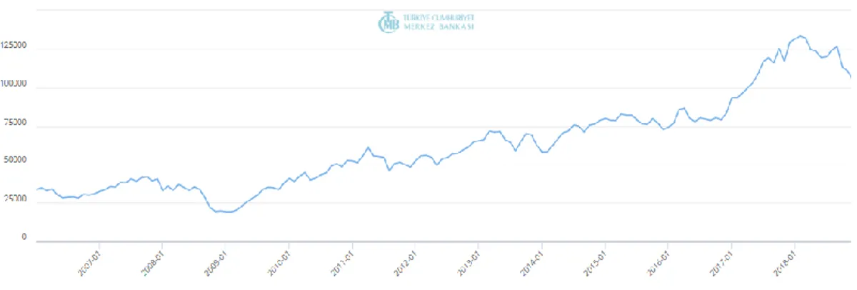
Figure 4.3. XUMAL Closing Price from 2006 to 2018
Source: CBRT
XUSIN represents stock performance of industiral companies quoted in BIST. This indicator includes 169 production company from different sector such as petrochemical, cement, automotive, food, textile industry. This index was integrated to BIST in 1990.
Figure 4.4. XUSIN Closing Price from 2006 to 2018
Source: CBRT
XUTEK denotes stock performance of technology companies quoted in BIST. This index has used since 2000 and represent 17 companies from telecommunication, software and information sector. By differentiating from other indexes, it shown poor performance until 2016 and has exhibited a rapid increase last 2 years.
23
Figure 4.5. XUTEK Closing Price from 2006 to 2018
Source: CBRT
The macrovariables which are taken from CBRT are one-year deposit rate, USD/TRY exchange rate, CPI (as a proxy for inflation) and industral production. Until 2014, f/x rate moved steadily, after then it has showed an upward trend. Exchange rates has slumped in 2018 with devaluation and TRY lost value approximately %40. The external shock caused by negative capital movements first hit the exchange rates in 2018. Ongoing currency crisis in 2018 may be reason of decrease in the BIST stock indices. As it seen on the graph, 2008 crises hardly affected exchange rate negatively.
Figure 4.6. USD/TRY Exchange Rate from 2006 to 2018
24
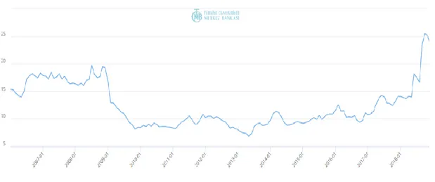
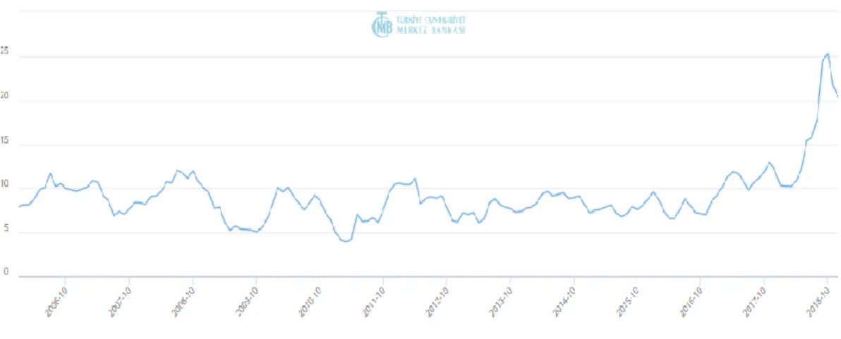
When the changes in interest rates are examined during the sample period, two striking trends are observed. The first is the downward trend that started in 2009 and the upward trend in 2018. As it seen in the figure 7, deposit rates follow different paths in periods 2006-2009 and 2010-2018. Increasing trend of interest rates in 2018 first reached the level before 2009 and even exceed this level later. 1-year deposit rate which was 20% on January 2009, decreased by 50% in one 1-year and was realized as 10%. Interest rates fell as the effects of the 2008 crisis waned and economic recovery started. In the second half of year 2018, it was increased by 10% compared and realized as 25%. It can be explained by the capital outflows from emerging market countries, which is true to Turkey, as well.
Figure 4.7. One-year Deposit Rate from 2006 to 2018
Source: CBRT
The relation among price level changes and stock prices are represented by changes in consumer price index in the study. Since CPI reflects the price of goods and services merchandised between the companies thus it affects the income of the companies. Moreover, CPI displays price movements that gives sign about supply and demand in the real economy. Although a fluctuating movement is observed before 2009, there is a more stable trend from 2010 utill 2018 in figure 8. From 2006 to 2018, an upward trend is observed which is very similar with M3 money supply in Turkey. In order to prevent endogenity between variables, cpi is choosen as an indicator.
25
Figure 4.8 Consumer Price Index from 2006 to 2018
Source: CBRT
The industrial sector is a component of GDP and one of the most significant drivers of domestic income and economic growth. The industrial sector, which makes a significant contribution to employment, also gives a significant impetus to growth. Therefore, industry production index acts as a proxy of gdp since it is mostly preferred as an indicator for growth data. Since the industrial production index is announced monthly, IP index is preferred rather than GDP in this study. Financial depression in 2018 also affected on industrial production in Turkey and its effects began in the last months of 2008. Industrial production started to diminish in August. This downward trend continued until March 2009. The contraction in industrial production index was 23.5 % in this term. In third quarter of 2017, with the effect high GDP growth rate, a sharp rise realized in industrial production. In 2018, a fall has started the because of ongoing crisis.
26
Figure 4.9. Industrial Production Index from 2006 to 2018
Source: CBRT
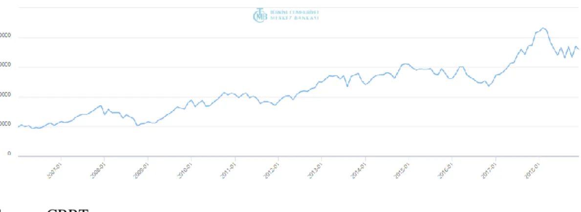
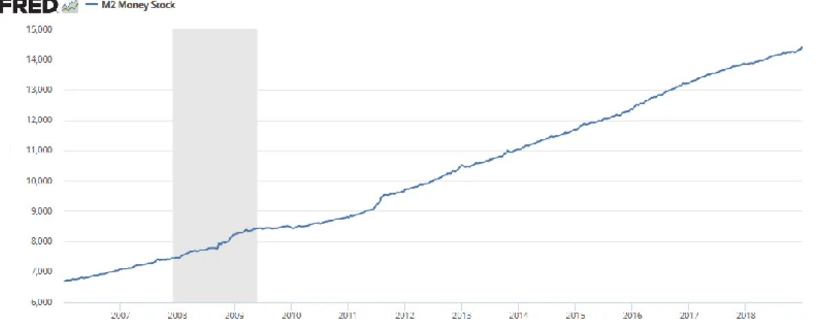
Apart from local macrovariables, two more indicators are selected globally: US money supply and 10-year treasury constant maturity rate. In general, if money supply increase, interest rate will decrease or vice versa. Central bank controls money in circulation by adjusting the interest rates. Main aim of the interference to money supply is to protect general price level. Money supply, which can also be defined as total purchasing power; important as a provider of investment, production and commercial activities. M2 consists of set of financial assets held principally by households. M2 consists of M1 plus: (1) savings deposits; (2) small-denomination time; and (3) balances in retail money market mutual funds. US money supply exhibits an gradually increasing trend throughout the years.
Figure 4.10. US Money Stock M2 (Billions of Dollars) from 2006 to 2018
27
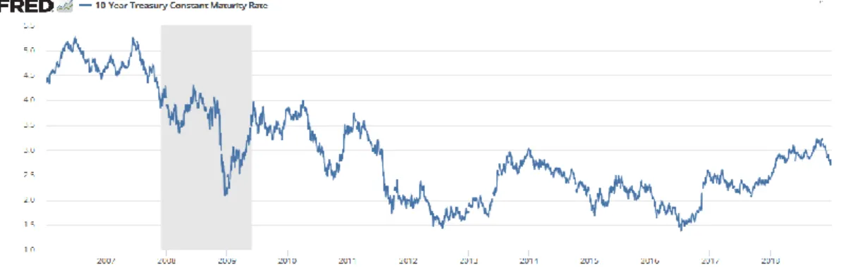
Federal Reserve Board publishes 10-year treasury constant maturity rate as an index depending on the average yield of a set of treasury securities after adjustment accordingly equivalent of ten years maturity. Yields on treasury securities at fix term are decided by the U.S. Treasury from the daily yield curve. That is based on the closing market-bid yields on actively traded treasury securities in the over-the-counter market. Government bonds maturing in ten years refer to long term interest rate which is one of the determining factor of business investment. While low long-term interest rate incentivizes new investments and high interest rates deters new investment decisions. US interest rates decreased after 2008 crises sharply in the scope of contractionary monetary policy that is seen in the figure 4.11.
Figure 4.11. 10-Year Treasury Constant Maturity Rate (%) from 2006 to 2018
Source: Federal Reserve Bank of St.Louis
4.2.DESCRIPTIVE STATISTICS
The descriptive analysis delivers a primary depiction of nature and volatility of the variables. Simultaneously, it compares the basic performance indicators of the variables, enabling an description about the way of interdependence among factors varies. Descriptive statistics will be useful to analysis the variables further. The mean, median, max., min., standart deviation, skewness, kurtosis and Jarque-Bera are shown for macrovariables in Table 4.1 and for stock indices in Table 4.2 in the years of 2006-2018.
28
Table 4.1: Descriptive Statistics of Macrovariables
Table 4.2.Descriptive Statistics of BIST Indices at Log Level
Firstly, all the original time series are transformed the logarithmic form and then analysis are performed. The statistics about logged data of BIST indices are presented in table 4.2 in regards to mean, standard deviation, skewness and kurtosis etc. All stock returns except XUTEK are negatively skewed according to skewness values for all series. However, the skewness and kurtosis results are not diverging significantly from 0 and 3 respectively. Therefore, the deviation from normal distribution can not severely impact on the test of cointegration.
BIST 100 XUHIZ XUMAL XUSIN XUTEK
Mean 11.04285 10.63401 11.37267 10.9272 10.1189 Median 11.09573 10.67539 11.45449 10.93978 10.10378 Maximum 11.69131 11.3677 11.88824 11.80355 11.83726 Minimum 10.08692 9.836098 10.35647 9.859394 8.344845 Std. Dev. 0.359164 0.395703 0.309298 0.482799 0.894145 Skewness -0.517008 -0.305134 -1.010106 -0.124973 0.147876 Kurtosis 2.694581 2.087522 3.841429 2.273339 2.232209 Jarque-Bera 7.556051 7.832771 31.13018 3.838309 4.400325 Probability 0.022868 0.019913 0.000000 0.146731 0.110785
29
Table 4.3.Descriptive Statistic of BIST Indices at Log Difference
Table 4.3 presents summary of descriptive statistics of prices of the stock returns i.e. stock prices in first difference for selected indices. During 12 years period among the BIST, XUTEK has earned highest average monthly return of 0.0120, followed by XUHIZ 0.0083, XUSIN 0.0073, BIST100 0.0046 and XUMAL 0.0021. The result that XUTEK provided highest returns among the all indices confroms theory of finance; riskier the market, greater would be the revenues. This theory is backed by standart deviation, where XUTEK recorded highest i.e. 0.088. Additionally, skewness values in the table explores that all stock indices are negatively skewed.
BIST 100 XUHIZ XUMAL XUSIN XUTEK
Mean 0.004621 0.008373 0.002171 0.007343 0.012026 Median 0.007427 0.012486 0.007716 0.014305 0.014636 Maximum 0.205785 0.130594 0.282732 0.119840 0.227620 Minimum -0.262928 -0.211065 -0.284144 -0.261826 -0.295083 Std. Dev. 0.074991 0.062572 0.088947 0.065577 0.088878 Skewness -0.423576 -0.729926 -0.016951 -0.895664 -0.368641 Kurtosis 3.973489 3.660752 3.888299 4.639806 3.707812 Jarque-Bera 10.75536 16.58344 5.103528 38.09009 6.746255 Probability 0.004619 0.000251 0.077944 0.000000 0.034282
30
5.METHODOLOGY
The methodology used in the analysis will be elaborated in this section. First of all, an overview of VAR methodology is presented. Then prerequest of VAR model are detailed. Augmented Dickey Fuller test is performed to test the stationarity of the data and Johansen’s cointegration test to decide on integration of the choosen variables, respectively. Simultaneously, lag length criteria should be correctly selected to build a model with high accuracy. This is because Johansen test results are very delicate to selection of lag length. Johansen test results shape the model depending on information about variables cointegration; VAR or VECM model is preferred according to findings. If there exists an cointegration vector among the factors, VECM is applicable. Otherwise, VAR model is employed. The below figure shows an summary of the course of methodology.
Figure 5.1. Econometric Research Methodology
5.1.THE VAR METHODOLOGY
Vector Autoregression model (VAR) was pioneered by Chris Sims about 25 years ago, have acquired a permanent place in the applied macroeconomists by analyzing multivariate time series.
31
A simple univariate regression can be represented as;
𝑌𝑡 = 𝛼 + 𝛽1+ 𝛽2𝑌𝑡−1+ 𝛽3𝑌𝑡−2+ 𝛽𝑖𝑌𝑡−𝑚 + 𝑈𝑡 (Eq.5.1.1)
where;
Yt refers to the stok indices, vector of each endogenous variables at time t. M denotes to the # of lags and βi is the nxn coefficient matrix of each lag. Ut represents white noise error term and α is an nx1 vector of constants. All variables in this technique have an equation describing its progression depending on its own lag, the lag of the other model variables, and an error term. VAR model requires prior knowledge about list of variables which may influence each other intertemporally. Endogenous and exegoneous variables should be specified in order to reach more accurate results.
In VAR model, each variable is regressed on its own and other variables’ lag values. The lag length of the variables is determined so that no auto-correlation among error terms exists. That is, lag length is small enough not to create any problem but large enough also not to cause auto-correlation among error terms.
The effects of variables on dependent variable is difficult to observe in VAR model, so it may count as an weakness. In addition, financial series are generally nonstationary; VAR model requires stationarity and absence of cointegration. Otherwise, Vector Error Correction model (VECM) should be employed. The VECM is a restricted VAR to use with non-stationary series that are known to be co-integrated. Cointegration implies linearly independent combinations of the nonstationary variables are stationary. The cointegration relations are framed with some specifications. Thus, it confines long term movements of endogeneous variables to converge to a value while permitting for short term adjusment dynamics. Since the deviation from long term is corrected progressively with short-run adjustments, cointegration term is called as error correction term. . Thus ECMs directly predicts the speed at which a dependent variable returns to equilibrium after a change in other variables. A negative and significant coefficient indicates that any
32
short term relations among the independent variables and the dependent variable will emerge a steady long run relationship between variables. The advantage of ECM comes from property of capturing both short run and long run equilibrium relationships. Durr (1993) states that if the dependent variable reveals short run changes against to changes in the independent variables ECM is appropriate. Engle and Granger (1987) shows that there exists always error correction representation where changes in dependent variable is a function of behaviours of error correction term and changes in other explanatory variables as far as variables Xt and Yt are cointegrated. A simple VECM is represented by following equations;
∆𝑌𝑡= 𝛼0+ ∑ 𝛽𝑖𝛥𝑋𝑡−1+ ∑ 𝜒𝑗𝛥𝑌𝑡−1+ ϒ𝑖 𝐸𝐶𝑇𝑡−1 + 𝑈𝑡 (Eq.5.1.2)
∆𝑋𝑡= 𝛼0+ ∑ 𝛽𝑖𝛥𝑌𝑡−1+ ∑ 𝜒𝑗𝛥𝑋𝑡−1+ ϒ𝑖 𝐸𝐶𝑇𝑡−1 + 𝑈𝑡 (Eq.5.1.3)
𝐸𝐶𝑇 = 𝑌𝑡− 𝛿𝑋𝑡 (Eq.5.1.4)
Where (Xt , Yt) are the variables. Δ and Ut indicate diffence operator, random error
term with mean of zero, respectively. α0, βi, and χj represent coefficient of
independent variables which are calculated in VAR regression. Moreover, δ and γ shows the cointegration factor and coefficient of error correction term, (𝐸𝐶𝑇𝑡−1), in
turn. ECT is also named as speed of adjustment. Equation 5.1.2 tests causality from Xt to Yt and equation 5.1.3 may be used to test casuality from Yt to Xt.
Additionally, if the error term is significant, and expected to be between -1 and 0, it implies that past values of variables have impact on dependent variable. As it approaches to -1, variables converges to mean quicker since errors are corrected faster. The variables are deviating from equilibrium rather than co-movement towards it as far as the error correction term is positive.
5.2.TEST OF STATIONARITY
A stationary series are identified as one with a constant mean, constant variance and constant autocovariances for all lagged values. In systems with stationary series, ‘shocks’ will progressively wane. That may contrast with the case of non-stationary data, where the persistence of shocks will always be infinite. Thus the effect of a
33
shock during time t will not have a smaller effect as time passes in a non-stationary series. (Brooks 2004) The employing of non-stationary series usually generates counterfeit regressions. In a regression with a non-stationary data, end results could be seem ‘good’ when important key coefficients and a high R2 are checked however it does not imply any significance statisticly. Such a model can be called as ‘spurious regression’.
Two main models are preferred widely in order to identify the nonstationarity, the random walk model with drift
𝑌𝑡 = 𝜇 + 𝑌𝑡−1+ 𝑈𝑡 (Eq.5.2.1) and the trend-stationary process. The reason of name this way is about being stationary around a linear trend.
𝑌𝑡 = 𝛼 + 𝛽𝑡+ 𝑈𝑡 (Eq.5.2.2) where Ut represents a white noise disturbance term.
In order to reach stationary data, de-trending is required. A regression can be run by subracting one estimation by its subsequent to eliminate trend. Thus stationarity has been induced by ‘differencing once’. In other words, one unit root is extracted. If there is more than one unit root, differencing two time is necessary two eliminate two roots. After subraction, a moving average in the errors may emerge and it is an undesirable property of new created series.
There are 3 different unit root test that mainly used; Augmented Dickey Fuller (ADF), Phillips Perron (PP) and KPSS test. Main drawback of ADF is that the larger the break in data and the smaller the sample may reduce the power of the test. While Perron (1989) created a different approach where PP test to solve problem arising from existence of structural breaks. However significant restriction of this approach is that break date should be known beforehand.(Brooks,2004)
ADF is employed in this paper. The equation of ADF test is represented as: ∆𝑌𝑡= 𝛹 𝑌𝑡−1+ ∑𝑝𝑖=1α𝑖∆𝑌𝑡−𝑖+ 𝑈𝑡 (Eq.5.2.3)
34
And H0: ψ =0 is tested against H1: ψ<0.
Where Yt represents the dependent variable, p, Ut and t are the number of lags, white noise error terms and time index, respectively. If H0 is rejected, it means that yt does not contain a unit root and it is stationary. In this model, all variables are stationary in their first differences except industrial production which is in second differences. In the table 5.1 ADF test results of BIST indices and in table 5.2 results of macrovariables are presented.
35
Table 5.2. Augmented Dickey Fuller Test of Macrovariables
Note *: Since the industrial production index is stationary at second difference, difference result is presented.
Figure 5.2. All BIST Indices in log level
Source: Eviews 8.0 8.5 9.0 9.5 10.0 10.5 11.0 11.5 12.0 06 07 08 09 10 11 12 13 14 15 16 17 18 LNBIST100 LNXUHIZ LNXUMAL
36
Figure 5.3. All BIST Indices in First Differences
Source: Eviews
5.3.DETERMINING LAG LENGTH CRITERIA
As detailed in Enders (2004), it is significant to decide the proper lag length. Different lag lengths for each variable in each equation can be chosen but to conserve the symmetry of the system and to be able to use OLS efficiently, an optimal lag length is frequently preferred for all equations.
The system is misspecified when lag length is too small. If it is too large, degrees of freedom are wasted in the model. In order to find appropriate lag length, one can start with the longest possible length. It is common to use 4 for quarterly data and
-.3 -.2 -.1 .0 .1 .2 .3 06 07 08 09 10 11 12 13 14 15 16 17 18 LNBIST100DIF1 -.3 -.2 -.1 .0 .1 .2 06 07 08 09 10 11 12 13 14 15 16 17 18 LNXUHIZDIF1 -.3 -.2 -.1 .0 .1 .2 .3 06 07 08 09 10 11 12 13 14 15 16 17 18 LNXUMALDIF1 -.3 -.2 -.1 .0 .1 .2 06 07 08 09 10 11 12 13 14 15 16 17 18 LNXUSINDIF1 -.3 -.2 -.1 .0 .1 .2 .3 06 07 08 09 10 11 12 13 14 15 16 17 18 LNXUTEKDIF1