REAL ELLIPTIC SURFACES OF TYPE I
Alex Degtyarev, Ilia Itenberg, and Victor Zvonilov
Abstract. We study real trigonal curves and elliptic surfaces of type I (over a base of an arbitrary genus) and their fiberwise equivariant deformations. The principal tool is a real version of Grothendieck’s dessins d’enfants. We give a description of maximally inflected trigonal curves of type I in terms of the combinatorics of sufficiently simple graphs and, in the case of the rational base, obtain a complete classification of such curves. As a consequence, these results lead to conclusions concerning real Jacobian elliptic surfaces of type I with all singular fibers real.
1. Introduction
This paper is a continuation of [2] and [7], where the authors, partially in collab-oration with V. Kharlamov, have obtained a complete deformation classification of the so called real trigonal M - and (M − 1)-curves in geometrically ruled surfaces (see Subsection 2.1 for the precise settings). Recall that a real algebraic or analytic variety is called an M -variety if it is maximal in the sense of the Smith–Thom inequality. A generalization of the notion of M -curves are the curves of type I, i.e., those whose real part separates the set of complex points. All M -curves are indeed of type I. In the case of trigonal curves, there is another (almost) generalization: one can consider a curve C such that all critical points of the restriction to C of the ruling of the ambient surface are real. We call such curves maximally inflected. According to [2], for a trigonal M -curve C, all but at most four critical points are real and, moreover, the curve can be deformed to an essentially unique maximally inflected one. In the present paper, we make an attempt to adapt the techniques used in [2] to maximally inflected trigonal curves of type I, obtaining a complete classification in the case of the rational base. As usual, cf . e.g. [2], [1], etc., using the computation of the real version of the Tate–Shafarevich group found in [2], one can extend these results, almost literally, to real elliptic surfaces.
Throughout the paper, all varieties are over C (possibly, with a real structure) and nonsingular.
1.1. Principal results. As in [2] and [7], the principal tool used in the paper is the notion of dessin, see Section 3, which is a real version of Grothendieck’s dessin
2000 Mathematics Subject Classification. 14J27, 14P25, 05C90.
Key words and phrases. Real elliptic surface, trigonal curve, dessins d’enfants, type I.
The second author is partially funded by the ANR-09-BLAN-0039-01 grant of Agence Nationale
de la Recherche and is a member of FRG: Collaborative Research: Mirror Symmetry & Tropical
Geometry (Award No. 0854989).
Typeset by AMS-TEX 1
d’enfants of the functional j-invariant of the curve; this concept was originally
sug-gested by S. Orevkov [5] and then developed in [2], where the study of deformation classes of real trigonal curves was reduced to that of dessins, see Proposition 3.2.3. In the case of maximally inflected curves of type I, we manage to simplify the rather complicated combinatorial structure of dessins to somewhat smaller graphs, which we call skeletons, see Section 5. One of our principal results is Theorem 5.4.6, which establishes a one-to-one correspondence between the equivariant fiberwise deforma-tion classes of maximally inflected trigonal curves of type I and certain equivalence classes of skeletons.
In the case of the rational base (i.e., for curves in rational ruled surfaces), skele-tons can be regarded as unions of chords in the disk and their equivalence takes an especially simple form. We use Theorem 5.4.6 and show that, in this case, a trigonal curve of type I is essentially determined by its real part. More precisely, we prove the following two statements (see Subsections 6.1 and 6.2, respectively). 1.1.1. Theorem. A maximally inflected real trigonal curve C in a real rational
geometrically ruled surface Σ is of type I if and only if its real part CR admits a quasi-complex orientation, see Definition 4.4.1.
1.1.2. Theorem. Let Σ → P1be a real rational geometrically ruled surface, and C0, C00 ⊂ Σ two maximally inflected real trigonal curves of type I. Then, any fiberwise auto-homeomorphism of ΣR isotopic to identity and taking CR0 to CR00 is realized by a fiberwise equivariant deformation (see 2.2) of the curves.
An attempt of a constructive description of the real parts realized by maximally inflected type I trigonal curves over the rational base is made in Subsection 6.3.
Note that, in the literature, there is a great deal of various definitions of type I, especially in the case of surfaces: usually, one requires that the real part of the variety should realize mod2 a certain ‘universal’ class in the homology of the com-plexification. For trigonal curves and elliptic surfaces, we introduce the notions of type IB and IF, respectively, see Subsections 2.4 and 2.5. While sharing most
properties of the classical type I, these notions are particularly well suited for real trigonal curves and elliptic surfaces, extending the concept of type I to the case of non-separating base.
When working with trigonal curves and elliptic surfaces, the ruling is regarded as part of the structure and, hence, the natural equivalence relation is fiberwise equivariant deformation. It is this equivalence that is dealt with in the bulk of the paper. However, in general in topology of real algebraic varieties, it is more common to consider a weaker relation, the so called rigid isotopy, which does not take the ruling into account. A brief discussion of rigid isotopies of real trigonal curves is found in Appendix A. We prove Theorem A.2.5, that states that any non-hyperbolic (see 2.1) curve of type IBis rigidly isotopic to a maximally inflected one
(and, in particular, the assumption that the curve should be maximally inflected in the other statements is not very restrictive). Note though, that this assertion is indeed specific for type I, see Example A.3.1.
1.2. Contents of the paper. Sections 2 and 3 are introductory: we recall a few notions and facts related to topology of real trigonal curves and their dessins, respectively. The concepts of type IB for trigonal curves and type IF for elliptic
surfaces are introduced and the relation between them is discussed in Section 2. In Section 4, we study properties of dessins specific to curves of type IB, first in general,
and then in the maximally inflected case. The heart of the paper is Section 5: we introduce skeletons, define their equivalence, and prove Theorem 5.4.6. Section 6 deals with the case of the rational base: we prove Theorems 1.1.1 and 1.1.2 and introduce blocks, which are the ‘elementary pieces’ constituting the dessin of any maximally inflected curve of type I over P1. Finally, in Appendix A we digress to
not necessarily fiberwise equivariant deformations of real trigonal curves and show that, by such a deformation, all singular fibers of a non-hyperbolic curve of type I can be made real.
1.3. Acknowledgments. We are grateful to the Mathematisches
Forschungsin-stitut Oberwolfach and its RiP program for the hospitality and excellent working
conditions which helped us to complete this project. A part of the work was done during the first author’s visits to Universit´e de Strasbourg.
2. Trigonal curves and elliptic surfaces
In this section, we recall a few basic notions and facts related to topology of real trigonal curves, introduce curves of type IB and elliptic surfaces of IF, and discuss
the relation between these objects.
2.1. Real trigonal curves. Let π : Σ → B be a geometrically ruled surface over a base B and with the exceptional section E, E2 = −d < 0. The fibers of the
ruling π are often called vertical, e.g., we speak about vertical tangents, vertical flexes etc. We identify E and B via the restriction of π. Denote by e, f ∈ H2(Σ)
the classes realized by E and a generic fiber F , respectively.
A trigonal curve on Σ is a reduced curve C ⊂ Σ disjoint from E and such that the restriction πC: C → B of π has degree three. One has [C] = 3e + 3df ∈ H2(Σ).
Given C, we denote by B◦ the complement in B of the critical locus of π C.
Given a trigonal curve C ⊂ Σ, the fiberwise center of gravity of the three points of C (viewed as points in the affine fiber of Σ r E) defines an additional section 0 of Σ; thus, a necessary condition for Σ to contain a trigonal curve is that the 2-bundle whose projectivization is Σ splits.
Recall that a real variety is a complex algebraic (analytic) variety V equipped with an anti-holomorphic involution c = cV: V → V ; the latter involution is called
a real structure on V . The fixed point set VR= Fix c is called the real part of V .
A regular morphism f : V → W of two real varieties is called real or equivariant if it commutes with the real structures, i.e., one has f ◦ cV = cW ◦ f .
Let π : Σ → B as above be real. Throughout the paper we assume that BR6= ∅.
The exceptional section E ⊂ Σ is also real and π establishes a bijection between the connected components Σi of ΣR and the connected components Bi of BR.
All restrictions πi: Σi → Bi are S1-bundles, not necessarily orientable. The sum
P
w1(πi)[Bi] equals d mod 2.
Let C ⊂ Σ be a nonsingular real trigonal curve. The connected components of CR split into groups Ci = CR∩ π−1C (Bi). Given C, a component Bi (and the
group Ci) is called hyperbolic (anti-hyperbolic) if the restriction Ci → Bi of π is
three-to-one (respectively, one-to-one). The trigonal curve C is called hyperbolic if all its groups are hyperbolic.
Each non-hyperbolic group Cihas a unique long component li, characterized by
the fact that the restriction li → Bi of π is of degree ±1. All other components
of points with more than one preimage in Ci. Then, each oval projects to a whole
component of Zi, which is also called an oval. The other components of Zi, as well
as their preimages in li, are called zigzags.
A trigonal curve C ⊂ Σ is called almost generic if it is nonsingular and all critical points of the restriction πC are simple; in other words, C is almost generic if all its
singular fibers are of Kodaira type I1 (or ˜A∗0 in the alternative notation). A real
trigonal curve C is called maximally inflected if it is almost generic and all critical points of the restriction πC are real.
2.2. Deformations. Throughout this paper, by a deformation of a trigonal curve
C ⊂ Σ over B we mean a deformation of the pair (π : Σ → B, C) in the sense of
Kodaira–Spencer. It is worth emphasizing that the complex structure on B and Σ is not assumed fixed; it is also subject to deformation. (In the correspondence between trigonal curves and dessins, see Proposition 3.2.3 below, the complex structure on the base B is recovered using the Riemann existence theorem.) A deformation of an almost generic curve is called fiberwise if the curve remains almost generic throughout the deformation.
Deformation equivalence of real trigonal curves is the equivalence relation
gener-ated by equivariant fiberwise deformations and real isomorphisms (in the category of pairs as above).
2.3. Auxiliary statements. Let π : Σ → B and E ⊂ Σ be as in Subsection 2.1. Recall that, for any coefficient group G, the inverse Hopf homomorphism π∗
estab-lishes an isomorphism
(2.3.1) π∗: H1(E; G)
∼ =
−→ H3(Σ; G).
Let C ⊂ Σ be a nonsingular trigonal curve. Assume that d = 2k is even and consider a double covering p : X → Σ of Σ ramified at C + E. It is a Jacobian elliptic surface. Let ω ∈ H1(Σ r (C ∪ E); Z
2) be the class of the covering and
denote by tr the transfer homomorphism
tr : H∗(Σ, C ∪ E; Z2) → H∗(X; Z2).
2.3.2. Lemma. The composition
H1(E) π
∗
−→ H3(Σ) rel−→ H3(Σ, C ∪ E) −−∩ω→ H2(Σ, C ∪ E) → H∂ 1(C) ⊕ H1(E)
(all homology with coefficients Z2) is given by a 7→ π∗Ca ⊕ a, where π∗C stands for the inverse Hopf homomorphism H1(E; Z2) → H1(C; Z2).
Proof. Realize a class in H1(B; Z2) by an embedded circle γ ⊂ B and restrict all
maps to γ to obtain Xγ → Σγ→ γ. Then π∗[γ] = [Xγ] and rel[Xγ] ∩ ω is the class
dual to ω; its boundary is the fundamental class of the ramification locus. ¤ 2.3.3. Corollary. One has
∂ Ker[tr : H2(Σ, C ∪ E) → H2(X)] = Im[π∗C⊕ id : H1(E) → H1(C) ⊕ H1(E)]
Proof. Comparing the Smith exact sequence
H3(Σ, C ∪ E) −−−−ω⊕∂→ H2(Σ, C ∪ E) ⊕ H2(C ∪ E) −−−−−tr + ˜in→ H∗ 2(X)
of the double covering p (where all homology groups are with coefficients Z2 and
˜
in∗: H2(C ∪ E; Z2) → H2(X; Z2) is the inclusion homomorphism) and the exact
sequence of the pair (Σ, C ∪ E), one concludes that Ker tr is the image of the composed homomorphism
H3(Σ; Z2) rel−→ H3(Σ, C ∪ E; Z2) −−∩ω→ H2(Σ, C ∪ E; Z2).
Hence, the statement follows from the isomorphism (2.3.1) and Lemma 2.3.2. ¤ The following statement is well known.
2.3.4. Lemma. For a Jacobian elliptic surface p : X → Σ ramified at C + E one
has w2(X) = kp∗(f ) ∈ H2(X; Z2) and p∗(e) = 0 ∈ H2(X; Z2).
Proof. Let ˜C and ˜E be the pull-backs of C and E, respectively, in X. Since the
group H1(X) = H1(B) is torsion free, so is H2(X) and one has
[ ˜C] + [ ˜E] =1
2p
∗([C] + [E]) = p∗(2e + 3kf ).
(Recall that, for an algebraic curve D ⊂ Σ, one has p∗[D] = [p∗D], where p∗D is
the divisorial pull-back of D. The reduction p∗mod 2 is the composition of the
relativization rel : H2(Σ; Z2) → H2(Σ, C ∪ E; Z2) and the transfer tr.) Then, due
to the projection formula, one has
w2(X) = p∗w2(Σ) + [ ˜C] + [ ˜E] = kp∗(f )
in H2(X; Z2). For the last statement, p∗(e) = 2[ ˜E] = 0 mod 2. ¤
2.4. Trigonal curves of type IB. Recall that a nonsingular real curve C with
nonempty real part is said to be of type I, or separating, if [CR] = 0 ∈ H1(C; Z2);
otherwise, C is of type II.
If C is a (connected) separating real curve, the complement C r CR splits into
two connected components. Their closures are called halves of C and denoted C±.
One has CR= ∂C+= ∂C−.
In the case of real trigonal curves in a real ruled surface π : Σ → B, one can consider a wider class that shares most useful properties of curves of type I. 2.4.1. Definition. A real trigonal curve C ⊂ Σ is said to be of type IB if the
identity [CR] = π∗C[BR] holds in H1(C; Z2).
2.4.2. Lemma. A trigonal curve C ⊂ Σ is of type I if and only if C is of type IB and the base B is of type I.
Proof. Clearly, types I and IB are equivalent whenever B is of type I. Hence, it
suffices to prove that the base B of a trigonal curve C of type I is necessarily of type I. Represent C as the union of two halves, C = C+∪ C−, and define functions n±: B → Z via n±(b) = #(π−1
C (b) ∩ C±). On the complement B◦r BR both
functions n± are locally constant and one has n++ n− = 3 and c∗n±= n∓ (since C+ and C− are interchanged by the real structure on C). Hence, one can define a
half B+of B as the closure of the set {b ∈ B | n+(b) < n−(b)}. ¤
Consider a trigonal curve C of type IB and define CIm as the closure of the set π−1
C (BR)rCR. Let BIm= πC(CIm). Clearly, CIm= ∅ if and only if C is hyperbolic.
2.4.3. Lemma. A real trigonal curve C is of type IBif and only if the class [CIm] vanishes in H1(C; Z2). ¤
2.4.4. According to the previous lemma, a non-hyperbolic trigonal curve C of type IB can be represented as the union of two surfaces C+ and C− (possibly
dis-connected), disjoint except for the common boundary ∂C+= ∂C− = CIm. Define
functions m±: B → Z via m±(b) = #(π−1C (b) ∩ C±) − χIm(b), where χIm is the
characteristic function of BIm. It is easy to see that, on the subset B◦ ⊂ B, both
functions m± are locally constant and one has m++ m−= 3. Since B◦ is
connect-ed, m±|B◦ = const. In what follows, we mark the surfaces C± so that m+|B◦≡ 1
and m−|B◦≡ 2.
Due to the convention above, the restriction π+: C+ → B of πC is one-to-one
except on the boundary ∂C+. In particular, it follows that C+ is connected unless B is of type I and BR = BIm. In any case, both C+ and C− are invariant under
the real structure on C.
2.5. Jacobian surfaces. A real surface X is said to be of type I if [XR] = w2(X)
in H2(X; Z2). A real elliptic surface X is said to be of type IFif the image of [XR]
in H2(X; Z2) is a multiple of the class of a fiber of X (cf. Lemma 2.3.4). Fix a real
ruled surface π : Σ → B over a real base B and assume that the self-intersection of the exceptional section E ⊂ Σ is even, E2= −2k.
2.5.1. Lemma. A Jacobian real elliptic surface X is of type I if and only if it is
of type IF.
Proof. Let ˜E be the real section of X. Then [XR] ◦ [ ˜E] = k = kp∗(f ) ◦ [ ˜E], and it
remains to apply Lemma 2.3.4. ¤
2.5.2. Proposition. Let C ⊂ Σ be a real trigonal curve. Then, a Jacobian elliptic
surface X ramified at C + E is of type I if and only if C is of type IB.
Proof. In view of Lemma 2.5.1, it suffices to show that X is of type IFif and only
if C is of type I. Recall that the class [XR] ∈ H2(X; Z2) can be represented in the
form tr[Σ+R], where Σ+R ⊂ ΣRis the appropriate half of the real part ΣRand [Σ+R] is
regarded as a relative class in H2(X, C ∪ E; Z2). Then, the identity [XR] = ap∗(f )
holds for some a ∈ Z2if and only if tr([Σ+R] − af ) = 0. Since ∂f = 0 and p∗(e) = 0,
see Lemma 2.3.4, the statement follows from Corollary 2.3.3. ¤
2.6. Other surfaces. Recall that, to every elliptic surface X, one can assign its
Jacobian surface J. If X is real, then J also inherits a canonical real structure.
2.6.1. Conjecture. A real elliptic surface X is of type IF if and only if the real trigonal curve constituting the ramification locus of the Jacobian surface of X is of type IB.
3. Dessins
The notion of dessin used in this paper is a real version of Grothendieck’s dessins
d’enfants, adjusted for the study of real meromorphic functions with a certain
preset ramification over the three real points 0, 1, ∞ ∈ P1. More precisely, we
consider the quotient by the complex conjugation of a properly decorated pull-back of (P1
R; 0, 1, ∞), the pull-backs of 0, 1, and ∞ being marked with •-, ◦-, and ×-, respectively. Note that, unlike Grothendieck’s original setting, the functions
considered may (and usually do) have other critical values, which are ignored unless they are real.
In the exposition below we follow [2], omitting most proofs and references. 3.1. Trichotomic graphs. Let D be a (topological) compact connected surface, possibly with boundary. (In the topological part of this section we are working in the PL-category.) We use the term real for points, segments, etc. situated at the boundary ∂D. For a graph Γ ⊂ D, we denote by DΓ the closed cut of D along Γ.
The connected components of DΓ are called regions of Γ.
A trichotomic graph on D is an embedded oriented graph Γ ⊂ D decorated with the following additional structures (referred to as colorings of the edges and vertices of Γ, respectively):
– each edge of Γ is of one of the three kinds: solid, bold, or dotted;
– each vertex of Γ is of one of the four kinds: •, ◦, ×, or monochrome (the
vertices of the first three kinds being called essential); and satisfying the following conditions:
(1) the boundary ∂D is a union of edges and vertices of Γ;
(2) the valency of each essential vertex of Γ is at least 2, and the valency of each monochrome vertex of Γ is at least 3;
(3) the orientations of the edges of Γ form an orientation of the boundary ∂DΓ;
this orientation extends to an orientation of DΓ;
(4) all edges incident to a monochrome vertex are of the same kind;
(5) ×-vertices are incident to incoming dotted edges and outgoing solid edges;
(6) •-vertices are incident to incoming solid edges and outgoing bold edges; (7) ◦-vertices are incident to incoming bold edges and outgoing dotted edges; (8) each triangle (i.e., region with three essential vertices in the boundary) is
a topological disk.
In (5)–(7) the lists are complete, i.e., vertices cannot be incident to edges of other kinds or with different orientation.
In view of (4), the monochrome vertices can further be subdivided into solid, bold, and dotted, according to their incident edges. A monochrome cycle in Γ is a cycle with all vertices monochrome, hence all edges and vertices of the same kind. 3.1.1. Let B be the oriented double of D, and denote by Γ0 ⊂ B the preimage of Γ,
with each vertex and edge decorated according to its image in Γ. (Note that Γ0 is
also a trichotomic graph.) The full valency of a vertex of Γ is the valency of any preimage of this vertex in Γ0. The full valency of an inner vertex coincides with its
valency in Γ; the full valency of a real vertex equals 2 · valency − 2. Conditions (3) and (1) imply that the orientations of the edges of Γ0 incident to a vertex alternate.
Thus, the full valency of any vertex is even.
3.1.2. The collection of all vertices and edges of a trichotomic graph Γ contained in a given connected component of ∂D is called a real component of Γ. In the drawings, (portions of) the real components are indicated by wide grey lines. A real component (and the corresponding component of ∂D) is called
– even/odd, if it contains an even/odd number of ◦-vertices of Γ, – hyperbolic, if all edges of this component are dotted,
– anti-hyperbolic, if the component contains no dotted edges.
If a union of (the closures of) some real edges of the same kind is homeomorphic to a closed interval, this union is called a segment. A dotted (bold) segment is called maximal if it is bounded by two ×- (respectively, •-) vertices. Define the parity of a maximal segment as the parity of the number of ◦-vertices contained in
the segment. A pillar is either a hyperbolic component, or a maximal dotted or bold segment.
3.2. Dessins. Recall that to any trigonal curve C ⊂ Σ, Σ → B, one can associate its (functional) j-invariant j = jC: B → P1, which is the analytic continuation of
the meromorphic function B◦→ C sending each fiber F ⊂ Σ nonsingular for C to
the conventional j-invariant (symmetrized cross-ratio) of the quadruple of points (C ∪ E) ∩ F in the projective line F ; following Kodaira, we divide the j-invariant by 123, so that its ‘special’ values are j = 0 and 1 (corresponding to quadruples
with a symmetry of order 3 and 2, respectively).
We assume that the target Riemann sphere P1= C ∪ {∞} is equipped with the
standard real structure z → ¯z. With respect to this real structure, the j-invariant of
a real trigonal curve is real, descending to a map from the quotient D = B/c to the disk P1/−. The pull-back of the real part P1
R= ∂(P1/−) under this map is denoted
by ΓC. This pull-back, regarded as a graph in D, has a natural trichotomic graph
structure: the •-, ◦-, and×-vertices are the pull-backs of 0, 1, and ∞, respectively
(monochrome vertices being the branch points with other real critical values), the edges are solid, bold, or dotted provided that their images belong to [∞, 0], [0, 1], or [1, ∞], respectively, and the orientation of ΓC is that induced from the positive
orientation of P1
R(i.e., order of R). This definition implies that ΓC has no oriented
monochrome cycles. Furthermore, the boundary of each triangle is mapped to P1 R
with degree one, and any extension of this map to the triangle itself also has degree one; hence, the triangle is homeomorphic to P1/−, which explains condition (8).
A real trigonal curve C is almost generic if and only if the full valency of each
×-, ◦-, and •-vertex of ΓC equals, respectively, 2, 0 mod 4, and 0 mod 6. A real
trigonal curve C is called generic if its graph Γ = ΓC has the following properties:
(1) the full valency of each×-, ◦-, or •- vertex of Γ is, respectively, 2, 4, or 6;
(2) the valency of any real monochrome vertex of Γ is 3; (3) Γ has no inner monochrome vertices.
A trichotomic graph satisfying conditions (1)–(3) and without oriented monochrome cycles is called a dessin. We freely extend to dessins all terminology that applies to generic trigonal curves. Since we only consider curves with nonempty real part, we always assume that the boundary of the underlying surface of a dessin is nonempty.
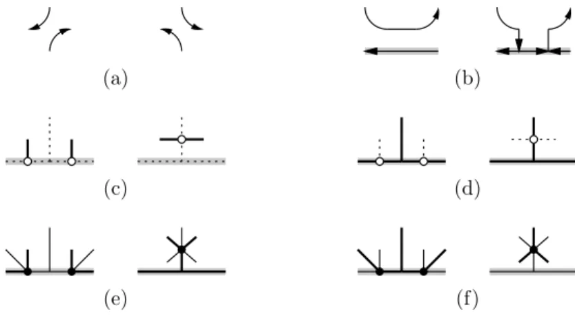
Any almost generic real trigonal curve can be perturbed to a generic one. 3.2.1. Two dessins are called equivalent if, after a homeomorphism of the underly-ing surfaces, they are connected by a finite sequence of isotopies and the followunderly-ing
elementary moves:
– monochrome modification, see Figure 1(a);
– creating (destroying) a bridge, see Figure 1(b), where a bridge is a pair of monochrome vertices connected by a real monochrome edge;
– ◦-in and its inverse ◦-out, see Figure 1(c) and (d); – •-in and its inverse •-out, see Figure 1(e) and (f).
(In the first two cases, a move is considered valid only if the result is again a dessin. In other words, one needs to check the absence of oriented monochrome cycles and
triangular regions other than disks.) An equivalence of two dessins in the same underlying surface D is called restricted if the homeomorphism is identical and the isotopies above can be chosen to preserve the pillars (as sets).
Figure 1. Elementary moves of dessins
3.2.2. Remark. In view of Condition 3.1(3) in the definition of trichotomic graph, any monochrome modification and creation/destruction of a bridge automatically respect the orientations of the edges involved, see Figure 1. This fact is in a contrast with the definition of equivalence of skeletons, see Subsection 5.3 below, where respecting a certain orientation is an extra requirement.
The following statement is proved in [2].
3.2.3. Proposition. Each dessin Γ is of the form ΓCfor some generic real trigonal curve C. Two generic real trigonal curves are deformation equivalent (in the class of almost generic real trigonal curves) if and only if their dessins are equivalent. ¤
3.2.4. The definition of the j-invariant gives one an easy way to reconstruct the topology of a generic real trigonal curve C ⊂ Σ from its dessin ΓC. Let π : Σ → B
and πC be as in Subsection 2.1. Topologically, the base B is the orientable double
of the underlying surface D of ΓC. Let Γ0 ⊂ B be the decorated preimage of ΓC,
see 3.1.1. Then B◦ = B r {×-vertices of Γ0} and the pull-back π−1
C (b) of a point b ∈ B◦ consists of three points in the complex affine line π−1(b) r E.
(1) If b is an inner point of a region of Γ0, the three points of π−1
C (b) form a
triangle ∆b with all three edges distinct. As a consequence, the restriction
of πC to the interior of each region of Γ0 is a trivial covering.
(2) If b belongs to a dotted edge of Γ0, the three points of π−1
C (b) are collinear.
The ratio (smallest distance)/(largest distance) is in (0, 1/2); it tends to 0 (respectively, 1/2) when b approaches a ×- (respectively, ◦-) vertex.
(3) If b belongs to a solid (bold) edge of Γ0, the three points of π−1
C (b) form an
isosceles triangle with the angle at the vertex less than (respectively, greater than) π/3. The angle tends to 0, π/3, or π when b approaches, respectively, a ×-, •-, or ◦-vertex.
The number of ◦-vertices of Γ0 is called the degree deg Γ of Γ. One has deg Γ =
0 mod 3, and −1
3.2.5. In view of 3.2.4(1), over the interior of each region R of the pull-back Γ0⊂ B
there is a canonical way to label the three sheets of C by 1, 2, 3, according to the increasing of the opposite side of the triangle ∆b over any point b ∈ R. This
labelling is obviously preserved by the real structure c : B → B and hence descends to the regions of Γ. The passage through an edge of Γ results in the following transformation:
– solid edge: the transposition (23); – bold edge: the transposition (12);
– dotted edge: the change of the orientation of ∆.
The transpositions above represent a change of the labelling rather than a nontrivial monodromy. Although the change of orientation of ∆ makes sense, its orientation itself is only well defined if B is of type I and a half of B is chosen.
3.2.6. The real components Γi of Γ are identified with the connected
compo-nents Bi of BR. The pull-back π−1C (b) of a real point b ∈ ∂D has three real points
if b is a dotted point or a ◦-vertex adjacent to two real dotted edges; it has two real points, if b is a×-vertex, and a single real point otherwise. A component Σi of ΣR
is orientable if and only if the corresponding real component Γi is even.
A component Bi is (anti-)hyperbolic (see 2.1) if and only if so is Γi. If Bi is
non-hyperbolic, its ovals and zigzags are represented by the maximal dotted segments of Γi, even and odd, respectively. The latter are also called ovals and zigzags of Γ.
4. Trigonal curves of type IB
In this section, we characterize the dessins of trigonal curves of type IBand study
their basic properties.
4.1. Canonical labelling. Let C be a non-hyperbolic trigonal curve of type IB,
and let C+⊂ C be the surface mapped generically one-to-one to B, see 2.4.4.
Let Γ ⊂ D be the dessin of C. Since C+ is c-invariant, each region R of Γ can
be labelled according to the label of the sheet of C+ over R, see 3.2.5. Then, each inner edge e of Γ can be labelled according to the label(s) of the adjacent regions.
The possible labels are as follows:
– an inner solid edge can be of type 1 or ¯1 (not 1); – an inner bold edge can be of type 3 or ¯3 (not 3); – an inner dotted edge can be of type 1, 2, or 3.
(One cannot distinguish types 2 and 3 along a solid edge or types 1 and 2 along a bold edge due to the relabelling mentioned above; in these cases, we assign to the edges types ¯1 and ¯3, respectively.) On the contrary, the same rule assigns a well defined label 1, 2, or 3 to each real edge e of Γ: the relabelling in 3.2.5 is compensated for by the discontinuity of C+ across BIm.
4.1.1. Lemma. A real solid edge cannot be of type 1; a real bold edge cannot be
of type 3.
Proof. Otherwise, the surface C+→ B would be two-sheeted over the regions of Γ
4.1.2. Theorem. A non-hyperbolic generic trigonal curve C is of type IB if and only if the regions of its dessin Γ ⊂ D admit a labelling which satisfies the following conditions:
(1) the region adjacent to a real solid (bold) edge is not of type 1 (respectively,
not of type 3);
(2) the two regions adjacent to an inner solid edge are either both of type 1 or
of distinct types 2 and 3;
(3) the two regions adjacent to an inner bold edge are either both of type 3 or
of distinct types 1 and 2;
(4) the two regions adjacent to an inner dotted edge are of the same type.
Proof. If C is of type IB, its labelling defined above does satisfy (1)–(4): Property
(1) is the statement of Lemma 4.1.1, and Properties (2)–(4) follow from 3.2.5. For the converse, lift the labelling to the preimage Γ0 ⊂ B of Γ, cf. 3.2.4, over
each region of Γ0 take the sheet selected by the labelling, and define C
+ as the
closure of the union of these sheets. Then, in view of (1)–(4), one has ∂C+= CIm, i.e., [CIm] = 0 ∈ H1(C; Z2), and C is of type IB due to Lemma 2.4.3. ¤
4.2. Dessins of type I. A dessin Γ equipped with a labelling satisfying Condi-tions 4.1.2(1)–(4) is said to be of type I. We assume the labelling extended to edges as explained in Subsection 4.1. Fix a dessin Γ of type I. Below, we discuss further properties of its labelling and extend it to some other objects related to Γ. 4.2.1. Lemma. The edges adjacent to an inner vertex are labelled as follows:
– ×-vertex: (1, 1);
– •-vertex: (1, ¯3, ¯1, 3, ¯1, ¯3);
– ◦-vertex: (3, 3, 3, 3) or (¯3, 1, ¯3, 2). ¤
4.2.2. Lemma. The edges adjacent to a real vertex are labelled as follows: – ×-vertex: both edges are of the same type 2 or 3;
– •-vertex: (2, ¯3, 1, 1) or (3, 3, ¯1, 2);
– ◦-vertex with real edges dotted: (3, 3, 3) or (1, ¯3, 2);
– ◦-vertex with real edges bold: all edges are of the same type 1 or 2. ¤ According to Lemmas 4.2.1 and 4.2.2, the two edges adjacent to a single×-vertex
are always of the same type. We assign this type to the vertex itself, thus speaking about×-vertices of type 1 (necessarily inner) or 2 or 3 (necessarily real).
4.2.3. Corollary. The two×-vertices bounding a single oval of Γ are of the same type, which can be 3 or 2. In the former case, all dotted edges constituting the oval are of type 3; in the latter case, the type of the edges alternates between 2 and 1 at each ◦-vertex. The two ×-vertices bounding a single zigzag of Γ are always of type 3, and so are all dotted edges constituting a zigzag. ¤
According to the types of the dotted edges constituting an oval, we will speak about ovals of type 3 and 2 (if all dotted edges are of type 3 or 2, respectively) and ovals of type ¯3 (if there are edges both of type 2 and 1). Note that ovals of type 2 are necessarily ‘short’, i.e., they contain no ◦-vertices, whereas each oval of type ¯3 necessarily contains a ◦-vertex.
4.2.4. Lemma. The real dotted edges constituting an odd (respectively, even)
hyperbolic component of Γ are all of type 3 (respectively, are all of the same type 3,
2, 1 or alternate between type 2 and 1 at each ◦-vertex).
Proof. Within each real dotted segment, the types of the edges either are const = 3
or alternate between 2 and 1 at each ◦-vertex. In the latter case, the number of vertices must be even. ¤
According to the types of the dotted edges constituting the component, we will speak about hyperbolic components of type 3, 2, 1, or ¯3. Note that components of type 2 or 1 do not contain ◦-vertices, whereas each component type ¯3 necessarily contains a ◦-vertex.
4.2.5. Lemma. The real part of Γ has no odd anti-hyperbolic components.
Proof. After destroying solid bridges and a sequence of •-ins along inner solid edges,
one can assume that the edges constituting an anti-hyperbolic component are all bold. They cannot be of type 3, see Lemma 4.1.1; hence, their types alternate between 1 and 2 at each inner bold edge attached to the component, and the component must be even. ¤
4.3. Unramified dessins of type I. A dessin is called unramified, if all its ×
-vertices are real. In other words, unramified are the dessins corresponding to maxi-mally inflected curves. In this subsection, we assume that Γ is an unramified dessin of type I.
4.3.1. Lemma. The dessin Γ has no solid or dotted edges of type 1.
Proof. A solid or dotted edge of type 1 would end at a×-vertex of type 1
(possi-bly, passing through a number of monochrome vertices), which would have to be inner. ¤
4.3.2. Lemma. Each •-vertex v ∈ Γ is real, and the edges adjacent to v are of
types (3, 3, ¯1, 2). The immediate essential neighbors of v in the real part of Γ are a ◦- and a×-vertex.
Proof. The first two statements follow from Lemmas 4.2.1, 4.2.2, and 4.3.1. If v
had another •-vertex as an immediate essential neighbor, the two vertices could be pulled in by a •-in transformation, producing an inner •-vertex. ¤
4.3.3. Corollary. The dessin Γ has no inner bold edges of type ¯3. ¤
4.3.4. Corollary. All edges adjacent to a single ◦-vertex of Γ are of the same
type. (Accordingly, we will speak about the type of a ◦-vertex.) A real ◦-vertex with real edges bold is of type 2; all other ◦-vertices are of type 3.
Proof. The types of edges adjacent to a ◦-vertex are listed in Lemmas 4.2.1 and
4.2.2, and all but a few possibilities are eliminated by Lemma 4.3.1. ¤ 4.3.5. Corollary. The dessin Γ has no ovals of type ¯3. ¤
4.3.6. Lemma. Let v ∈ Γ be a ◦-vertex of type 2. Then v is real, and the
immediate essential neighbors of v in the real part of Γ are two •-vertices.
Proof. According to Corollary 4.3.4, the vertex v is real and the real edges adjacent
to v are bold. Hence, the neighbors of v are either or •-vertices. If another ◦-vertex u (possibly, v itself) were a neighbor of v, the dotted segment connecting u
and v would contain a monochrome vertex with an inner bold edge of type ¯3 adjacent to it. This would contradict to Corollary 4.3.3. ¤
A pillar consisting of a ◦-vertex and pair of real bold segments connecting it to
•-vertices, as in Lemma 4.3.6, is called a jump. To each jump, we assign type 2,
according to the types of its ◦-vertex and bold edges.
4.3.7. Proposition. Any hyperbolic component of Γ is of type 3 or 2 (and in the
latter case it is free of ◦-vertices). Any anti-hyperbolic component of Γ is formed by solid edges and solid monochrome vertices.
Proof. As in the proof of Lemma 4.2.5, if an anti-hyperbolic component has a bold
edge, one can assume all edges of this component bold. Any hyperbolic component of type ¯3 or any real component with all edges bold would have an inner bold edge of type ¯3 attached to it; this contradicts to Corollary 4.3.3. Similarly, any hyperbolic component of type 1 would have an inner dotted edge of type 1 attached to it; this contradicts to Lemma 4.3.1. ¤
The following theorem summarizes the results of this section. 4.3.8. Theorem. Let Γ be an unramified dessin of type I. Then
(1) the pillars of Γ are ovals, zigzags, jumps, and hyperbolic components; (2) each pillar has a well defined type, 2 or 3, all jumps being of type 2 and all
zigzags being of type 3;
(3) pillars of type 2 are interconnected by inner dotted edges of type 2; these
edges, as well as pillars of type 2 other than jumps, are free of ◦-vertices;
(4) pillars of type 3 are interconnected by inner dotted edges of type 3 or pairs
of such edges attached to an inner ◦-vertex each;
(5) the following parity rule holds: along each real component of Γ, the types
of the pillars alternate. ¤
4.4. Complex orientations. Recall that the real part CRof any connected
alge-braic curve C of type I admits a distinguished pair of opposite orientations, called
complex orientations, which are induced on the common boundary CR= ∂C± by
the complex orientations of the two halves C± of C.
Let C ⊂ Σ be a nonsingular real trigonal curve over a base B of type I. Consider the set B ⊂ BRof real fibers of Σ that intersect CRin a single point each (counted
with multiplicity). Denote by ¯B the closure of B, and let ¯L be the restriction to ¯B
of the real ruling π : ΣRr ER→ BR. It is a real affine line bundle. Any orientation
of CRinduces in an obvious way an orientation of the restriction ¯L|BrB¯ .
4.4.1. Definition. For a non-hyperbolic curve C, an orientation of CR is called quasi-complex if the induced orientation of ¯L|BrB¯ extends to ¯L and, with respect
to some complex orientation of BR, the restriction of the projection πC: CR→ BR
is of degree +1 over each component of BR.
4.4.2. Remark. Denote by Z the projection to BRof the union of all zigzags and
real vertical flexes of CR. Then, CRadmits a quasi-complex orientation if and only
if, over each component B0 of B
Rr Z, the total number of ovals of CR and points
4.4.3. Proposition. Any complex orientation of a non-hyperbolic trigonal curve
of type I is quasi-complex.
Proof. For the extension of the orientation to ¯L one can mimic the proof found in [3].
New is the case of a component of BRthat lies entirely in B. The orientability of ¯L
over such a component follows from Lemma 4.2.5.
For a non-hyperbolic trigonal curve C of type I, the complement C r πC−1(BR)
splits into four ‘quoters’ C±
± = C±∩ C±. Since both C+ and C− are c-invariant,
whereas C+and C−are interchanged by c, any point of C
Rover B is in the common
part of the boundaries ∂C−±. Thus, assuming that πC(C−+) = B+, one concludes
that the map πC: CR→ BRis of degree +1. ¤
4.4.4. Proposition. Any hyperbolic trigonal curve C is of type IB. Such a curve is of type I if and only if its base B is of type I. In this case, with respect to some complex orientations of CRand BR, one has (πC)∗[CR] = 3[BR].
Proof. The first statement is a tautology, and the second one follows immediately
from Lemma 2.4.2. For the third statement, it suffices to observe that, in the hyperbolic case, the halves C± are the pull-backs π−1
C (B±). ¤
5. Skeletons
Unramified dessins of type I can be reduced to somewhat simpler objects, the so called skeletons, which are obtained by disregarding all but dotted edges. The prin-cipal result of this section is Theorem 5.4.6 describing maximally inflected trigonal curves of type I in terms of skeletons.
Throughout this section, we assume that the underlying surface D is orientable, in other words, the base B of the ruling is of type I and, hence, trigonal curves of type IB are those of type I.
5.1. Abstract skeletons. Consider an embedded (finite) graph Sk ⊂ ¯D in a
compact surface ¯D. We do not exclude the possibility that some of the vertices
of Sk belong to the boundary of ¯D; such vertices are called real. The set of edges
at each real (respectively, inner) vertex v of Sk inherits from ¯D a pair of opposite
linear (respectively, cyclic) orders. The immediate neighbors of an edge e at v are the immediate predecessor and successor of e with respect to (any) one of these orders. A first neighbor path in Sk is a sequence of oriented edges of Sk such that each edge is followed by one of its immediate neighbors.
Below, we consider graphs with connected components of two kinds: directed and undirected. We call such graphs partially directed. The directed and undirected parts of a partially directed graph Sk are denoted by Skdir and Skud, respectively.
Accordingly, we speak about directed and undirected vertices of these graphs. 5.1.1. Definition. Let ¯D be a compact orientable surface with nonempty
bound-ary. An abstract skeleton is a partially directed embedded graph Sk ⊂ ¯D, disjoint
from the boundary ∂ ¯D except for some vertices, and satisfying the following
con-ditions:
(1) at each vertex of Skdir, the directions of adjacent edges alternate;
(2) each real directed vertex has odd valency, thus being a source or a sink ; (3) each source is monovalent;
(5) each boundary component l of ¯D has a vertex of Sk and is subject to the parity rule: directed and undirected vertices alternate along l;
(6) if a component R of the cut ¯DSk has a single source in the boundary ∂R,
then R is a disk.
5.2. Admissible orientations.
5.2.1. Definition. Let Sk ⊂ ¯D be an abstract skeleton. An orientation of Skud is
called admissible if, at each vertex, no two incoming edges are immediate neighbors. An elementary inversion of an admissible orientation is the reversal of the direction of one of the edges so that the result is again an admissible orientation.
5.2.2. Proposition. Any abstract skeleton Sk has an admissible orientation. Any
two admissible orientations of Sk can be connected by a sequence of elementary inversions.
This statement is proved after Proposition 5.2.3 below. Due to the existence of admissible orientations, all undirected edges of an abstract skeleton Sk ⊂ ¯D can
be divided into two groups: triggers and diodes, the latter being those that have the same direction, called natural, in all admissible orientations of Sk. On the contrary, each trigger has two states (orientations); each state can be extended to an admissible orientation of the skeleton.
5.2.3. Proposition. Let Sk ⊂ ¯D be an abstract skeleton and e1, e2 two distinct triggers. Then, out of the four states of the pair e1, e2, at least three extend to an admissible orientation.
Proof of Propositions 5.2.2 and 5.2.3. To construct an admissible orientation of Sk,
choose an undirected edge e1, orient it arbitrarily, and call the result ~e1 the first anchor. For each first neighbor path starting at ~e1, orient each edge e0 of the path
in the direction from ~e1, i.e., assign to e0 the orientation induced from the path.
If the partial orientation thus obtained is consistent, keep it; otherwise, disregard this orientation and repeat the procedure starting from the first anchor −~e1, i.e.,
the same edge e1 with the orientation opposite to the originally chosen one.
We assert that at least one of the anchors ~e1 and −~e1 results in a consistent
partial orientation. Indeed, otherwise there are two oriented edges e0, e00, a pair of
first neighbor paths γ0
±starting at~e1and ending at ±e0, and a pair of first neighbor
paths γ00
±starting at −~e1and ending at ±e00. Then, the sequence γ+0 , γ−0−1, γ+00, γ−00−1
gives rise to a first neighbor cycle.
If there is an edge e2that has not yet been assigned an orientation, orient it and
repeat the procedure starting from the second anchor ~e2or −~e2, whichever works.
Clearly, the new orientation is consistent with the one obtained in the previous step. Continue this procedure (selecting anchors and extending their orientation) until the whole undirected part of Sk is exhausted.
Notice that any admissible orientation of Sk can be obtained by this procedure with an appropriate choice of the anchors.
For the uniqueness up to elementary inversions, fix an admissible orientation o obtained from a sequence of anchors ~e1,~e2, . . . and consider another admissible
orientation o0. Among the first neighbor paths starting at ~e
1 and ending at an
edge e0 whose o0-orientation differs from o, choose a maximal one. Then, reversing
Repeat this procedure to switch to o the orientations of all edges reachable from
~e1; then continue with ~e2, etc.
To prove Proposition 5.2.3, note that an undirected edge e of Sk is a trigger if and only if both~e and −~e can be chosen for an anchor. Choose a state~e1of e1. If e2
can be reached (by a first neighbor path) stating from~e1, then e2cannot be reached
from −~e1, as otherwise the two orientations induced on e2 would coincide (no first
neighbor cycles) and hence e2 would be a diode. Thus, one can assume that e2 is
not reachable from~e1, and three admissible orientations can be constructed starting
from the anchors ~e1, ±~e2, . . . and −~e1, . . . . ¤
Figure 2. A diod
5.2.4. Remark. If an abstract skeleton Sk ⊂ ¯D does not have cycles, then any
undirected edge of Sk is a trigger. Note however that in general diods do exist, see, e.g., the fragment shown in Figure 2. (This fragment can easily be completed to a skeleton without inner vertices.) Alternatively, one can consider a skeleton with a monovalent inner vertex v: the only edge adjacent to v is its own immediate neighbor; hence it cannot be oriented towards v.
5.3. Equivalence of abstract skeletons. Two abstract skeletons are called
equivalent if, after a homeomorphism of underlying surfaces, they can be connected
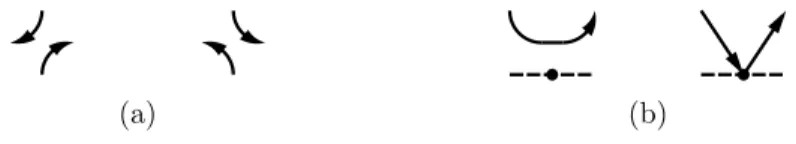
by a finite sequence of isotopies and the following elementary moves, cf. 3.2.1: – elementary modification, see Figure 3;
– creating (destroying) a bridge in Skud, see Figure 3; the vertex shown in the
figure can be inner or real, and the dotted lines represent other edges of Skud
that may be present.
(A move is valid only if the result is again an abstract skeleton.) It is understood that an elementary move does not mix Skdir and Skud and, when acting on Skdir,
a move must respect the prescribed orientations (as shown in the figures), thus defining an orientation on the resulting directed part. On Skud, a move is required
to respect some admissible orientation of the original skeleton and take it to an admissible orientation of the result. Note that, in a contrast to the definition of equivalence of dessins, see 3.2.1, respecting a certain orientation, either prescribed or admissible, is an extra requirement here, cf. Remark 3.2.2.
An equivalence of two abstract skeletons in the same surface and with the same set of vertices is called restricted if the homeomorphism is identical and the isotopies above can be chosen identical on the vertices.
5.3.1. Remark. For Skud, the orientation condition in the definition above is
restrictive only if all edges involved are diodes; otherwise, a required admissible orientation does exist due to Proposition 5.2.3. For creating a bridge, it would even suffice to assume that at least one of the immediate neighbors of the bridge created is a trigger. In particular, if ¯D is a disk, then any elementary move is allowed, see
Remark 5.2.4.
5.4. Dotted skeletons. From now on, for simplicity, we confine ourselves to dessins without anti-hyperbolic components. All such components would be mono-chrome, see Proposition 4.3.7, and thus could easily been incorporated using the concept of (partial) reduction, see [2].
5.4.1. Intuitively, the dotted skeleton is obtained from a dessin Γ by disregarding all but dotted edges and patching the latter through all ◦-vertices. According to Theorem 4.3.8, each inner dotted edge of type 2 retains a well defined orientation, whereas an edge of type 3 may be broken by ◦-vertex, and for this reason, its orientation may not be defined. As types do not mix, edges and pillars of types 2 and 3 would form separate components of the skeleton.
5.4.2. Definition. Let Γ ⊂ D be an unramified dessin of type I without anti-hyperbolic components. The (dotted) skeleton of Γ is the partially directed graph Sk = SkΓ ⊂ ¯D obtained from Γ as follows:
– contract each pillar to a single point and declare this point a vertex of Sk; – patch each inner dotted edge through its ◦-vertex, if there is one, and declare
the result an edge Sk;
– let Skdir and Skud be the images of the edges and pillars of type 2 and 3,
respectively, each edge of type 2 inheriting its orientation from Γ.
Here, ¯D is the surface obtained from D by contracting each pillar to a single point.
5.4.3. Proposition. The skeleton Sk of a dessin Γ as in Definition 5.4.2 is an
abstract skeleton in the sense of Definition 5.1.1.
Proof. Properties 5.1.1(1)–(3) follow immediately from Theorem 4.3.8. Each
com-ponent of ∂ ¯D has a vertex of Sk due to our assumption that Γ has no anti-hyperbolic
component, and the parity rule in 5.1.1(5) is a consequence of Theorem 4.3.8(5). Property 5.1.1(6) is merely a restatement of requirement (8) in the definition of trichotomic graph, see Subsection 3.1.
For 5.1.1(4), apply a sequence of ◦-outs along type 3 dotted edges to convert Γ to a dessin Γ0 with the same skeleton Sk and all ◦-vertices real. The orientation
of dotted edges of Γ0 induces the prescribed orientation of Sk
dir and an admissible
orientation of Skud, the ◦-vertices of Γ0residing in the real dotted edges connecting
outgoing inner dotted edges and/or×-vertices. Thus, a first neighbor cycle of Sk
would give rise to an oriented dotted cycle of Γ0, which contradicts to the definition
of dessin, see 3.2. Finally, the inner vertices of Sk are the images of hyperbolic components of Γ, which are necessarily adjacent to inner dotted edges. ¤
5.4.4. Proposition. Any abstract skeleton Sk ⊂ ¯D is the skeleton of a certain dessin Γ as in Definition 5.4.2; any two such dessins can be connected by a sequence of isotopies and elementary moves, see 3.2.1, preserving the skeleton.
5.4.5. Proposition. Let Γ1, Γ2⊂ D be two dessins as in Definition 5.4.2; assume that Γ1 and Γ2 have the same pillars. Then, Γ1 and Γ2 are related by a restricted equivalence if and only if so are the corresponding skeletons Sk1and Sk2.
Propositions 5.4.4 and 5.4.5 are proved in Subsections 5.5 and 5.6. Here, we state the following immediate consequence.
5.4.6. Theorem. There is a canonical bijection between the set of equivariant
fiberwise deformation classes of maximally inflected type I real trigonal curves without anti-hyperbolic components and the set of equivalence classes of abstract skeletons. ¤
5.5. Proof of Proposition 5.4.4. The underlying surface D containing Γ is the orientable blow-up of ¯D at the vertices of Sk: each inner (boundary) vertex v is
replaced with the circle (respectively, segment) of directions at v. The circles and segments inserted are the pillars of Γ. Each source gives rise to a jump and is decorated accordingly; all other pillars consist of dotted edges (the ◦-vertices are to be inserted later, see 5.5.1) with ×-vertices at the ends. The proper transforms
of the edges of Sk are the inner dotted edges of Γ.
5.5.1. The blow-up produces a certain dotted subgraph Sk0 ⊂ D. Choose an
admissible orientation of Sk, see Proposition 5.2.2, regard it as an orientation of the inner edges of Sk0, and insert a ◦-vertex at the center of each real dotted segment connecting a pair of outgoing inner edges and/or×-vertices.
5.5.2. Let ¯U ⊂ ¯D be a closed regular neighborhood of Skdir disjoint from Skud,
and U ⊂ D be the preimage of ¯U . Shrink U along ∂D so that the boundary ∂U
contains the •-vertices and take for the inner solid edges of Γ the connected com-ponents of the inner part of ∂U , defining real solid edges and monochrome vertices accordingly. Note that, in view of Condition 5.1.1(4), each connected component of the inner part ∂U r ∂D is an interval rather than a circle, as a circle in ∂U disjoint from ∂D would contract to a first neighbor cycle in Skdir.
5.5.3. At this point, the closure of the complement D r U should be the union of the type 3 regions of the dessin in question, and the cut (D r U )Sk0 should contain
inner bold edges only. Let R be a region of this cut. The •- and ◦-vertices of Γ define germs of bold edges at the boundary ∂R; due to the parity rule 5.1.1(5), incoming and outgoing bold edges alternate along each component of ∂R. Consider a disk B2
with a distinguished oriented diameter d and let ϕ : ∂R → ∂B2 be an orientation
preserving covering taking the incoming/outgoing bold edges to the corresponding points of d ∩ ∂B2. In view of 5.1.1(6), the map ϕ extends to a ramified covering
¯
ϕ : R → B2, which can be assumed regular over d, and it suffices to take for the
inner bold edges of Γ the components of the pull-back ¯ϕ−1(d). This completes the
construction of a dessin extending Sk0.
5.5.4. For the uniqueness, first observe that a decoration of Sk0 with ◦-vertices is
unique up to isotopy and ◦-ins/◦-outs along dotted edges. Indeed, assuming all
◦-vertices real, each such decoration is obtained from a certain admissible
Proposition 5.2.2, and an elementary inversion results in a ◦-in followed by a ◦-out at the other end of the edge reversed. Thus, the distribution of the ◦-vertices can be assumed ‘standard’.
5.5.5. The union of the solid edges of any dessin Γ extending Sk0is the inner part of the boundary of the shrunk preimage U ⊂ D of a certain closed neighborhood ¯U
of Skdir, cf. 5.5.2. (This neighborhood U is the union of the type 2 regions of Γ,
see Theorem 4.3.8.) We assert that, for each Γ, there is a decreasing family of neighborhoods Ut, t ∈ [0, 1], U0 = U , Ut0 ⊂ Ut00 for t0 > t00, composed of isotopies
and finitely many elementary modifications of the boundary and such that U1is a
regular neighborhood, see 5.5.2, and, for each regular value t ∈ [0, 1], replacing the solid edges of Γ with the inner part of ∂Utresults in a valid dessin. Indeed, each
component of the cut USk0 is a disk with holes and handles, and it can be simplified
by the following operations:
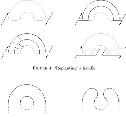
– first, ‘replant’ each handle by two monochrome modifications, see Figure 4; – next, eliminate each hole by a monochrome modification, see Figure 5; – finally, by a number of monochrome modifications, cut the resulting surface
into triangles, see 3.1(8).
It is a routine to check that each monochrome modification used can be chosen to involve a pair of distinct solid edges (due to 3.1(8), unless the component in question already is a triangle, it has at least two solid edges in the boundary) and that, under this assumption, each intermediate trichotomic graph is a valid dessin.
Figure 4. ‘Replanting’ a handle
5.5.6. Since any two regular neighborhoods of Skdir are isotopic, it remains to
consider two dessins that differ by bold edges only. Any collection of inner bold edges of a valid dessin is obtained by the construction of 5.5.3, from an appropriate ramified covering ¯ϕ : R → B2(cf. the passage from a dessin to a j-invariant in [2]).
Since the restrictions ϕ : ∂R → ∂B2corresponding to the two dessins are homotopic,
the extension is unique up to homotopy in the class of ramified covering, see [4]. Hence, the two dessins are related by a sequence of bold modifications. ¤
It is items 5.5.3 and 5.5.6 in the proof why we had to exclude from the consid-eration the case of the base curve of type II, i.e., nonorientable ¯D.
5.6. Proof of Proposition 5.4.5. The ‘only if’ part is obvious: an elementary move of a dessin either leaves its skeleton intact or results in its elementary modi-fication; in the latter case, a pair of edges of the same type is involved, i.e., either both directed (and then the orientation is respected) or both undirected (and then some admissible orientation is respected, see 5.5.1).
For the ‘if’ part, consider the skeleton Sk at the moment of a modification. It can be regarded as the skeleton of a dessin with inner monochrome vertices allowed (see admissible trichotomic graphs in [2]), and, repeating the proof of Proposition 5.4.4, one can see that Sk does indeed extend to a certain dessin. The extension remains a valid dessin Γ before the modification as well. Hence, due to the uniqueness given by Proposition 5.4.4, one can assume that the original dessin is Γ, and then the modification of the skeleton is merely an elementary modification of Γ.
Destroying a bridge of a skeleton is the same as destroying a bridge of the corre-sponding dessin, and the inverse operation of creating a bridge extends to a dessin equivalent to the original one due to the uniqueness given by Proposition 5.4.4. ¤
6. The case of the rational base
In this section we prove Theorems 1.1.1 and 1.1.2 and attempt a constructive description of maximally inflected trigonal curves of type I in rational ruled surfaces. Note that, in the settings of Theorems 1.1.1 and 1.1.2, each skeleton Sk is a forest in the disk, and all vertices of Sk are on the boundary.
6.1. Proof of Theorem 1.1.1. The ‘only if’ part is given by Proposition 4.4.3. For the ‘if’ part, consider a regular neighborhood V ⊂ B of BR. Under the
as-sumptions on the orientation, the germ C0 = π−1
C (V ) is separated by CR, cf. e.g.
[6, Proof of Theorem 1.3.A]. On the other hand, since the covering πC: C → B is
unramified over the two disks B rBR, the curve C is obtained from C0by attaching
six disks; hence it remains separated. ¤
6.2. Proof of Theorem 1.1.2. Consider a trigonal curve C0 as in the statement,
and let Sk0 be the associated skeleton in the disk ¯D ' P1/c. Destroying all bridges
(see Remark 5.3.1), one can assume that the valency of each vertex of Sk0is at most one, i.e., each undirected component of Sk0 is either an isolated vertex (zigzag) or a single edge connecting two vertices (ovals). Ignore the zigzags: their position is uniquely recovered by the parity rule 5.1.1(5). Then, Sk0 turns into a collections of
disjoint chords in the disk ¯D, directed and undirected, connecting points in ∂ ¯D of
three types: sources, sinks, and undirected vertices.
Let Sk00 be the skeleton associated to the other curve C00 with the same
modi-fications as above. Identify the vertices of Sk00 with those of Sk0 according to the homeomorphism of the real parts. Let l be a shortest chord of Sk0, i.e., such that
one of the two arcs constituting ∂ ¯D r l is free of vertices of the skeletons.
Perform-ing, if necessary, an elementary modification, one can assume that l is also an edge of Sk00. Remove the part of the disk cut off by l and proceed by induction, ending up with a pair of empty skeletons, which are obviously equivalent. Thus, Sk00 is equivalent to Sk0, and Propositions 5.4.4 and 5.4.5 imply the theorem. ¤
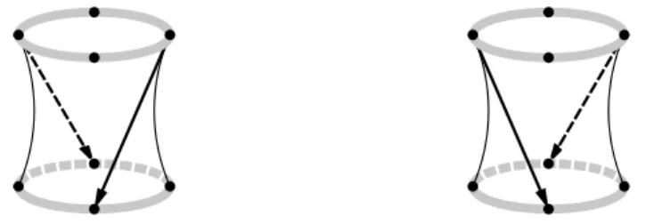
6.2.1. Remark. Theorem 1.1.2 does not extend to not maximally inflected curves, even of type I; an example of two non-equivalent M -curves with isotopic real parts is found in [2]. Nor does the theorem extend to the case of a base of positive genus: the two skeletons shown in Figure 6 (where ¯D is a cylinder) are obviously not
related by restricted equivalence, as the orientations shown prohibit any elementary modification. One can easily construct pairs of skeletons with isomorphic real parts and not related by any equivalence, restricted or not.
Figure 6. Nonequivalent skeletons with the same real part
6.3. Blocks. In this section, we make an attempt of a constructive description of the real parts of maximally inflected type I trigonal curves over the rational base. 6.3.1. Definition. A type I dessin Γ in the disk is called a block if Γ is unramified and has no inner dotted edges of type 3.
It follows from Theorem 4.3.8 that all vertices of any block Γ are real, all its ovals are of type 2, and all its zigzags are ‘short’, i.e., each zigzag contains a single ◦-vertex. In particular, the real part of Γ consists of n = 1
3deg Γ ovals
and n jumps, which are intermitted with 2n zigzags; the position of the zigzags is uniquely determined by the parity rule 4.3.8(5). Blocks are easily enumerated by the following statement.
6.3.2. Proposition. Let n > 1 be an integer, and let O, J ⊂ S1 = ∂D be two disjoint sets of size n each. Then, there is a unique, up to restricted equivalence, block Γ ⊂ D of degree 3n with an oval about each point of O, a jump at each point of J, and a zigzag between any two points of O ∪ J (and no other pillars).
Proof. Fix a bijection between J and O and connect each point of J to the
corre-sponding point of O by a directed chord. Whenever two chords intersect, resolve the crossing respecting the orientation. Add to the resulting directed graph an isolated vertex between any two points of O ∪ J. The result is an abstract dotted skeleton; due to Proposition 5.4.4, it extends to a block. The uniqueness is given by Theorem 1.1.2. ¤
Proposition 6.3.2 and Theorem 4.3.8 provide a complete description of the real parts of maximally inflected type I trigonal curves over P1. Realizable are the real
Proposition 6.3.2, and perform a sequence of junctions converting the disjoint union of disks to a single disk.
6.3.3. Remark. The description of maximally inflected curves of type I given above, in terms of junctions, is similar to that of M -curves, see [2]. However, unlike the case of M -curves, in general a decomposition of an unramified dessin of type I into a junction of blocks is far from unique.
6.3.4. Remark. Combining blocks, one can also obtain a great deal of maximally inflected type I trigonal curves over irrational bases. However, in the case of the base of positive genus, this construction is no longer universal: there are unramified dessins of type I that cannot be cut into disks, see, e.g., the skeletons in Figure 6.
Appendix A
In the main part of the paper, we consider nonsingular trigonal curves up to fiberwise deformation equivalence, i.e., we do not allow a pair of simplest (type
˜ A∗
0) singular fibers to merge into a vertical flex. This notion, natural in the
frame-work of trigonal curves, is not quite usual in general theory of nonsingular algebraic curves in surfaces, where a less restrictive relation, the so called rigid isotopy, is used. We reinterpret this notion in terms of dessins and prove that any non-hyperbolic nonsingular real trigonal curve of type IB is rigidly isotopic to a maximally inflected
one, see Theorem A.2.5.
A.1. Rigid isotopies and week equivalence. Keeping the conventional termi-nology, we define rigid isotopy of nonsingular real trigonal curves as the equivalence relation generated by real isomorphisms and equivariant deformations in the class of nonsingular (not necessarily almost-generic) trigonal curves. Note that, in spite of the name ‘isotopy’, the underlying surface Σ and the base B are still not as-sumed fixed: the complex structure is also subject to deformation. Without this convention, Proposition A.1.2 below would not hold.
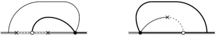
Intuitively, the new notion differs from the deformation equivalence by an extra pair of mutually inverse operations: straightening/creating a zigzag, the former consisting in bringing the two vertical tangents bounding a zigzag together to a single vertical flex and pulling them apart to the imaginary domain. On the level of dessins, these operations are shown in Figure 7.
A.1.1. Definition. Two dessins are called weakly equivalent if they are related by a sequence of isotopies, elementary moves (see 3.2.1), and the operations of
straightening/creating a zigzag consisting in replacing one of the fragments shown
in Figure 7 with the other one.
Figure 7. Straightening/creating a zigzag