THE IMPACT OF ENVIRONMENTAL EFFICIENCY ON BILATERAL TRADE: A PANEL DATA
ESTIMATION OF GRAVITY MODEL
A Master’s Thesis by SEDA MEYVECİ Department Of Economics Bilkent University Ankara January 2009
THE IMPACT OF ENVIRONMENTAL EFFICIENCY ON BILATERAL TRADE: A PANEL DATA
ESTIMATION OF GRAVITY MODEL
The Institute of Economics and Social Sciences of
Bilkent University
by
SEDA MEYVECİ
In Partial Fulfillment of the Requirements for the Degree of MASTER OF ARTS in THE DEPARTMENT OF ECONOMICS BİLKENT UNIVERSITY ANKARA January 2009
I certify that I have read this thesis and have found that it is fully adequate, in scope and in quality, as a thesis for the degree of Master of Arts in Economics.
--- Assoc. Prof. Fatma Taşkın Supervisor
I certify that I have read this thesis and have found that it is fully adequate, in scope and in quality, as a thesis for the degree of Master of Arts in Economics.
--- Assoc. Prof. Osman Zaim Examining Committee Member
I certify that I have read this thesis and have found that it is fully adequate, in scope and in quality, as a thesis for the degree of Master of Arts in Economics.
--- Assoc. Prof. Elif Akbostancı Examining Committee Member
Approval of the Institute of Economics and Social Sciences
--- Prof. Dr. Erdal Erel
ABSTRACT
THE IMPACT OF ENVIRONMENTAL EFFICIENCY ON BILATERAL TRADE: A PANEL DATA
ESTIMATION OF GRAVITY MODEL
Meyveci, Seda
M.S., Department of Economics Supervisor: Assoc. Prof. Fatma Taşkın
January 2009
In this study the role of environmental efficiency in the determination of bilateral trade flows is empirically examined by using Gravity Model for a panel data for 1971 to 2003. Although there are a number of empirical studies that analyze the relationship between environment and trade, most of them show insignificant relationship between environmental regulations and trade. Their differences are mostly due to the use of stringency indicators that are computed with different methods. This study, unlike previous studies, computes the environmental efficiency as a hyperbolic measure of technical efficiency in a non-parametric piecewise linear technology, with a production plan that maximizes the desirable outputs while simultaneously minimizing the resource use and pollution emission. The relationship between bilateral exports and environmental conditions measured as environmental efficiency index is investigated. The empirical results indicate that although there is no significant relationship between exports of a country and its own environmental efficiency index, there is a strong and robust positive effect of the partner country's environmental efficiency index.
ÖZET
ÇEVRESEL ETKİNLİĞİN KARŞILIKLI TİCARETTE ROLÜ: ÇEKİM MODELLERİNİN PANEL ANALİZİ
Meyveci, Seda
Yüksek Lisans, İktisat Bölümü Tez Danışmanı: Doç. Dr. Fatma Taşkın
Ocak 2009
Bu tezde, Çekim Model kullanılarak karşılıklı ticarette çevresel etkinliğin rolü, 1971 2003 yılları arası panel analiz yapılarak amprik olarak incelenmiştir. Literatürde, her ne kadar çevre ile ticaret arasındaki ilişkiyi araştıran çok farklı çalışmalara rastlamak mümkün olsa da, ampirik çalışmaların çoğunda çevre mevzuatı ile ticaret arasında zayıf yönlü bir ilişki kurulduğu görülmüştür. Bu tezde, diğer çalışmaların aksine, çevresel etkinlik “non parametrik parçalı linear” teknolojideki teknik etkinliğin hiperbolik bir ölçümü olarak hesaplanmıştır. Bu methodla kaynak kullanımını ve kirliliği minimize eden aynı zamanda üretimi maksimize eden üretim planı varsayımı altında ikili ihracat ve çevresel şartlar arasındaki söz konusu ilişkiyi ölçebilmeye yarayan çevresel etkinlik endeksi bulunmuştur. Elde edilen amprik sonuçlardan, bir ülkenin ihracatı ile çevresel etkinlik endeksi arasında belirgin bir ilişki olmasa da, diğer ülkenin çevresel etkinlik endeksinde güçlü bir pozitif etkinin olduğu sonucuna ulaşılmıştır.
ACKNOWLEDGEMENTS
I am grateful to my advisor Associate Professor Fatma Taşkın for her invaluable guidance and encouragement.
I want to thank my examining committee members, Associate Professor Osman Zaim and Associate Professor Elif Akbostancı for their valuable comments.
I want to thank Professor Hakan Berument and Dr. Eray Yücel for their generous help in processing the data.
I want to thank all my colleagues at Economic Research Department of Vakıfbank for their generous help and my supervisor Cem Eroğlu for encouraging me in my graduate study.
I also thank to all my friends and especially Mehmet Özer, Seda Köymen, Sevcan Yeşiltaş, Vesile Kutlu and Zeynep Burcu Bulut for their friendship and support during my graduate study at Bilkent. I am also grateful to Mehmet Doğanay who supports and encourages me a lot.
The financial support of TUBITAK during my studies is gratefully acknowledged.
Finally, I thank to my family and especially my mother Kader Meyveci, father Ruknettin Meyveci and sister Kıvılcım Eda Meyveci for supporting me in all stages of my education.
TABLE OF CONTENTS
ABSTRACT………...…………... iii
ÖZET……… iv
ACKNOWLEDGEMENTS………...………….. v
TABLE OF CONTENTS………. vi
LIST OF TABLES………... viii
LIST OF GRAPH………. ix
CHAPTER I: INTRODUCTION………...………....…………. 1
CHAPTER II: LITERATURE REVIEW OF GRAVITY MODEL OF TRADE………... 8
2.1 Theoretical Studies of Gravity Model ……….. 8
2.2 Empirical Applications of Gravity Model ……… 11
CHAPTER III: THE RELATIONSHIP BETWEEN TRADE AND ENVIRONMENT………... 15
3.1 Theoretical Studies ……….……….………… 15
3.2 Empirical Applications of Gravity Model ………... 20
CHAPTER IV: ENVIRONMENTAL EFFICIENCY INDEX…………... 25
4.1 Literature Review…..………. 25
4.2 Model……….……… 27
4.2.1 The Parent Technology………. 28
4.3 Data……… 36
4.4 Results………....……… 37
CHAPTER V: ESTIMATION OF GRAVITY MODEL WITH ENVIRONMENTAL EFFICIENCY INDEX……… 46
5.1 Data……….. 46
5.2 Model……….……….. 46
5.3 Empirical Results………. 48
5.4 The Extensions of Gravity Equation with New Variables and Dummies………. 52
5.5 Robustness Check……… 56
5.5.1 Endogenity Problem between Exports and Income Levels of the Countries……… 56
5.5.2 Restrictions on the coefficients of Environmental Efficiency Index………... 57
CHAPTER VI: CONCLUSION ………. 57
BIBLIOGRAPHY……… 59
APPENDICES……..……….... 62
APPENDIX A………... 67
APPENDIX B…..………... 73
LIST OF TABLES
1. Table 7.1: Efficiency index under strong disposability of undesirable Outputs √Г………….…...
76
2. Table 7.2: Efficiency Index under weakly disposability of undesirable outputs √Ω……….
79
3. Table 7.3: Table 7.3 Environmental Efficiency Index H=√Γ/√Ω……. 82
Table 7.3.1 Geometric Mean of Environmental Efficiency Index H=√Γ/√Ω……… 85
4. Table 7.4 Output Loss from Imposing Weak Disposability of Pollutants (1-H)×GDP (billions US $)……….. 86
5. Table 7.5 Pooled OLS Results……….. 87
6 Table 7.6 Estimated Models with Country Fixed Effect……….. 88
7. Table 7.7 Diagnostic Test Results……….. 89
8. Table7.8 Extension of the Model………... 90
9. Table 7.9 Estimated Models with Random Effects……… 91
10. Table 7.10 Estimated Models with Instrumental Variables…………... 92
LIST OF GRAPHS
1. Graph 1: Representations of Technology………... 29
2. Graph 2: Disposability of Inputs……… 31
3. Graph 3: Disposability of Outputs………. 32
4. Graph 4: Output sets for strongly and weakly disposable undesirable
outputs……… 34
5. Graph 5: Comparison of mean efficiency and total pollution per
output………. 40
6 Graph 6: Comparison of mean efficiency and total output per unit of
capital………. 41
7. Graph 7: Comparison of mean efficiency for developed and
developing countries……….. 43
8. Graph 8: Comparison of total pollution per unit of output for developed and developing countries……….. 44
CHAPTER I
INTRODUCTION
Human beings have made major impact on the world's ecosystems. A century ago, human use of the planet's resources was much less, and not perceived as destructive. However, today the damage can be seen in the form of global warming, air pollution, acid rains, new diseases and ecological collapse. The threat of the environmental pollution is one of the most important dangers of the world, and human activity is responsible for most of this damage. Rapid growth in industrial and agricultural production and increasing life standards are disrupting the environment and creating a threat on human beings.
Today global warming is most apparent environmental damage. According to Gillett, et al (2008) report1 the increase in atmospheric greenhouse gases due to human activity has caused most of the observed warming since the start of the industrial era and the contribution of human activity to global
1 Gillett, Nathan P, Dáithí A. Stone, Peter A. Stott, Toru Nozawa, Alexey Yu. Karpechko, Gabriele C. Hegerl, Michael F. Wehner & Philip D. Jones (2008). "Attribution of polar warming to human influence". Nature Geoscience 1: 750. doi:10.1038/ngeo338. http://www.cru.uea.ac.uk/~nathan/pdf/ngeo338.pdf.
warming is obvious in the last fifty years. Moreover, according to the report of Climate Change (2007): The Physical Science Basis, Intergovernmental Panel on Climate Change2, global temperatures on both land and sea have increased by 0.75 °C (1.35 °F) relative to the period 1860--1900 and by this speed it will not be too long for human to face with flood and drought. Furthermore, global warming as its name suggests is a global issue that one country having rules that protect the environment and the others not having rules will not help to clean the environment. Hence, environmental concerns should be treated as a global issue with the involvement of all countries.
Environmental concerns are becoming a significant factor in international trade as expressed by Daniel C. Esty3 "Public health standards,
food safety requirements, emissions limits, waste management and disposal rules, packaging and recycling regulations, and labeling policies all may shape trade flows." Many cases of disputes are reported to WTO regarding countries
limiting their imports from trade partners that do not protect the environment properly. To illustrate, one of the dispute in WTO is tuna-dolphin case, in which the United States banned Mexican tuna imports because the fishing methods resulted in incidental dolphin deaths. Another example is European Union the
2 "Summary for Policymakers" Climate Change 2007: The Physical Science Basis. Contribution of Working Group I to the Fourth Assessment Report of the Intergovernmental Panel on Climate Change. Intergovernmental Panel on Climate Change (2007-02-05). Retrieved on 2007-02-02. "The updated hundred-year linear trend (1906 to 2005) of 0.74 °C [0.56 °C to 0.92 °C] is therefore larger than the corresponding trend for 1901 to 2000 given in the TAR of 0.6 °C [0.4 °C to 0.8 °C]."
3 Daniel C. Esty, "Bridging the Trade-Environment Divide, "Journal of Economic Perspectives, Volume 15, Number 3 Summer 2001, Pages 113--130
ongoing beef hormone dispute. The European Union has adjusted its "no added hormones in beef" food safety standards and prefers this kind of beef in their imports. The U.S. sanctions against Thai shrimp caught using methods that killed endangered sea turtles is a further examples of trade restrictions due to environmental concerns.
In addition to these examples of overt trade limitation due to environmental concerns, another impact of environment on trade is through changes in comparative advantage. Countries with comparatively lower levels of environmental regulations have a comparative advantage in the production of pollution intensive goods. On the other hand, countries having strict regulations may prefer importing these goods instead of producing them since environmental regulations impose significant costs and thereby prohibit the ability of firms to complete in international markets. Therefore, this loss of competitiveness can be directly seen in declining exports and increasing imports.
This study aims to find whether environmental strictness has an effect on international trade flows. The claim is that countries having strict environment regulations imports goods from countries having less environment regulations. The gravity model of trade is empirically estimated using a panel data for 27 countries and for the period 1971-2003. Although there are a number of empirical studies that analyze the linkage between environment and trade, most of them find insignificant relationship between environmental regulations and
trade. Their differences are mostly due to the use of different stringency indicators computed with different methods or different ranking techniques.
In this study apart from previous studies the environmental strictness conditions are measured using frontier analysis in an output framework in which outputs are treated asymmetrically. Among many input, output combinations, the producer favors the production plan that maximizes the desirable outputs while simultaneously minimizing the resource use and pollution emission. In this analysis hyperbolic measure of technical efficiency in a non-parametric piecewise linear technology that satisfies weak and strong disposability assumptions is computed. The hyperbolic distance difference between the weakly and strongly disposable technologies allows us to quantify desirable output loss due to the lack of strong disposability of undesirable outputs. This measure of environmental efficiency shows the opportunity cost of transforming the production process from one where all outputs are strongly disposable to the one which is characterized by weak disposability of undesirable outputs.4
This study mainly differs from previous studies in the sense that environmental efficiency index is used to measure the environmental policy performance of the countries. One of the main advantages of using environmental efficiency index computed by Data Envelopment Analysis is that the best practice frontier is estimated without making any assumption for the
4 See Fare et al (1989(a), 1989(b)) and Zaim, Taşkın (2000) studies. Further details of the methodology are explained in Environmental Efficiency section.
shape of production function. It is an output oriented approach that can be applied to macro data and actual pollution can be included into the computations. To calculate these indices, two linear programming problems one with weakly disposable technology set of undesirable output and another one with strong disposable output sets are calculated for 27 countries for each year between 1971 and 20035. Environmental efficiency index for each country is computed as the ratio of these two technical efficiency scores obtained for each year.
Gravity Model, which explains bilateral trade flows as a positive function of economies of countries (measured by GDP) and a negative function of distance between these two countries, is used as the empirical framework to illustrate the relationship between environment and trade. The study offers a review of both the theoretical6 and empirical literature of the Gravity Model, as well as the literature that previously examined the impact of the environment on trade volumes.
The study investigates empirical relationship between trade and environmental efficiency for 27 countries for 1971-2003.7 First, pooled Ordinary Least Squares (OLS) estimators are utilized to expose the relationship between the environmental efficiency and bilateral exports. Fixed effects are added into
5 In order to calculate the environmental efficiency indices, these two linear programming problems are solved by using GAMS (General Algebraic Modeling System) for every time period between 1971 and 2003.
6 See Appendix A for further details.
7 All estimations are performed using Stata 9.0.
the model to account for the country special effects. To explain the deviations from normal trade patterns, gravity model is extended to include the effect of population, land, common language, adjacency and European Union membership variables. Furthermore, a set of robustness check are performed. Due to the possible simultaneity bias we instrument countries income level by their five year lagged values where we employ cross sectional, country fixed panel data estimators, and we put further a restriction on the equality of the coefficients of environmental efficiency index of importing and exporting countries.
In the empirical analysis, we find that there is no significant relation between the exports of a country and its own environmental efficiency whereas there is a strong and robust relationship with the environmental efficiency of the partner countries. The results indicate that the environmental efficiency of the country is positively related to its own imports. In other words, since countries are more powerful to determine the volume of their imports than their exports, their own environmental efficiency mostly affects their own purchases from other countries. Moreover, the impact of high environmental efficiency of the exporting country on its bilateral exports is not significant.
The plan of the thesis is as follows: Chapter 2 gives a literature review of the theoretical and empirical literature on Gravity model. Chapter 3 analyzes the relationship between environmental efficiency and trade, its theoretical and empirical literature. Chapter 4 describes the computation of environmental
efficiency index, gives its literature, details of the data and results. Chapter 5 discusses the empirical results and finally Chapter 6 concludes.
CHAPTER II
LITERATURE REVIEW ABOUT GRAVITY MODEL OF
TRADE
2.1. Theoretical Studies of Gravity Model
Gravity model is one of the most successful empirical trade models in international trade. In 1976, Jan Tinbergen first used the simple gravity model of trade in international economics. Simple gravity model explains bilateral trade flows with a framework similar to Newton's Gravity law in Physic. It says bilateral trade flows is positively related to economic sizes of two countries (measured by GDP) and negatively related to the distance between these countries. In equation form, it is expressed as:
where notation is as follows:
• Tradeij is the bilateral trade flow from country i to j.
• GDPi and GDPj are the gross domestic products of country i and j.
• Dij is the distance between the two countries.
• a is a gravitational constant depending on the units of measurement for mass and force. ij j i ij aGDP GDP D Flow Trade = . /
According to Deardorff (1984) "gravity models are `extremely successful empirically,' judging by their ability to explain variance in bilateral trade volumes". Moreover, Leamer and Levinsohn (1997) have written that "gravity models have produced some of the clearest and most robust empirical findings in economics."
Following Tinbergen's empirical study, the initial theory behind the gravity model has been studied by economists. Formal theoretical foundations of gravity models have been provided by Anderson (1979), and Bergstrand (1985, 1989). They also provided under certain assumptions the micro foundations of gravity model and some empirical evidence to support the gravity equation that explains trade between two regions as decreasing in transportation cost (distance) and increasing in income. Anderson is the first one to derive gravity equation under product differentials with Cobb-Douglas preferences and CES preferences. Bergstrand (1985) with CES preferences over differentiated product derived a reduced form equation for bilateral trade involving price indices. In Bergstrand (1989), the assumption of monopolistic competition model leads to model product differentials. Using a two sector economy which both is monopolistically competitive sector, a version of gravity equation is derived.
There are other theoretical trade studies that derive the gravity model with different assumptions. Like previous studies, Helpman and Krugman (1985) has derived gravity model from monopolistic competition model and
Deardorff (1995)8 has shown that the gravity model can be derived from the classical framework of the Hecksher-Ohlin model by assuming either identical preferences or CES preferences. Moreover, Eaton and Kortum (2002) have developed a Ricardian model of trade in homogenous goods that generates a gravity-type relationship. Feenstra, Markusen and Rose (2001) estimated gravity equation in monopolistic competition model depending on whether goods are homogeneous or differentiated and whether or not there are barriers to entry.
More recently, the fit of the gravity equation has been used as a test of trade theories Harrigan (2002) reviewed the theoretical models of the gravity equation. Haveman and Hummels (2004) have found that gravity model is consistent with incomplete specialization models.
From these studies, the theory behind the gravity equation can be seen. Depending on the gravity model's theoretical explanation, there are many empirical studies that use gravity equation to explain different aspects of trade. Although, simple gravity model has a significant empirical power for trade, the model is extended to include variables such as population (or income per capita), adjacency, common language and colonial links, remoteness, border effects… to the model. In the following sub-section, the empirical studies that use gravity equation are summarized.
8Since our theoretical framework is adopted from his article, in Appendix A his study is going to be summarized deeply in order to achieve the theoretical base of the gravity equation.
2.2 Empirical Applications of Gravity Model
The gravity model is one of the most successful empirical models used in explaining international trade flows. The following section offers a summary of the large number of empirical studies produced.
Prior to Tinbergen, Aitken (1973), attempts to explain European trade relation using gravity equation. He estimates the impact of the European Economic Community (EEC) and the European Free Trade Association (EFTA) on members' trade flows with a gravity model. Adding dummy variables to model, he concludes both the EEC and EFTA have an effect on growth in Gross Trade Creation (GTC) over their respective integration periods, but with the GTC of the EEC is being substantially greater than the GTC of EFTA.
Sanso, Cuairan and Sanz (1993) question the general log linearity form of gravity equation and study the possibility of a general functional form through Box-Cox transformations. Using data corresponding to the sixteen OECD most developed countries from 1964 to 1987 they reach the conclusion that the optimal functional form is slightly yet statistically, different from the log linear form.
Bandyopadhyay (1999) using bilateral trade data from twenty-three OECD countries studies the link between an economy's distribution sector and its international trade. In his paper his claim is that the usual estimation procedure for the gravity equation has ignored two problems in the literature and he suggests an estimation procedure to deal with these problems. The first problem he claims is simultaneity. Since international trade flows has a
significant part of GDP, which is the one of the regressor of the gravity equation, there is a causality problem in gravity equation. Then, the OLS estimation of coefficients is inconsistent. In order to solve this problem, he uses instrumental variable technique and suggests GDP lagged five years variable which is highly correlated to the independent variable GDP and yet are independent of the error term as a possible instrument. The second problem he claims is the omission of variables that makes OLS biased. Here, using country fixed effect in a panel study specific to each pair of country that stay constant over time is suitable for solving this problem.
Grünfeld and Moxnes (2003) identify the determinants of service trade and foreign affiliate sales in a gravity model. They search links between service FDI and trade. They conclude that trade barriers and corruption in the importing country have a strong negative impact on service trade and foreign affiliate sales. They found a strong home market effect in service trade, and rich countries do not tend to import more, which may indicate that rich countries have a competitive advantage in service trade. Free trade agreements do not contribute to increased service trade.
Kim, Cho and Koo (2003) using a dynamic gravity equation, examine the nature of trade patterns among OECD countries and show that the national product differentiation model explains food and agricultural trade more properly, while the product differentiation model is more appropriate to explain large-scale manufacturing trade. A dynamic gravity equation is developed to examine the significant impact of changes in relative market size on the pattern
of bilateral trade over time in both the short- and long-run. They conclude that both the short- and long-run: the national product differentiation model explains food and agricultural trade more accurately, while the product differentiation model is more appropriate to explain large-scale manufacturing trade.
Kimura and Lee (2004), using gravity equation assesses the impact of various factors on bilateral service trade and compare the explanatory variables of services trade from goods trade. They conclude that the gravity equation for services trade is as robust as the gravity equation for goods trade but there are some differences, with regard to the elasticity of the explanatory variables between services and goods trade. Most importantly they find that geographical distance is consistently more important for services trade than for goods trade. They also find that membership in the same regional trade arrangement has a significant impact on both services trade and goods trade. Another interesting result they find is that both goods trade and services trade are positively affected by economic freedom but the effect is much stronger for services trade.
Batra (2004), attempts to estimate trade potential for India using the gravity model approach. He first uses an augmented gravity model to analyze the world trade flows and the coefficients obtained are then used to predict trade potential for India. Then, the estimation results show that the gravity equation fits the data. All variables' coefficients of the traditional "gravity" effects have expected sign, with statistically significant t-statistic.
Egger (2004) studies panel gravity equation and concludes a panel framework has many advantages over the cross-section approach. First of all it
allows disentangling country-specific and time-specific effects. He demonstrates by the Hausman χ²-test that the proper econometric specification of a gravity model in most applications would be the fixed country and time effects.
Musilar (2004) uses the gravity model to examine the impact of the Common Market for Eastern and Southern Africa on the flow of Kenya's exports. His results suggest that COMESA has the effect of trade creation. No evidence for trade diversion is found. Accordingly, COMESA has helped to improve Kenya's export performance. The results also show that nominal GDP of importing countries, distance, adjacency, and common official language have a statistically significant impact on the flow of Kenya's exports.
Brun et al. (2005) examines the distance structure in bilateral trade between rich countries and poor countries by gravity model. Using panel gravity model he concludes that the estimated coefficient of distance on the volume of trade is found to increase through time. Furthermore, he divides the sample into low- and high-income countries, and finds that the elasticity of bilateral trade with respect to distance reveals no trend for low-income countries' trade, whereas it falls for bilateral trade between high-income countries.
As introduce above, gravity equation is a widely accepted model of trade flow. This study, the relationship between trade and environmental is analyzed by using the Gravity equation where environmental regulations is measured using environmental efficiency index. Before explaining the detail of this measure, the literature behind the relationship between environment and trade is summarized in following section.
CHAPTER III
THE RELATIONSHIP BETWEEN TRADE AND
ENVIRONMENT
3.1. Theoretical Studies
The According to international trade theories countries engage in trade because of comparative advantage and the sources of comparative advantage differences are technology and factor endowments. In Ricardo's theorem of trade, technology is the source for comparative advantage and countries will export the goods that their technology is relatively more efficient than the other countries. In the Heckscher-Ohlin theorem, technology is assumed to be identical across countries; comparative advantage and the pattern of trade depend on relative factor endowment. In other words, differences in resources can drive trade patterns.
Differences in factor endowment and technology are the main reasons for trade. However, are environmental regulations that countries have also sources of the comparative advantage? The impact of environmental regulations on trade is frequently a debated subject that there are a number of studies that examine this relationship. However, most studies using various ways to measure
environment regulation have found that there is no empirical evidence that environmental standards have an effect on trade. However, the logic behind this relationship cannot be denied that environmental regulations affect the comparative advantage: countries with comparatively lower levels of environmental regulations have a comparative advantage in the production of pollution intensive goods. Obviously, strict environmental regulations imply higher pollution disposal costs and lower natural capacity to assimilate pollution. Therefore costly environmental regulations make countries face unfair competition in the world market and the other countries with low level of environmental regulation have a comparative advantage over it.
There are theoretical studies that analyze the impact of environmental regulation on comparative advantage. Siebert (1977) which is one of the initial study that analyze the role of environmental policy on international trade, constructs a two-commodity open economy model with home country has a comparative advantage in the production of pollution intensive good. The specialization in this pollution intensive good increase the emission and environmental quality declines in home country. His claim is if a country exports its pollution-intensively produced commodity, its gains from trade are accompanied by a decline in its environmental quality. With the introduction of environmental policy, Siebert concludes that resources use in the pollution-intensive sector will decline. In other words, environmental policy makes the production of the pollution intensive commodity more costly that means environmental regulations make the volume exports decline.
Like Siebert Baumol and Oates (1989) present the same results. In their model, two countries produce an identical traded commodity. The production processes in both countries generate pollution. Under partial equilibrium conditions, Baumol and Oates argue that if a country does not develop an environmental protection program when other countries do, that country will increase its comparative advantage or decrease its comparative disadvantage in the pollution-intensive industry. It will then specialize in that industry at the cost of environmental damage.
Carraro and Siniscalco (1992) analyze the environment and competitiveness relationship in a different framework. Instead of assuming fixed emission-output ratios in which the desired emission target is reached by decreasing the output through appropriate policy instrument like Siebert (1977) or Baumol and Oates (1989), Carraro and Siniscalco consider the case in which a national government achieves the desired pollution level by inducing industrial firms to invest and innovate, in order to reduce unit emissions through changes in technology. They analyze how the new technologies required by environmental policies affect the competitiveness of pollution-intensive industries. They consider one polluting industry in an open economy where domestic firms produce only single, homogenous good and compete in the international market. Therefore, the authors assume that before the home country imposes technology standards for reducing emissions, the industry freely trades the product in the world market and all countries have identical technology. Technological innovation increases the marginal cost of the product.
Under different market structures--perfect competition, Bertrand oligopoly, Cournot oligopoly, they examine how the industry's profit changes after the home country imposes unilateral pollution control. Carraro and Siniscalco conclude that in the presence of international competition, the technical innovations required by environmental regulations will distort the industry's competitiveness and make it loose profits. Their suggestion to this loss is a government subsidy and the optimal subsidy depends on the market structure and abatement costs.
Different from Carraro and Siniscalco model that concludes differences in the strictness of environmental regulation is the reason of trade, Sartzetakis and Constantatos (1994) analyze the case that if the two open country have the same level of strictness but use different instruments to regulate environment and investigate how a country's choice of environmental policy instrument affects the international competitiveness of its firms. In the oligopolistic model, the authors show that at Cournot-Nash equilibrium the firms regulated by the tradable emission permit have a larger market share than the firms regulated by the command and control method. This is because the market-based instrument system reduces the average pollution abatement costs through permit trading. In addition to regulatory instruments, policymakers use well-defined property rights as an alternative policy to prevent environmental deterioration. Their work suggests that free trade situations should not only result in similar environmental standards but also in similar regulatory regimes.
Another important study that analyzes the relationship between environment and trade is Chichilnisky (1994). Chichilnisky uses a model similar to Heckscher-Ohlin model except that the supplies of inputs are price dependent. In the model, he assumes that like H-O model there are two countries having identical technologies, resources, and preferences. The only difference they have is the property rights laws that apply to environmental resources. Like actual world he named countries as north and south and let environmental resources to be unregulated common property in the south but private property in the north. Under these assumptions, his claim is the common-property supply curve for the resource lies below the private- property supply curve so that under common-property regimes, more is supplied at any given price. Therefore his model's reason to trade is the difference between property rights of countries. As he assumes South has unregulated common property rights, this leads it to have a comparative advantage over north. So South exports environmental intensive good. Here, Chichilnisky shows that trade makes the environment overuse. Moreover, he shows that under these assumptions, tax on the use of environmental resources may increase their use further. Therefore, he concludes that property rights policies are more effective than taxation.
3.2. Empirical Studies
In addition to theoretical literature the debate on the impact of environmental regulation on comparative advantage has generated many empirical studies. Walter (1973) performed one of the first study trying to analyze the role of environmental policy in international trade. In his paper, his aim is to determine overall environmental control of US economy that let him to compare its exports and imports abatement cost and other environmental protection activities for all sectors of the US economy. He uses an input-output model and estimate direct environment loading for each sector. He proves this way that, on average, the abatement cost content of US exports is slightly higher than that of US imports which suggests that the US is relatively well endowed with environmental resources compared to the rest of the world. However, his paper does not analyze the impact of differences in environmental regulations on international trade.
There are several studies that explicitly link the environmental regulations and international trade. However, there is no widely accepted indicator to measure the international differences in environmental regulations and the empirical studies have used different approaches to measure this difference. Furthermore, some of the earlier studies which examined the impact of environmental regulation measured with a variety of techniques fail to find significant relationship. The Organization for Economic Cooperation and Development (OECD) reported that case studies of macro-level evaluations of environmental policy of Italy, the Netherlands, Japan, and the United States are
(OECD, 1978). The method they use is similar to Walter's and their results do not show significant evidence that environmental regulations trigger a reduction in output and exports. Another study is done by Ugelow (1982) who reviews 10 empirical studies through the 1970s on the costs of environmental regulation and its effect on international trade. Ugelow reports that there is no consistent conclusion on the issues. There are industrial location studies (Leonard 1988; Pearson 1985, 1987; Walter 1982) that have found little evidence that pollution-control measures have exerted a systematic effect on international trade and investment. Even though it is difficult to compare these diverse studies, it seems that the impact of environmental regulations on international trade is less than expected.
On the other hand, some of the more recent studies which focused on the disaggregated trade flows have found significant environment effect on trade flows which varies by international market structure, industry over time. To illustrate, Kalt (1988), using an input-output model in a Heckscher-Ohlin framework, regressed changes in net exports between the years 1967 and 1977 across 78 industrial categories on changes in environmental compliance cost. He first finds statistically insignificant inverse relationship then, when he restricted the sample to manufacturing industries, he identifies the significant impact of domestic environmental policies on US international competitiveness. Moreover, the magnitude and significance of this impact can be increased even further when the chemical industry was excluded from the sample.
Like Walter (1973), Robison (1988) use input-output analysis to measure the impact of marginal changes on US balance of trade caused by industrial pollution abatement. However, he uses an ex-post partial-equilibrium framework that is different than the Walter who uses ex-ante forecasting method. Robison suggests that the pollution control content of goods imported to the United States increased at a higher rate than did the control content of exported goods. In other words, imports have higher abatement cost content than do exports. Robinson asserts that environmental regulation reduced the United States' manufacturing comparative advantage in pollution-intensive industries and caused a shift in trade patterns towards importing pollution intensive commodities. However, he concludes that marginal changes may affect trade, but the effect should be small overall.
One of the most important empirical study on trade and the environment is Tobey (1990). His method is completely different from the others. He uses a cross section Hecksher-Ohlin-Vanek (HOV) model of international trade to test the hypothesis that the strictness of environmental regulations is linearly related to the exports of polluting industries. He uses a qualitative variable to represent the stringency of pollution control in the estimation. The scale ranges from one to seven, with seven standing for the strictest regulation. He regresses the exports of dirty industries on eleven factor endowments and the strictness indicator with cross-section data from 23 countries. In his paper, he concludes that the stringent environmental regulations imposed on industries in the late
1960's and the early 1970's by most industrialized countries have not measurably affected international trade patterns in the most polluting industries.
Like Tobey, Cees van Beers and Jeroen van den Bergh (2000) analyze the relationship between trade and environment by using the same qualitative variable but use Gravity model of trade. Their improvement is the use of more disaggregates data in addition to variety of sectors. However, their results conclude that there is no significant effect of environmental regulation on trade. One of their previous study Cees van Beers and Jeroen van den Bergh (1997) again analyze the relationship between environment and trade, but in this paper they use a different stringency indicator that mainly based on output-oriented framework. Their measure is created by a ranking procedure that assigns number 1 to the worst performer, 2 to the second-worst performer for different indicators. Then, for each county these numbers are summed up and the results of this is ranked again. Finally, these outcomes are divided by the number of countries in the analysis, so that an index ranking between 0 and 1 is created. Environmental measure does not depend on a theoretical foundation and does not consider the different weights of the sectors in total exports. By using Gravity model they estimate the relationship between environment and trade but again they find an insignificant relationship between them.
To sum up, there are a large number of studies that analyze the relationship between environment and trade. Their differences are mostly due to the use of different stringency indicators. These comprise input versus outputs oriented framework, cost versus physical measures or objective versus
subjective measures. Moreover, they use different trade models and data based on country, firm or plant level. However, most studies show insignificant relationships between stringent environmental regulations and trade and only some of the more recent and more focused studies have found the predicted negative effect on trade flows at a disaggregated level, but the significant effect is small and changes over time and varies by industry and market structure.
Addressing the relationship between environment and trade is fundamental in order to achieve sustainable development. Moreover, widespread use of development strategies that focus on trade liberalization and resulting pressure on environment makes this relationship more important than before. Therefore, this study aims to examine the relationship between environment and trade. The main contribution of this study is to measure environmental condition as an efficiency measurement approach and use output oriented macro data. Following section summarizes the theory and some of the previous empirical application of the environment efficiency measures.
CHAPTER IV
ENVIRONMENTAL EFFICIENCY INDEX
4.1 Literature Review
Farrell (1957) introduced measure of technical efficiency to gauge the performance of a firm. The term "efficiency" of a firm means its success in producing as large as possible output from a given set of inputs.9 Following Farrell (1957)'s influential work, a huge literature was developed; most of the focus is on productive efficiency. The methodology is then extended to measure environmental efficiency. Since the focus of the present study is to analyze the impact of environment efficiency on trade, literature behind this efficiency analyzes is going to be summarized.
One of the earliest studies that measures environmental efficiency is by Pittman (1983) who takes pollution as an undesirable output and result in a multilateral productivity index which includes both undesirable output and desirable output measures. Pittman extended the environmental efficiency generalizing Caves, Chiristensen and Diewert (CCD) (1982a, 1982b)
9 The basic concept of technical efficiency described by Farrell (1957) is summarized in
multilateral productivity index by modifying CCD model and adding measures of undesirable output as well as desirable output. As stated by Pittman (1983), the form of the index is basically a superlative productivity index that is exact for a translog transformation function like CCD model with the exception that undesirable outputs are valued by their shadow prices rather than their market prices.
More recently, Fare et al (1989(a), 1989(b)) use a non parametric approach that consider undesirable outputs like Pittman but they depart from Pittman model of CCD and modify Farrell (1957)'s work to measure efficiency. Their modification permits an asymmetric treatment of outputs, between desirable outputs and undesirable outputs. That is among many input, output combinations, they favor the production plan that maximizes the desirable outputs while simultaneously minimizing the resource use and pollution emissions. They adopt hyperbolic measure of technical efficiency in a non-parametric piecewise linear technology that satisfies weak disposability of undesirable outputs and strong disposability of other output. The difference between the weakly and strongly disposable technologies enables them to quantify desirable output loss due to the lack of strong disposability of undesirable outputs. The theory behind this approach is going to be summarized in order to achieve the theoretical base of the derivation of environmental efficiency measure. Alternatively, Tyteca (1997) computes an environmental performance indicator based on the decomposition of factor productivity into
pollution index with an application to data from US fossil fuel-fired electric utilities.
Under the theory of Fare et al (1989), many micro and macro level studies have been done to analyze the measure of environmental efficiency index. The use of macro data in studies that employ production frontier techniques has been applied by Zaim, Taşkın (1999) and (2000) that measure the environmental efficiency index for OECD countries. Moreover, Yörük and Zaim (2008) employs the data envelopment analysis (DEA) approach to compute the environmental performance of (OECD) countries by using distance functions approach as they scale the good and bad outputs separately. Yörük and Zaim (2006) establish an environmental Kuznets curve relationship between environmental efficiency and income. This study measure environment efficiency using macro level data account for the pollution emissions in production function. The following subsection summarizes the theoretical background for the development of the environmental efficiency index.
4.2 Model
To describe the theoretical underpinnings of the model employed, following subsection gives definitions of the model based on Fare et al's study.10
10 Fare, R., Grosskopf, S. and Lovell, C. A. K. (1994a).Production Frontiers, Cambridge: Cambridge University Press.
4.2.1 The Parent Technology
The production process is described by the parent technology which transforms input vectors into output vectors
by the output correspondence P, the input correspondence L, or by the graph
GR.
The output correspondence: P:R+N →P(x)⊆R+M maps input vectors N
R
x∈ + into subsets P(x) of output vectors. P(x) is the output set of all output
vectors u RM +
∈ that can be produced by x RN +
∈ .
The input correspondence: L(u) is all input vectors that can be produced
the output u∈R+M. L:R+M →L(u)⊆ R+N maps output vectors u∈R+M that can
be produced by x RN +
∈ .
The input and output correspondence are inverses in the sense of )
( )
(x x L u
P
u∈ ⇔ ∈ i.e. u belongs to the output set for x iff x belongs to the input set of u.
Defn: An input-output vector ( ux, )∈ RN+M
+ is feasible iff x∈L(u) and
) (x
P
u∈
Defn: The collection of all feasible input-output vectors defined by Gr
i.e.
{
x u RN M u P x x RN}
Gr= ( , )∈ ++ : ∈ ( ), ∈ +{
x u RN M x L u u RM}
+ + + ∈ ∈ ∈ : ( ), ) , ( = N N R x x x=( 1,., )∈ + M M R u u u=( 1,.., )∈ +As stated in Fare et al. study the graph is derived from either output or input correspondence and conversely these two correspondences may be derived from graph in accordance with
{
u x u Gr}
x
P( )= :( , )∈ and L(u)=
{
x:(x,u)∈Gr}
Graph 1 illustrates the relationship among P(x), L(u) and Gr. The
graph Gr is bounded by the x-axis and the ray (Oa). Given the input x , the 0
corresponding output set P(x0) consists of close and bounded interval
[
0,u The input set i.e. the inputs that can produce 0]
u , 0 L(u0) consists of closebut not bounded interval
[
x0,+∞]
.Proposition 1: u∈P(x )⇔ x∈L(u)⇔(x,u)∈Gr
Proposition above states that the input sets, the output sets and the graph model the same production technology, although they highlight different aspects of it.
The production technology is assumed to satisfy certain axioms in order to be a valid model of production:
P.1. (a) (zero output vector belongs to the output set (inactivity)
(b) (Input is required to produce)
P.2. (Weak Disposability of Inputs) P.2.S (Strong Disposability of Inputs)
Weak disposability implies that if all inputs are increased in the same proportion i.e.(λx1,.., λxN), then no output is lost. This is in the sense that the
original production set P(x) is included in P(λx). (Note however that P(x) may equal P(λx), when λ>1).Strong disposability implies that if inputs are increase, the new output set contains the original. Clearly P.2.S implies P.2 but P.2 does not imply P.2.S. The input disposability axioms can be restated in terms of the L(u). P.2 and P.2.S are equivalent to
L.2 L.2.S N R x all for x P ∈ + ∈ ( ), 0 0 ), 0 ( ≥ ∉ P u u ) ( ) ( , 1 , P x P x R x all for ∈ N λ ≥ ⊆ λ + ) ( ) ( , , ,y R y x P x P y x all for ∈ N ≥ ⊆ + ) ( 1 ) ( ,x L u and x L u R u all for ∈ M ∈ ≥ ⇒ ⊆ + λ λ ) ( ) ( ,x L u and y x y L u R u all for ∈ M ∈ ≥ ⇒ ⊆ +
Graph 2: Disposability of Inputs
Graph 2 shows the weak disposability and strong disposability of inputs as an illustration. If inputs are only weakly disposable, i.e. P.2 holds but P.2.S does not hold, a typical input set look like L(u) with L(u) consisting of the area bounded by (cbde). Weak disposability allows for "backward bending" isoquant like the segment (c,b). However, an input set in R+2 that satisfies strong
disposability may look like the area bounded by (abde).
P.3.forallx∈R+Nandu∈P(x) 0≤θ ≤1⇒θu∈P(x) (WeakDisposability of Outputs)
P.3.Sforallx∈R+Nandu∈P(x )0≤v≤1⇒v∈P(x ) (Strong Disposability of Outputs)
Graph 3: Disposability of Outputs
Weak disposability allows feasible outputs, i.e. u∈P(x), to be proportionally contracted and remain feasible, i.e. 0≤θ ≤1 and θu∈P(x). Strong disposability allows any feasible output to be freely disposed of, i.e.
) (x
P
u∈ and v≤u imply that v is feasible. The two disposability axioms are illustrated in Graph 3. An output set that satisfies weak but not strong disposability may look like P(x) bounded by (0bcde0) while if strong disposability is satisfied the output set is enlarged to (0abcde0).
If some outputs are desirable and others are not, it is unreasonable to assume strong disposability of outputs since that implies the bads as well as goods can be freely disposed. Therefore, it is assumed that outputs are only weakly disposable. However, the goods are not treated symmetrically with bads. In the output vector u =(v,w), where the sub-vector v denotes the goods and
w denotes the bads, it is assumed that u weakly disposable v is freely
disposable in the sense that
v v for x P w v x P w v, )∈ ( )⇒( ', )∈ ( ) ' ≤ (
To specify a non-parametric linear piecewise technology having disposability properties mentioned above, let k =1,2,....,K producers using
inputs x to produce outputs k uk =(vk,wk). Denote the n×K matrix of
observed inputs byN, and the m×K matrix of observed outputs by )
, ( = V W
M , where V denotes the sub-matrix of observed desired outputs and
W denotes the sub-matrix of observed undesirable outputs. N , and V W are non-negative matrices having strictly positive row sums and column sums.
The weak disposal technology associated with the observed data N, M is
the output set: Pw(x)=
{
(v,w):v≤Vz,w=Wz,Nz≤ x,z∈R+K}
where zisaK×1vectorofintensity variablesThe strong disposal technology is the output set:
{
}
K
s x v w v Vz w Wz Nz x z R
P ( )= ( , ): ≤ , ≤ , ≤ , ∈ +
The inequality w≤Wz allows for strong disposability of undesirable outputs. The output sets for strongly and weakly disposable undesirable outputs can be seen in the Graph 4 below.
Graph 4: Output sets for strongly and weakly disposable undesirable outputs
The next step in the construction of the environmental efficiency index which expand desirable outputs and contract undesirable outputs subject to the constraints imposed by observed inputs and technology. In this case, the environmental efficiency index is the computation of the opportunity cost resulting from the transformation of the production process from one where all outputs are strongly disposable to the one which characterized by weak disposability of undesirable outputs.
For a CRS technology which satisfies the strong disposability of inputs and outputs hyperbolic graph measure of technical efficiency measure is defined for producer k, k=1,…,K as;
And for each production unit k it can be computed as the solution to the following programming problem
)} ( ) , , ( : min{ ) , , ( 1 0 v w x x v w P x H A k k k = λ λ k λ− k λ k ∈ s
(LP1)
For computational purposes these nonlinear programming problems in LP1 can be converted into linear programming problem as in LP2 where Г=λ2
and Z=λz. Then the solution is derived by solving
(LP2)
For the technology that assumes weak disposability for the undesirable outputs, and strong disposability for the desirable outputs and inputs, the following linear programming problem can be constructed to obtain the solution
(LP3)
Finally the environmental efficiency index can be obtained from the ratio of these two efficiency scores as
K T k T k T k T k k k A R z x N z w W z v V z to s x w v H + − ∈ ≤ ≥ ≥ = λ λ λ λ 1 0 . min ) , , ( Γ K T k T k T k T k k k A R Z x N Z w W Z v V Z to s x w v H + ∈ Γ ≤ Γ ≥ ≥ = . min ) , , ( 0 λ . Ω K T k T k T k T k k k B R Z x N Z w W Z v V Z to s x w v H + ∈ Ω ≤ Ω = ≥ Ω = . min ) , , ( 0
As stated in Zaim, Taşkın (2000), H as a measure of environmental efficiency shows the opportunity cost for transforming the production process from one where all outputs are strongly disposable to the one which is characterized by weak disposability of undesirable outputs. Note that, H can take 1 only for the production units which are on the line segments bc and cd since the line segments are common to both technologies. For the cases, where H takes the value less than 1 indicates that there is an opportunity cost due to the transformation. This opportunity cost can be expressed as 1-H which measures the percentage of desirable output given up due to the reduction of undesirable output.
4.3 Data
In order to calculate the environmental efficiency index, we use a panel data set of 27 countries11 which include OECD and some Asia countries for the 1971-2003 periods. This group of countries is chosen in order to make the sample heterogeneous, and it consists of developed and 5 developing countries chosen from available data. To compute the environmental efficiency indices for each of these countries, aggregate output as measured by real Gross Domestic Products (GDP) are used as the desired output, and Carbon dioxide
11 The countries are Australia, Austria, Canada, Denmark, Finland, France, Germany, Greece, Iceland, India, Ireland, Italy, Japan, Korea, Mexico, Netherlands, New Zealand, Norway, Portugal, Singapore, Spain, Sweden, Switzerland, Thailand, Turkey, United Kingdom and United States
Ω Γ = H
emissions (CO2) are chosen as a measure of undesirable output. The two inputs
considered are aggregate labor input, measured by the total employment, and total capital stock.
GDP data is taken from World Development Indicators (WDI) (2007) which is in constant 2000 U.S. dollars.12 CO2emissions (kilotons) are obtained from WDI (2007).13 Employment is the total labor force that participate production (in thousands). Available data on labor is taken from Penn World Table version 6.2 that is computed from GDP per capita, GDP per worker and population variables. Capital is the total physical capital stock (constant in 2000 local prices).14 Data on capital stocks, are taken from the Nehru-Dhareshwar (ND) database.15
4.4 Results
To calculate the environmental efficiency indices for each country two linear programming problems stated in Section 4 are solved for each year by
12 GDP at purchaser's prices is the sum of gross value added by all resident producers in the economy plus any product taxes and minus any subsidies not included in the value of the products. It is calculated without making deductions for depreciation of fabricated assets or for depletion and degradation of natural resources. Dollar figures for GDP are converted from domestic currencies using official exchange rates in 2000.
13
CO2 emissions are those stemming from the burning of fossil fuels and the manufacture of cement. They include carbon dioxide produced during consumption of solid, liquid and gas fuels, and gas flaring.
14 Available capital stock is initially constant in 1987 local prices but the base year is converted into 2000 since the GDP data is in constant 2000 U.S. dollars.
15 For most cases the available data until 1990 is extended to 2003 using perpetual inventory method. For a few of the countries for which the data was not available in this set, an assumption regarding the initial capital output ratio is made and the rest of the series is constructed using the perpetual inventory method.
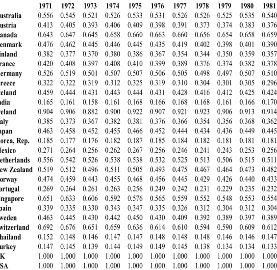
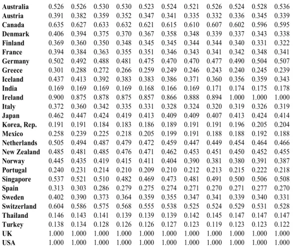
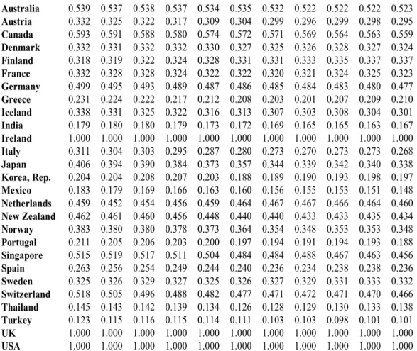
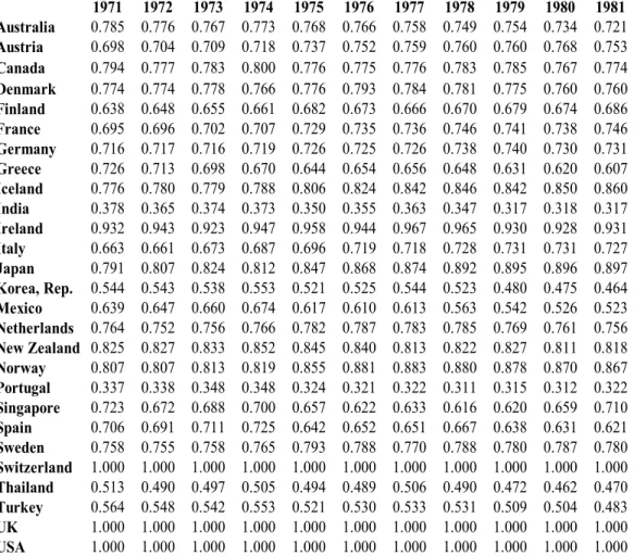
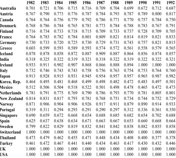
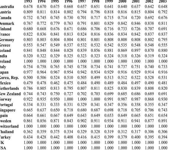
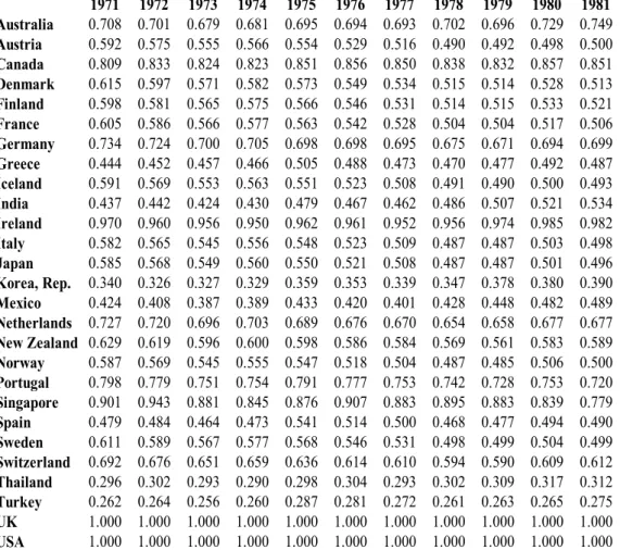
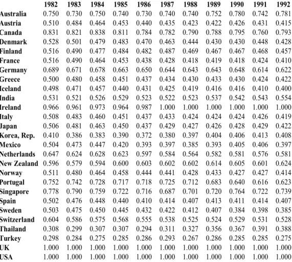
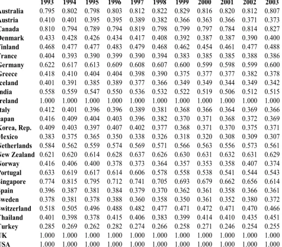
using General Algebraic Modeling System (GAMS) computer program. This procedure is repeated for each year between 1971 and 2003 and 1728 linear programming problems are solved. The ratio of two efficiency numbers computed from two linear programming under the technology that satisfies strongly and weakly disposability of undesirable good gives the index of environmental efficiency for each country. The components of the efficiency index and the resulting environmental efficiency index itself are presented in Table 7.1, Table 7.2 and Table 7.3 respectively.
Table 7.1 and Table 7.2 show the efficiency measures under strong and weak disposability assumptions for pollutants, respectively. Values in these tables show how much inputs and CO2 emissions can be reduced while
simultaneously increasing its outputs and still are in the feasible production sets. To illustrate, in Table 7.1, 0.556 is the value for Australia in the year 1971 under strong disposability assumption of pollutants. This means that the output of Australia can be increased by GDP/0.556 while simultaneously contracting the inputs by Input ×0.556 and CO2 emission by CO2 emission × 0.556 and remain
still in the feasible production set. On the other hand, in Table 7.2, 0.785 is the value for Australia in 1971 under weak disposability of pollutants and shows that the output of Australia can be increased by GDP/0.785 amount while simultaneously contracting the inputs by Input×0.785 and CO2 emission by CO2
emission×0.785 and remain still in the feasible production set.
The values in Table 7.3 are the ratios of corresponding values in Table 7.1 and Table 7.2 and they measure the opportunity cost due to the
transformation of the desirable output in order to reduce the undesirable output. In this table, it is seen that the measure of environmental efficiency takes the value of one for the USA and the UK and less than one for the other countries during the entire sample period. In other words, it can be concluded that the USA and the UK are fully efficient such that there is no opportunity cost for transforming the production process from the one where all outputs are strongly disposable to the one which is characterized by weak disposability of undesirable outputs. For all countries the efficiency measures computed with strong disposability assumption of bad output is lower than the ones computed with weak disposability assumption, in accordance with the theoretical model presented in the previous section. For example, Switzerland is a country that is fully efficient under weak disposability of undesirable good but it is inefficient under strong disposability assumption.
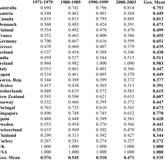
The analysis shows that among all of the 27 countries whereas the UK and the USA have the highest environmental efficiency scores, Mexico, Korea, Thailand and Turkey have the lowest environmental efficiency scores. During the sample periods, Australia, India, Ireland, Korea and Thailand are the only countries that can improve their efficiency scores and most of the other countries such as Iceland, France, Denmark, Mexico and Netherlands reduce their environmental efficiency scores.
The overall picture can be captured by the geometric mean of the environmental efficiency indexes of all countries presented in the following Graph 5 below: It is seen that the environmental efficiency index is deteriorating
through time.16 We compare the geometric mean value of the environmental efficiency index to the total pollution per unit of output as another indicator of environmental quality. In this period both the environmental efficiency index and the pollution per output decline. The decline in the efficiency scores point to the deterioration of the environmental performance whereas pollution per output measures indicate an improvement.
0.45 0.47 0.49 0.51 0.53 0.55 0.57 0.59 0.61 5 5.5 6 6.5 7 7.5 8 1 9 7 1 1 9 7 2 1 9 7 3 1 9 7 4 1 9 7 5 1 9 7 6 1 9 7 7 1 9 7 8 1 9 7 9 1 9 8 0 1 9 8 1 1 9 8 2 1 9 8 3 1 9 8 4 1 9 8 5 1 9 8 6 1 9 8 7 1 9 8 8 1 9 8 9 1 9 9 0 1 9 9 1 1 9 9 2 1 9 9 3 1 9 9 4 1 9 9 5 1 9 9 6 1 9 9 7 1 9 9 8 1 9 9 9 2 0 0 0 2 0 0 1 2 0 0 2 2 0 0 3 Pollution per unit of Output Geometric Mean of Environment Efficiency
Graph 5: Comparison of mean efficiency and total pollution per output
Even though there is no obvious reason for this contradictory result, one may look into the details of the environmental efficiency techniques. Firms' decisions on input use and output mix are taken into consideration in efficiency measures whereas pollution per output isolates only two factors. In this sample of countries we see that production become capital intensive as pollution
16 Table 7.3.1 shows the period averages of the environmental efficiency index for all countries.
intensity measured by pollution per output declined. As illustrated in Graph 6, average output per capital declines and capital per output increases. This might be a reflection of, countries effort to decrease pollution, move to capital intensive technologies. From a perspective of input minimization and output maximization, this change led countries to produce at an environmentally less efficient level.17 Further examination of the properties of the environmental efficiency measurement techniques and the details of the production processes is necessary in order to expose the relationship between alternative environmental performance measures, which is beyond the scope of this study.
0.45 0.47 0.49 0.51 0.53 0.55 0.57 0.59 0.61 2.5 2.7 2.9 3.1 3.3 3.5 3.7 3.9 1 9 7 1 1 9 7 2 1 9 7 3 1 9 7 4 1 9 7 5 1 9 7 6 1 9 7 7 1 9 7 8 1 9 7 9 1 9 8 0 1 9 8 1 1 9 8 2 1 9 8 3 1 9 8 4 1 9 8 5 1 9 8 6 1 9 8 7 1 9 8 8 1 9 8 9 1 9 9 0 1 9 9 1 1 9 9 2 1 9 9 3 1 9 9 4 1 9 9 5 1 9 9 6 1 9 9 7 1 9 9 8 1 9 9 9 2 0 0 0 2 0 0 1 2 0 0 2 2 0 0 3 Output per unit of Capital Geometric Mean of Environment Efficiency
Graph 6: Comparison of mean efficiency and total output per unit of capital
For further analysis of the environmental efficiency values, we group our sample into developed and developing countries in accordance with World Bank
17 Moreover, the capital-labor ratio increases while pollution per unit of capital decreases that supports that claim that the efficiency is declining through time as capital usage is increasing.