Integral equation analysis of an arbitrary-profile
and varying-resistivity cylindrical reflector
illuminated by an E-polarized
complex-source-point beam
Taner Og˘uzer,1,*Ayhan Altintas,2and Alexander I. Nosich3 1
Department of Electrical and Electronics Engineering, Dokuz Eylül University, Buca 35160, Izmir, Turkey
2
Department of Electrical and Electronics Engineering, Bilkent University, 06533 Ankara, Turkey
3Institute of Radio-Physics and Electronics of the National Academy of Sciences of Ukraine, Kharkiv 61085,
Ukraine
*Corresponding author: [email protected]
Received January 9, 2009; revised April 14, 2009; accepted April 17, 2009; posted April 20, 2009 (Doc. ID 106087); published June 9, 2009
A two-dimensional reflector with resistive-type boundary conditions and varying resistivity is considered. The incident wave is a beam emitted by a complex-source-point feed simulating an aperture source. The problem is formulated as an electromagnetic time-harmonic boundary value problem and cast into the electric field inte-gral equation form. This is a Fredholm second kind equation that can be solved numerically in several ways. We develop a Galerkin projection scheme with entire-domain expansion functions defined on an auxiliary circle and demonstrate its advantage over a conventional moment-method solution in terms of faster convergence. Hence, larger reflectors can be computed with a higher accuracy. The results presented relate to the elliptic, parabolic, and hyperbolic profile reflectors fed by in-focus feeds. They demonstrate that a partially or fully re-sistive parabolic reflector is able to form a sharp main beam of the far-field pattern in the forward half-space; however, partial transparency leads to a drop in the overall directivity of emission due to the leakage of the field to the shadow half-space. This can be avoided if only small parts of the reflector near the edges are made resistive, with resisitivity increasing to the edge. © 2009 Optical Society of America
OCIS codes: 050.1755, 050.1940.
1. INTRODUCTION
Accurate characterization of the scattering of waves by three-dimensional (3-D) and two-dimensional (2-D) im-perfect [i.e., not im-perfectly electric conducting (PEC) but partially transparent or lossy] reflectors and mirrors oc-cupy a remarkable place in the electromagnetics across a wide range of frequencies from the visible to microwaves. Imperfection of materials for reflectors is especially im-portant in optics where even noble metals display finite values of both dielectric permittivity and losses. Also, fre-quently the metals are deposited on flat or curved optical surfaces in the form of very thin and hence penetrable layers [1]. In the microwave range, where the losses are negligible, an improvement of metal reflector perfor-mance can be achieved by making its rim transparent, ab-sorptive, or serrated [2–4] . More recently the weight re-strictions imposed on flight-mission antennas have led to development of inflatable microwave reflectors made of thin metallized films [5]. Therefore the scattering and beam forming by a thin penetrable reflector made of di-electric or thinner-than-skin-depth metal is an interest-ing research problem havinterest-ing important applications in optical and microwave imaging systems and antennas.
Today, full-wave modeling of optical and quasioptical reflectors using common finite-difference time-domain (FDTD) codes is not realistic because of the huge size of discrete models and correspondingly huge computation
time. Singular integral equation (SIE) based algorithms are more economic as they discretize only the surface or contour of the reflector. They also satisfy the radiation condition in the explicit manner that is impossible with FDTD codes. The most well-known way of SIE discretiza-tion is the method of moments (MoM) with local or global basis and testing functions [6–9]. Closer inspection, how-ever, shows that within reasonable computation time MoM can be applied only to small- and medium-size re-flectors (roughly up to 10 wavelengths) and provides the accuracy of computing the surface current only within a couple of digits. Numerical examples of this sort can be found in Fig.5of [10]. If a larger geometry or better ac-curacy is a goal, conventional MoM algorithms quickly lead to nonrealistic computer time requirements. More-over, the convergence of the MoM solutions, if applied to the so-called SIE of the first kind that are common for PEC reflectors, is not guaranteed and strongly depends on the implementation.
Alternatives are the high-frequency techniques such as geometrical optics (GO), physical optics (PO), and physi-cal theory of diffraction (PTD), especially for the larger PEC reflectors [11–14]. They have long histories, and the latest sophisticated versions combine PO with Gaussian-beam field decompositions [15–19]. Being powerful engi-neering tools, these asymptotic techniques are still only approximations of the actual solution; all of them fail
near caustics and in the focal domain. PO fails in and near the main beam axis, and GO fails in the complemen-tary domain. They show noticeable errors if a reflector is located near a subreflector, radome, or the Earth’s sur-face. More advanced and mathematically grounded high-frequency analysis could be done with the modified Wiener—Hopf approach [20], but this is still in the future. To overcome these deficiencies, it has been proposed to use SIEs together with the method of analytical regular-ization (MAR) [21]. The MAR can be considered as a judi-cious version of MoM, the difference being in the selection of the expansion functions. With MAR, the original SIE kernel is separated into two parts, namely, the more sgular (usually static) part and the remainder. For in-stance, the former can be the logarithmic part of the 2-D Green’s (i.e., Hankel) function. If the expansion functions are chosen as the orthogonal set of eigenfunctions of the more singular part of the kernel, then their use in the Galerkin-type MoM discretization scheme leads to the analytical inversion of the more singular part of the origi-nal SIE, and the remainder leads to the Fredholm second-kind matrix equation that provides a convergent numeri-cal solution. This technique, combined with the dual-series equations [22] and a wave beam as the incident field, was first applied to a 2-D antenna with reflector shaped as a circularly curved PEC strip [23]. Later it has been extended to the beam-fed 2-D circular PEC reflectors in more complicated near-field environments, including circular dielectric radomes [24] and the flat, imperfect Earth’s surface [25]. Here, the background idea is that these inhomogeneous host media also have analytically derivable Green’s functions which have the same logarith-mic singularities, so that a similar SIE-MAR scheme could be used. Note, however, that a circular arc can ap-proximate only quite shallow parabolic profiles so that deep reflectors and other shapes needed additional ef-forts. In the later work, the SIE-MAR technique has been extended to the 2-D PEC reflectors of noncircular con-tours. As a result, single conical-section-profile reflectors fed with beam sources were computed in the E- and H-polarization cases in [26,10], respectively.
It should be noted that besides MAR, competitive nu-merical solutions of the same SIEs have been recently de-veloped by using a Nystrom-type interpolation technique [27]. One has been successfully used not only in the analysis but also in the synthesis of 2-D PEC reflectors [28] in the E-polarization case.
As for the imperfect 2-D reflectors, a PO treatment has been presented in [29] for the resistive half-plane illumi-nated by a plane wave and, more recently, by a wave beam in [30]. For the curved-screen-like scatterers, a modified-PO study of a 2-D parabolic impedance reflector fed by a line current has been published in [16]. A full-wave numerical analysis has been done with SIE-MAR only for circular-arc 2-D reflectors: a uniform-resistivity one illuminated by a plane wave in [31] and a variable-resistivity one fed by a beam in [32]. The latter analysis confirmed that a noticeable reduction of the penumbral sidelobes could be achieved by loading a PEC reflector with 1—2-wavelength-wide variable-resistivity edges. The spillover lobes are also reduced by a few decibels
com-pared to the PEC case. In fact, such an edge-loaded reflec-tor serves as a simplified model of a serrated reflecreflec-tor.
In the present study, we combine previous 2-D solu-tions of [26,32] and study beam forming by the uniformly and nonuniformly resistive (e.g., edge-loaded) parabolic reflectors fed by beams. Similar to [10,23–28,30,32], we simulate a directive incident beam field by using the complex-source-point (CSP) feed. We also compare perfor-mance of different reflector surface profiles. Here the problem is considered in the E-polarization case; there-fore the SIE obtained is of the Fredholm second kind be-cause of the nonzero jump of the tangential component of the magnetic field across the contour and the logarithmic singularity in the kernel function. Hence, the inversion of this part of SIE is not a necessary procedure. A direct nu-merical solution, if one uses Galerkin projection to a suit-able set of expansion functions, leads to a Fredholm sec-ond kind matrix equation and provides a convergent solution with controlled accuracy.
Thus a MoM-like discrete scheme with local basis func-tions is theoretically sufficient. However, using a set of global expansion functions may provide a more economic numerical solution beyond the limits of conventional MoM. This is important when studying quasioptical-size reflectors. We will develop such an algorithm and analyze basic mechanisms underlying scattering and beam-forming by resistive reflectors of practical shapes.
2. FORMULATION
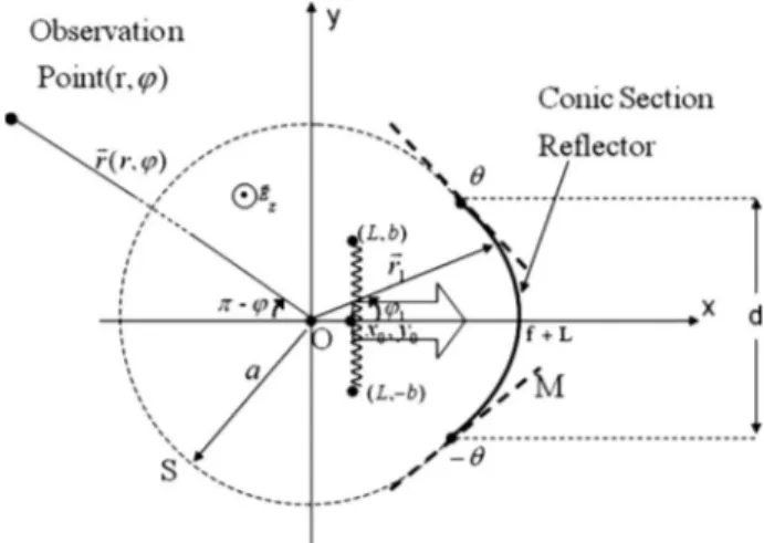
The problem geometry associated with a zero-thickness curved resistive reflector symmetrically illuminated by a directive feed is shown in Fig.1. The 2-D contour of the reflector’s cross-section M can be an elliptic, parabolic, or hyperbolic arc, i.e., an arbitrary conical-section profile. All these curves can be characterized with the same equa-tion, which can be found elsewhere [26]. Here we note only that they differ in the value of the so-called eccen-tricity e so that e⬍1 for an ellipse, e=1 for a parabola, and e⬎1 for a hyperbola.
Fig. 1. Problem geometry for the finite parabolic-profile reflec-tor. Thick dashed straight lines centered at reflector’s edges mark the corresponding tangents. Zigzag line centered at共L,0兲 marks the branch cut associated with the CSP source.
The feed is assumed a CSP source; certain restrictions on its location will appear later due to the singularities of the corresponding field function. In computations, the feed will be placed in the geometrical focus of the reflec-tor, as shown in Fig.1. When building the solution, the open arc of the reflector contour M will be completed to the closed contour C with a circular arc S of a certain ra-dius a. Therefore we will use polar coordinates共r,兲 with the origin at this circle’s center, shifted from the focus of reflector by the distance L.
The rigorous formulation of the considered boundary value problem can be stated in terms of the Helmholtz equation of M, the Sommerfeld radiation condition far from the reflector and source, the resistive boundary con-dition on M, and an edge concon-dition such that the field en-ergy is limited in any finite domain around the reflector edge. Collectively, these conditions guarantee the unique-ness of the problem solution [33].
The resistive boundary condition is a well-established model of a thin penetrable material sheet (see, for in-stance, [34,35]). It can be written as the following pair of equations:
关EជT+共rជ兲 + EជT−共rជ兲兴 = 2R共rជ兲nជ共rជ兲 ⫻ 关HជT+共rជ兲 − HជT−共rជ兲兴,
EជT+共rជ兲 = EជT−共rជ兲, rជ = 共r,兲 苸 M, 共1兲
where Eជ and Hជ are electric and magnetic field functions, respectively; the coefficient R is called resistivity, sub-script T indicates the tangential field, the supersub-scripts “⫺” and “⫹” relate to the front and rear faces of the re-flector, respectively; and the unit normal vector nជ is di-rected from the “⫺” to the “⫹” face. Condition(1)enables one to exclude from consideration the field inside the ma-terial sheet.
The resistivity R in Eq.(1)can be complex-valued and position-dependent on M. The two most frequently met examples of resistive surfaces are a thin dielectric sheet of thickness h and relative permittivity εrand a metal sheet
with thinner-than-skin-depth thickness h and electron conductivity . They are characterized by the following expressions, respectively [34,35]: Rdiel= iZ0 kh共εr− 1兲 , Rmetal= 1 h, 共2兲
where Z0 is the free space impedance, and k is the
free-space wavenumber. Further note that a complex or real-valued R such as Rmetalin(2)corresponds to a lossy sheet,
and a purely imaginary R such as Rdielwith a real εr
cor-responds to the lossless case.
The incident electric field will be taken as the beam-like field generated by the CSP,
Ezin共rជ兲 = H0共1兲共k兩rជ − rជs兩兲, 共3兲
where the complex-valued source point position is given as
rជs=共x0+ ib cos,y0+ ib sin兲. 共4兲
Note that function (3) has two branch points, which should be connected with a branch cut [10,11,23–28]; it also has maximum magnitude along only one direction,
=. Near the cut, function(3)is well approximated by a “one-side” Gaussian beam propagating in the mentioned direction, while further from the cut it smoothly trans-forms into a cylindrical wave. Therefore parameters b and  are the aperture width and the beam-aiming angle, re-spectively, of the directive aperture source simulated with the aid of CSP.
3. BASIC EQUATIONS
By following the formulation outlined in Section 2, the scattered electric field can be presented as a single-layer potential,
Ezsc共rជ兲 = ikZ0
冕
M
Jz共rជ⬘兲G共rជ,rជ⬘兲dl⬘, rជ⬘苸 M, 共5兲
where the scalar Green’s function is a Hankel function of zero order satisfying the radiation condition, i.e.,
G共,
⬘
兲=共i/4兲H0共1兲共k兩rជ共兲−rជ共⬘
兲兩兲, and the unknownsurface current density has only one component defined as
Jz共rជ⬘兲 = HជT+共rជ⬘兲 − HជT−共rជ⬘兲. 共6兲
Then, by imposing the boundary conditions given in Eq.(1), the electric-field integral equation can be derived as
R共rជ兲Jz共rជ兲 − ikZ0
冕
M
Jz共rជ⬘兲G共rជ,rជ⬘兲dl⬘= Ezin共rជ兲, rជ,rជ⬘苸 M.
共7兲 Note that if the resistivity R is not identically zero, then Eq.(7)is a so-called second-kind equation; it is also a Fredholm integral equation (IE), because its kernel has only logarithmic, i.e., integrable, singularity [33]. If, how-ever, R = 0, the PEC counterpart of Eq.(7)is the first-kind equation. Note that Eq.(7)does not permit a continuous transition to the static case of a PEC reflector 共k=0,R = 0兲.
The Fredholm second-kind nature of Eq.(7) suggests that any usual discretization scheme of the order N ap-plied to build a numerical solution to Eq. (7) is conver-gent, i.e., limN→⬁共Jz共N兲− Jz兲=0 [this is unlike the first-kind
PEC counterpart of Eq.(7)]. For instance, this can be a conventional method-of-moments (MoM) discretization with the pulse basis and delta testing functions. Thus, the resistivity R plays the role of regularization parameter; if it is purely imaginary or purely real-valued, adding such a term coincides with regularization in the sense of Lavrentyev [36] or Bakushinsky [37], respectively. Still the convergence of the MoM algorithms is usually not rapid enough to enable the computation of electrically large reflectors with high accuracy. Therefore we develop here a different numerical solution.
Assume that the curve M can be characterized with the aid of the parametric equations x = x共兲, y=y共兲, 0艋兩兩 ⬍ in terms of the polar angle . This puts certain re-strictions on M, which must be convex or at least star-shape. For example, if M is a parabolic arc then r共兲 = L /共cos−cot 1sin兲, where the angle 1 satisfies a
transcendental equation as f sin1= tan关f cos 1
+ Lcos2共
1/ 2兲兴. Then, because of the field continuity
across the virtual arc S, we extend the surface-current density function Jzwith zero value to S and denote it now
as J˜z. This results in the following set of two equations
valid on the complementary parts of the unit circle, 苸关0,2兴: R共兲J˜z共兲 − ikaZ0
冕
0 2 J ˜ z共⬘兲G共,⬘兲l共⬘兲d⬘= Ezin共兲, 0艋 兩兩 ⬍ , 共8兲 J ˜ z共兲 = 0, ⬍ 兩兩 艋 , 共9兲where l共兲=a−1兵关x共兲/兴2+关y共兲/兴2其1/2stands for the
Jacobian normalized to a (see below on the choice of a),
R共兲=R0共兲Z0, and R0共兲 is the normalized
position-dependent resistivity of the curved reflector (for instance, as given below for the edge-loaded case).
To discretize the set of Eqs. (8) and (9), we make a Galerkin projection on the set of entire-domain expansion functions, which are the trigonometric polynomials 兵eim其
m=−⬁
+⬁ . Here, it is convenient to introduce the
un-known expansion coefficients,兵xn其n=−+⬁ ⬁, of the product of
the surface current density function with the Jacobian in the following manner:
X共兲 = J˜z共兲l共兲 = 2 iZ0n=−
兺
⬁ ⬁ 共兩n兩 + 1兲1/2x nein, 共10兲where the factor in the brackets will be justified later (see also [31,32]). In terms of the same functions, the incident field on C = M艛S can be expanded as
Ezinc共兲 =
兺
n=−⬁⬁
bnein, 共11兲
where, in the case of CSP excitation, the coefficients are found as bn= 1 2
冕
0 2 H0共1兲共k兩rជ共兲 − rជs兩兲e−ind, rជ 苸 C. 共12兲The kernel function in (8), which is the Green‘s func-tion, can also be expanded into a double Fourier series; however for an arbitrary arc M the coefficients have to be found numerically. To make their computation more eco-nomic, we add to and subtract from G a similar function given at the full circle of the same radius a as the auxil-iary circular arc S, i.e., H0共1兲关2ka sin共兩−
⬘
兩/2兲兴. There-fore a new function is defined as follows (note that we have used such decomposition earlier in [25] when study-ing a PEC reflector):H共,⬘兲 = H0共1兲共k兩rជ共兲 − rជ⬘共⬘兲兩兲 − H0共1兲关2ka sin共兩 − ⬘兩/2兲兴.
共13兲 The corresponding series representation is
H共,⬘兲 =
兺
m,n=−⬁ ⬁
hnmeineim⬘. 共14兲
Note that this difference function turns to zero at the circular arc S and is not singular if
⬘
→. Further, if the radius of S is chosen in such a way that at the junction points = ±, the curvatures of M and S are matched, then the function H共,⬘
兲 and its first derivatives with respect to and ⬘
are continuous functions on the wholeC. Furthermore the second derivative of H共,
⬘
兲, i.e.,2H共,
⬘
兲/⬘
, has only logarithmic singularity as ⬘
→. Hence, it is not continuous but belongs to L2共C兲,and therefore the Fourier series coefficients hnm decay
rapidly enough (see also [10,26]) to provide that
兺
m,n=−⬁ ⬁
m2n2兩hnm兩2⬍ ⬁. 共15兲
Thus, on performing the Galerkin projection of dual Eqs.(8)and(9)on the trigonometric polynomials, we ob-tain the following dual-series equations:
兺
n=−⬁ ⬁ 共兩n兩 + 1兲1/2x nein = −kal共兲 2R0共兲n=−兺
⬁ ⬁冋
共兩n兩 + 1兲1/2x nJn共ka兲Hn共1兲共ka兲 +兺
p=−⬁ ⬁ hn,−p共兩p兩 + 1兲1/2xp册
ein +i 2 l共兲 R0共兲n=−兺
⬁ ⬁ bnein, 兩兩 ⬍ , 共16兲兺
n=−⬁ ⬁ 共兩n兩 + 1兲1/2x nein= 0, ⬍ 兩兩 艋 . 共17兲Note that the right-hand parts of Eqs.(16)and(17)are two Fourier expansions of the same function of on two complementary arcs of the whole unit circle. Therefore we can use discrete Fourier transform to invert the left-hand parts of Eqs.(16)and(17)and obtain an infinite set of lin-ear algebraic equations for determining the unknowns,
xm+
兺
n=−⬁ ⬁ Amnxn= Bm, m = 0, ± 1, ± 2, . . . , 共18兲 where Amn= ka 2冉
兩n兩 + 1 兩m兩 + 1冊
1/2冋
Jn共ka兲Hn共1兲共ka兲Qnm +兺
p=−⬁ ⬁ hn,−pQpm册
, 共19兲 Bm= i 2共兩m兩 + 1兲1/2兺
s=−⬁ ⬁ bsQsm, 共20兲and the coefficients Qnmare defined as
Qnm= 1 2
冕
− l共兲 R0共兲 ei共n−m兲d. 共21兲The coefficients Qnm decay as O共兩n−m兩−1+␣兲, where 0
艋␣⬍1 (␣=0 for e=0), if the indices get larger. Together with property(15)and large-index asymptotics for cylin-drical functions, this enables one to prove that 兺m,n=−+⬁ ⬁兩Amn兩2⬍⬁. By similar treatment one can find that
兺m=−+⬁ ⬁兩Bm兩2⬍⬁, provided that the branch cut associated
with the CSP aperture does not cross the reflector contour
M.
Now it is clear that the term共兩n兩+1兲1/2introduced “in
advance” in expansion(10)makes the decay of Amn
sym-metric with respect to m→⬁ and n→⬁. As a result, if the above requirements for the configuration of the reflector and feed are satisfied, the resultant infinite-matrix Eq.
(16)is a Fredholm second-kind and has a unique solution 兵xn其n=−+⬁ ⬁ in the class of numerical sequences l2 (i.e.,
兺n=−+⬁ ⬁兩xn兩2⬍⬁). As is known, if such a matrix equation is
truncated and the truncation order, say Ntr, gets larger,
the approximate solution error reduces to zero—see, for instance, the review [21] for details.
Further we will study the far-field characteristics of a resistive reflector illuminated by the CSP feed. Therefore we need a formula linking the far field and the unknown coefficients; that is,
Ez共rជ兲 = 关⌽in共兲 + ⌽sc共兲兴共2/ikr兲1/2eikr, 共22兲
where
⌽in共兲 = e−ikr0cos共−0兲ekb cos共−兲,
⌽sc共兲 = 1 2n=−
兺
⬁ ⬁ x n 共兩n兩 + 1兲1/2冕
− ein⬘−ikr⬘共⬘兲cos共−⬘兲d⬘. 共23兲 The characterization of reflectors is usually done via evaluation of their directivities. In our case, the reflector antenna main beam looks in the direction=, which we will refer to as the forward direction. Then the forward di-rectivity is (see [23] and references therein)Dforw= lim r→⬁
r兩Ez共r,兲H*共r,兲兩2
Prad
, 共24兲
where the denominator is the total power radiated by the CSP feed in the presence of the reflector, averaged over all directions, i.e., Prad= 1 kZ0
冕
0 2 兩⌽in共兲 + ⌽sc共兲兩2d. 共25兲Note that the directivity can also be derived via the far-field scattering pattern,
Dforw=
2兩⌽in共兲 + ⌽sc共兲兩2
kZ0Prad
. 共26兲
As the resistive reflector is partially transparent, we will also compute the backward directivity Dback. This
quantity is similar to(24)and(26), but with=0 instead of.
4. NUMERICAL RESULTS
In the computations, we assume that the CSP feed is in the geometrical focus (x0= L, y0= 0) and illuminates the
reflector in symmetric manner共=0兲. To calculate the ex-pansion coefficients of smooth functions, bmand hmn, we
apply the fast Fourier transform (FFT) and double FFT (DFFT), respectively. Here, the order of FFT and DFFT must be kept sufficiently high to provide a superior accu-racy of filling in the matrix with respect to the matrix truncation error; therefore we have used 2048-point共210兲
transforms. This enables us to examine the convergence of our numerical solution and compare it with that of a conventional MoM algorithm, within at least four digits in the near-field characteristics. The accuracy, for in-stance, of the current density coefficients, is evaluated by computing the error in the sense of the maximum norm as
⌬cur共N兲 =
max兩xnN− xnN+1兩
max兩xnN兩
, 共27兲
where xnN is the coefficient found after solving Eq. (16)
truncated to the order N. Here we would like to empha-size that the use of the Euclidian norm as in [20] leads to the same conclusions.
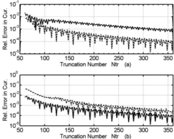
Figure2presents the relative errors in the current den-sity coefficients for several lossy resistivity values of the uniformly resistive reflectors. The curves show the ex-pected convergence and demonstrate that its rate de-pends on the resistivity magnitude: the larger the兩R兩/Z0,
the faster the decrease in error. Generally, our analysis of convergence suggests the following convenient empirical rule: For guaranteed 3-digit accuracy in the current, take the truncation number as N共3兲艌ka/R1/2+ 10.
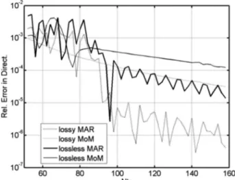
In Figure3, we compare the errors in the computation of the far-field characteristic, the forward directivity ver-sus the matrix truncation number, after the formula
Fig. 2. Relative error in the surface current density versus the matrix truncation number Ntrfor the uniformly resistive lossy reflectors with e = 1 (parabola) and kb = 3. (a) Solid curve is for
R = 0.2Z0and dashed curve is for R = Z0, with other parameters
being d = 20 and f/d=0.5. (b) Solid curve is for d=20 (here, the radius of the auxiliary circle is a = 22.35 and its center’s shift is
L = 12.49) and dashed curve is for d=40 (here, a=44.71 and L = 25.0), with other parameters being f/d=0.5 and R=Z0.
⌬dir共N兲 =
兩DforwN − DforwN+1兩
兩DforwN 兩
. 共28兲
The curves in Fig.3correspond to the numerical solu-tions obtained with conventional MoM algorithm using pulse basis and delta testing functions applied to IE (7)
(thick curves) and our algorithm (thin curves). They dem-onstrate that our solution outperforms MoM approxi-mately by an order in terms of the matrix size necessary for the fixed accuracy. Furthemore, as expected, the accu-racy of determining the far field is an order of magnitude better than that of the near field or surface current.
The normalized radiation patterns of the uniformly re-sistive parabolic reflectors with different lossy and loss-less resistivities are given in Fig.4. These results agree well with the data given in [32] for the circular resistive reflectors. In subfigure (a), one can see how taking the re-flector twice larger makes the main beam twice narrower; this also lowers the sidelobes, but only in the forward halfspace. In subfigure (b), the effect of larger resistivity of the uniformly resistive reflector is seen in the increased and uniform leakage through it. From subfigure (c), the role of the edge taper becomes clear: a less directive inci-dent beam leads to increased sidelobes, but does not dis-tort the forward- and backward-field amplitudes.
The curves in Fig.5show the change in the forward di-rectivity of a uniformly resistive parabolic reflector when its focal distance f / d varies while the aperture size d is fixed. As the in-focus CSP source here is also fixed 共kb = const兲, the reason for such change in Dforwis the
varia-tion of the edge illuminavaria-tion. Examinavaria-tion of the curves leads to the conclusion that the optimal edge illumina-tion, calculated as 20 log关Ezin共edge兲/Ezin共center兲兴, is close to −10 dB, and directivity varies little if it is between −8 and −15 dB.
In Fig.6, we compare the forward and backward direc-tivities of several differently sized all-resistive parabolic reflectors as a function of the absolute value of the lossy and lossless resistivity. Here, the backward directivity is the same as for Eq.(26)but in the direction=0. An in-teresting observation is that if the uniform resistivity of a 10- parabolic reflector is R=1.5Z0, the forward and
back-ward directivities are equal.
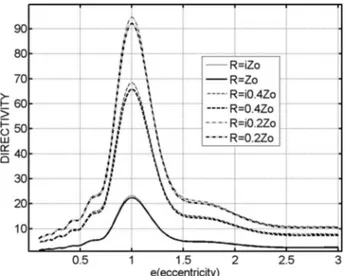
In Fig.7, the forward directivity versus the contour ec-centricity (see Eq.(1)of [25]) of the reflector profile is plot-ted for the different resistivity R values of the uniformly resistive reflectors. For each different R value the maxi-mum directivity occurs at e = 1, i.e., in the case of a pa-rabola, and directivity increases if the surface becomes less transparent. Note that the lossy and lossless cases present not much difference in the D versus e plots.
Fig. 3. Relative error in the far-field directivity versus the ma-trix truncation number Ntrcomputed with MoM and our method
for the uniformly resistive lossy (R is real-valued) and lossless (R is imaginary-valued) parabolic reflectors with d = 10, f/d=0.4,
kb = 3, and兩R兩=0.5Z0. Note that in this case the radius of the aux-iliary circle is a = 9.43 and L=5.56.
Fig. 4. Normalized radiation patterns for the uniformly resis-tive parabolic reflectors illuminated by in-focus CSPs. (a) Solid curve is for d = 20 and dashed curve is for d=40, with other pa-rameters being f / d = 0.5, R = 0.1Z0, and kb = 3. (b) Solid curve is for R = Z0and dashed curve is for R = 0.1Z0, other parameters
be-ing d = 40, f/d=0.5 and kb=3. (c) Solid, dotted and dashed curves are for the CSP sources having kb = 1, 3, and 5, respec-tively. Other parameters are d = 40, f/d=0.5 and R=0.1Z0. As
the lossless reflector patterns are very close to the lossy ones of the same兩R兩, they are not plotted here.
Fig. 5. Directivity as a function of the relative focal distancef / d for three values of parabolic aperture dimensions, d = 15, 20, and 25 plotted as solid, dashed, and dashed—dotted curves, re-spectively. Here, heavy curves are for the uniformly resistive lossless reflector case共R=i0.5Z0兲, light ones are for the lossy case
Finally we have studied the previously reported reduc-tion of the side lobes of the far-field radiareduc-tion pattern for a parabolic reflector by means of varying resistive edge loading. Here, we assumed that the angular size of the re-flector corresponded to 兩兩⬍, and the resistivity as a function of the angular coordinate was a small constant value R共兲=AZ0if兩兩艋1⬍. However starting from 兩兩
=1, it was assumed to grow linearly up to the edge as
R共兲=Z0关A−B1+共B−A兲兩兩兴共−1兲−1 if 1艌兩兩艌, and
reach the value of R = BZ0at the reflector edges. This kind
of study had been earlier performed in [32] for the circular-arc profile simulating a shallow parabolic con-tour, while here it is done for the truly parabolic profile case.
In Figure8, the normalized radiation patterns are com-pared for three types of reflectors: (i) PEC, (ii) “nearly-PEC,” i.e., uniformly resistive with R = 0.01Z0, and (iii)
edge-loaded nearly-PEC as explained above, where we took A = 0.01 and B = 1. One can see that the nearly-PEC case pattern follows the PEC one in the forward half-space but shows some 5 dB higher lobes in the backward half-space, because of partial transparency. The pattern for the edge-loaded reflector (red curve online) follows the nearly-PEC in the backward half-space; however its pen-umbral side lobes are smaller by some 5 dB than for the PEC and nearly-PEC reflectors. This leads to the higher values of the forward directivity for the reflector antenna with resistive edge loading: Dforw= 215.8 and 216.1 in the
edge-loaded lossy and lossless cases, respectively, while it is 208.3 and 207.1 in the case of corresponding nearly-PEC uniformly resistive reflectors.
5. CONCLUSION
We have presented an integral-equation based analysis of arbitrary-profile 2-D reflectors with resistive-surface boundary conditions and illuminated with the E-polarized complex-source-point beams. The problem is discretized using the trigonometric polynomials as global expansion functions introduced on the entire unit circle. This leads to a dual series equation that is partially inverted with the aid of an inverse discrete Fourier transform. The re-sulting infinite-matrix equation is of the Fredholm second kind and exhibits enhanced convergence when truncated and solved numerically. Based on this numerical solution, the normalized far-field patterns and dependences of the pattern directivity on the reflector resistivity and other parameters have been computed. They demonstrate, among other effects, a chance to decrease the edge scat-tering of a parabolic reflector by using varying-resistivity edge loading.
ACKNOWLEDGMENTS
This work was supported by the Turkish National Council for Science and Technology and the National Academy of Sciences of Ukraine via exchange project EEAG-106E209.
Fig. 6. Directivities as a function of absolute value of uniform resistivity for three reflectors with d = 10, 20, and 30, plotted as solid, dashed, and dashed—dotted curves, respectively (lossy and lossless reflector case results are not distinguishable). Heavy curves are for the forward directivity and light curves are for the backward directivity.
Fig. 7. Forward directivity versus the eccentricity of the conical-section-profile reflectors for different R values in lossy and loss-less uniform-resistivity cases. The other parameters are d = 20,
f / d = 0.5, and kb = 3.
Fig. 8. Normalized radiation patterns for the PEC, uniformly resistive “nearly PEC,” and edge-loaded parabolic reflector cases. (a) Lossy and (b) lossless reflector cases, other parameters being
d = 40, f/d=0.5, and kb=3. Also in both figures (a) and (b) the
solid curve is the constant resisitivity case, the bold solid curve is the variable resisitivity case, and the dotted curve is the PEC case.
REFERENCES
1. J. M. Bendickson, E. M. Glytsis, and T. K. Gaylord, “Metallic surface-relief on-axis and off-axis focusing diffractive cylindrical mirrors,” J. Opt. Soc. Am. A 16, 113–130 (1999).
2. H. Yokoi and H. Fukumuru, “Low sidelobes of paraboloidal antennas with microwave absorbers,” Electron. Commun. Jpn. 54-B, 34–49 (1971).
3. O. Bucci and G. Franceschetti, “Rim loaded reflector antennas,” IEEE Trans. Antennas Propag. 28, 297–304 (1980).
4. O. Bucci, G. Di Massa, and C. Savarese, “Control of reflector antennas performance by rim loading,” IEEE Trans. Antennas Propag. 29, 773–779 (1981).
5. E. G. Njoku, Y. Rahmat-Samii, J. Sercel, W. J. Wilson, and M. Moghaddam, “Evaluation of an inflatable antenna concept for microwave sensing of soil moisture and ocean salinity,” IEEE Trans. Geosci. Remote Sens. 37, 63–78 (1999).
6. D. C. Jenn, M. A. Morgan, and R. J. Pogorzelski, “Characteristics of approximate numerical modeling techniques applied to resonance-sized reflectors,” Electromagnetics 15, 41–53 (1995).
7. M. R. Barclay and W. V. T. Rusch, “Moment-method analysis of large, axially symmetric reflector antennas using entire-domain functions,” IEEE Trans. Antennas Propag. 39, 491–496 (1991).
8. B. Philips, M. Philippakis, G. Y. Philippou, and D. J. Brain, “Study of modeling methods for large reflector antennas,” ERA Report 96–0902, U.K., ERA Rep. 96–0902 (1996). 9. A. Heldring, J. M. Rius, L. P. Ligthart, and A. Cardama,
“Accurate numerical modeling of the TARA reflector system,” IEEE Trans. Antennas Propag. 52, 1758–1766 (2004).
10. T. Oguzer, A. I. Nosich, A. and Altintas, “Analysis of arbitrary conic section profile cylindrical reflector antenna, H-polarization case,” IEEE Trans. Antennas Propag. 52, 3156–3162 (2004).
11. F. J. V. Hasselmann and L. B. Felsen, “Asymptotic analysis of parabolic reflector antennas,” IEEE Trans. Antennas Propag. 30, 677–685 (1982).
12. G. A. Suedan and E. V. Jull, “Beam diffraction by planar and parabolic reflectors,” IEEE Trans. Antennas Propag.
39, 521–527 (1991).
13. M. Martinez-Burdalo, A. Martin, and R. Villar, “Uniform PO and PTD solution for calculating plane wave backscattering from a finite cylindrical shell of arbitrary cross section,” IEEE Trans. Antennas Propag. 41,
1336–1339 (1993).
14. H. Anastassiu and P. Pathak, “High-frequency analysis of Gaussian beam scattering by a two-dimensional parabolic contour of finite width,” Radio Sci. 30, 493–503 (1995). 15. U. Yalcin, “Scattering from a cylindrical reflector: modified
theory of physical optics solution,” J. Opt. Soc. Am. A 24, 502–506 (2007).
16. Y. Z. Umul, “Scattering of a line source by a cylindrical parabolic impedance surface,” J. Opt. Soc. Am. A 25, 1652–1659 (2008).
17. H.-T. Chou, P. H. Pathak, and R. J. Burkholder, “Application of Gaussian-ray basis functions for the rapid analysis of electromagnetic radiation from reflector antennas,” Proc. Inst. Electr. Eng. 150, 177–183 (2003). 18. C. Rieckmann, “Novel modular approach based on
Gaussian beam diffraction for analysing quasi-optical multireflector antennas,” Proc. Inst. Elect. Eng. Microwaves 149, 160–167 (2002).
19. A. Tzoulis and T. F. Eibert, “A hybrid FEBI-MLFMM-UTD method for numerical solutions of electromagnetic
problems including arbitrarily shaped and electrically large objects,” IEEE Trans. Antennas Propag. 53, 3358–3366 (2005).
20. M. Idemen and A. Büyükaksoy, “High frequency surface currents induced on a perfectly conducting cylindrical reflector,” IEEE Trans. Antennas Propag. 32, 501–507 (1984).
21. A. I. Nosich, “MAR in the wave-scattering and eigenvalue problems: foundations and review of solutions,” IEEE Antennas Propag. Mag. 42, 34–49 (1999).
22. A. I. Nosich, “Green’s function—dual series approach in wave scattering from combined resonant scatterers,” in M. Hashimoto, M. Idemen and O. A. Tretyakov, eds.,
Analytical and Numerical Methods in Electromagnetic Wave Theory (Tokyo: Science House, 1993), pp. 419–469.
23. T. Og˘uzer, A. Altintas, and A. I. Nosich,“Accurate simulation of reflector antennas by the complex source— dual series approach,” IEEE Trans. Antennas Propag. 43, 793–802 (1995).
24. V. B. Yurchenko, A. Altintas, and A. I. Nosich, “Numerical optimization of a cylindrical reflector-in-radome antenna system,” IEEE Trans. Antennas Propag. 47, 668–673 (1999).
25. S. V. Boriskina, A. I. Nosich, A. and Altintas, “Effect of the imperfect flat earth on the vertically-polarized radiation of a cylindrical reflector antenna,” IEEE Trans. Antennas Propag. 48, 285–292 (2000).
26. T. Og˘uzer, A. I. Nosich, and A. Altintas, “E-polarized beam scattering by an open cylindrical PEC strip having arbitrary conical-section profile,” Microwave Opt. Technol. Lett. 31, 480–484 (2001).
27. A. A. Nosich and Y. V. Gandel, “Numerical analysis of quasioptical multi-reflector antennas in 2-D with the method of discrete singularities: E-wave case,” IEEE Trans. Antennas Propag. 57, 399–406 (2007).
28. A. A. Nosich, Y. V. Gandel, T. Magath, and A. Altintas, “Numerical analysis and synthesis of 2-D quasioptical reflectors and beam waveguides based on an integral-equation approach with Nystrom’s discretization,” J. Opt. Soc. Am. A 24, 2831–2836 (2007).
29. T. B. A. Senior, “Some problems involving imperfect half-planes,” in P. L. E. Uslenghi, ed., Electromagnetic Scattering (Academic, 1978), pp. 185–219.
30. Y. Z. Umul, “Scattering of a Gaussian beam by an impedance half-plane,” J. Opt. Soc. Am. A 24, 3159–3167 (2007).
31. A. I. Nosich, Y. Okuno, and T. Shiraishi, “Scattering and absorption of E and H-polarized plane waves by a circularly curved resistive strip,” Radio Sci. 31, 1733–1742 (1996). 32. A. I. Nosich, V. B. Yurchenko, and A. Altintas, “Numerically
exact analysis of a two-dimensional variable-resistivity reflector fed by a complex point source,” IEEE Trans. Antennas Propag. 45, 1592–1601 (1997).
33. D. Colton and R. Kress, Integral Equation Method in
Scattering Theory (Wiley, 1983).
34. E. Bleszynski, M. Bleszynski, and T. Jaroszewicz, “Surface-integral equations for electromagnetic scattering from impenetrable and penetrable sheets,” IEEE Trans. Antennas Propag. 35, 14–25 (1993).
35. G. Bouchitte and R. Petit, “On the concepts of a perfectly conducting material and of a perfectly conducting and infinitely thin screen,” Radio Sci. 24, 13–26 (1989). 36. M. M. Lavrentyev, V. G. Romanov, and S. P. Shishatskii,
Ill-Posed Problems in Analysis and Mathematical Physics
(Moscow, Nauka Publ., 1980) (in Russian).
37. A. B. Bakushinsky, “About one numerical method of solving the Fredholm first-kind integral equations,” Comput. Math. Math. Phys. 5, 744–749 (1965).