Performance evaluation of track association and maintenance for a MFPAR with doppler velocity measurements

https://www.researchgate.net/publication/270083451

Performance evaluation of track

association and maintenance for

a MFPAR with Doppler velocity

measurements

Article in Progress In Electromagnetics Research · January 2010 DOI: 10.2528/PIER10070801 CITATIONS

10

READS

21

4 authors, including: Some of the authors of this publication are also working on these related projects: Bayesian RFS Estimators

View project Unbiased and No restriction on Pd

View project F. Arikan Hacettepe University 111 PUBLICATIONS 638 CITATIONS SEE PROFILE Orhan Arikan Bilkent University 162 PUBLICATIONS 2,060 CITATIONS SEE PROFILE

All content following this page was uploaded by F. Arikan on 12 November 2016. The user has requested enhancement of the downloaded file.

PERFORMANCE EVALUATION OF TRACK ASSOCI-ATION AND MAINTENANCE FOR A MFPAR WITH DOPPLER VELOCITY MEASUREMENTS

F. Kural

Meteksan Defence Ind. Inc. Bilkent Cyberpark

Bilkent University Ankara, Turkey F. Arıkan

Department of Electrical and Electronic Engineering Hacettepe University

Beytepe, Ankara, Turkey O. Arıkan

Department of Electrical and Electronic Engineering Bilkent University

Bilkent, Ankara, Turkey M. Efe

Department of Electronic Engineering Ankara University

Tando˘gan, Ankara, Turkey

Abstract—This study investigates the effects of incorporating Doppler velocity measurements directly into track association and maintenance parts for single and multiple target tracking unit in a multi function phased array radar (MFPAR). Since Doppler velocity is the major discriminant of clutter from a desired target, the measurement set has been expanded from range, azimuth and elevation angles to include Doppler velocity measurements. We have developed data association and maintenance part of a well known tracking method, Interacting Multiple Model Probabilistic Data Association

Received 8 July 2010, Accepted 12 September 2010, Scheduled 22 September 2010 Corresponding author: F. Kural (fkural@meteksansavunma.com.tr).

Filter (IMMPDAF), with the Doppler velocity measurements and demonstrated the performance improvement through simulations in terms of track update interval, track maintenance rate, RMS position estimation error, probability of detection and processing time. Since Doppler velocity measurements are employed in track maintenance, non-linear filters are used in the scheme leading to the use of Extended Kalman Filter (EKF) based PDAF. Comprehensive simulations have revealed that using Doppler velocity measurements along with 3D position measurements in heavy clutter conditions lead to an increase in track maintenance rate, track update interval; a decrease in position estimation error, processing time and no considerable effect on the probability of detection. This result is very significant for the efficient use of the limited resources of a multi function phased array radar.

1. INTRODUCTION

The problem of target tracking has been an important issue of signal and data processing for many years and a variety of tracking methods have been recommended in the literature [1–7]. A Multi Function Phased Array Radar (MFPAR) is capable of transmitting and receiving electromagnetic waves electronically with its phase shifters to the directions calculated by the tracker [8] and therefore, it removes the requirement of a mechanically rotating antenna. Performance of the target tracking unit of an MFPAR in complex environments heavily relies on the success of Track Initiation (TI) and Track Association and Maintenance (TAM) algorithms. In an MFPAR system, extracted measurements from the detections are transferred to the target tracking unit with a transfer rate allowed by the MFPAR. The measurements are first fed into the measurement-to-track association (shortly, track association) unit that correlates the measurements with the tracks being already initiated. The measurements which are not correlated with the registered tracks are assumed to have originated from new potential targets and they are directed to the TI unit. The performance of TI has a vital importance for tracking systems. When a TI unit fails to initiate real tracks, the radar may miss potential targets. In the cases where TI unit initiates false tracks, already limited resources of MFPAR are wasted on non-existing targets resulting in the reduction of the number of targets to be tracked. Thus, it is very critical of TI to correctly initiate the real tracks in a required period of time. Furthermore, TI should also suppress the measurements originated from false detections. A statistically successful TI should be able to set its true track initiation probability to an acceptable level while keeping

the false track initiation probability as low as possible [9].

Following the TI process, TAM unit essentially determines the performance of the tracking system. An MFPAR is capable of using an adaptive sampling policy by the agile beam positioning. Especially for multiple target environments with heavy clutter, increasing the duration between two samples of a track, i.e., track update interval, reduces the computational complexity leading to conservation of radar energy for more demanding tasks such as simultaneous tracking of increased number of targets. However, longer track update intervals may also result in an increase in the position estimation errors which will reduce the probability of detection. The most common performance measures of a TAM unit are RMS position estimation error, track maintenance rate, probability of detection, track update

interval and processing time. The major design criteria for a

TAM unit in an MFPAR are to increase the track update interval, track maintenance rate and probability of detection while decreasing estimation error and processing time to allocate the radar resources efficiently. Owing to the beam steering capability of MFPAR systems, track update interval can be modified adaptively. Such a control is essential for efficient allocation of the MFPAR resources. For instance, using high update rates to track a non-maneuvering target is not usually necessary. The expected tracking performance can still be achieved with longer track update intervals for a target that reduces the burden on system resources. Contrarily, utilizing high track update rate for a maneuvering target is very important with regard to the

required tracking performance. Therefore, a TAM algorithm that

is capable of scheduling electromagnetic beams and steering them correctly to the predicted positions of the tracked target is of critical importance.

In order to track targets with complex motion capabilities, Interacting Multiple Model (IMM) algorithm has been proved to be

very effective [1, 2]. However, in the presence of clutter, a track

association utility is necessary to assign corresponding weights to the extracted measurements. Probabilistic Data Association Filter (PDAF) is one of the commonly used method for this purpose [1, 2]. A combination of these two methods, Interacting Multiple Model Probabilistic Data Association Filter (IMMPDAF) structure, will be used in this study as a TAM technique where 3D position measurements are typically used. However, the major discriminant of clutter from the target of interest is Doppler velocity (or range rate) measurement. The incorporation of Doppler velocity measurement in a phased array radar for track initiation and maintenance is described in [9–11]. The use of Doppler velocity measurement to increase ECCM

capability of a generic radar is presented in [12]. A new statistic of accelerations based on the range rate measurement is provided in [13]. The statistic turns out to be a reliable indicator of a maneuver and it is also a good estimator of the acceleration. The new method compares favorably to a two mode IMM and a tracker that switches process noise levels based on the position measurement innovations. In [14], Doppler velocity measurements are utilized in the Multiple Hypothesis Tracker (MHT). The results indicate a reduction in false track rate, confirmation time and computational requirements when the track initiation rate is increased due to more efficient return-to-track association process in TI. In [15], velocity based track discrimination is posed as a detection problem. Some parametric data are presented showing the effects of combining velocity measurements with the usual position measurements in a simple form of target tracking Kalman filter [16]. Also, the effects on steady-state performance and filter gains are shown, as well as the time required for convergence to steady state. An adaptive, non-linear algorithm using both position and radial velocity measurements in a Track-While-Scan (TWS) based radar for targets in a clutter environment is presented in [17]. In [18], a one-point track initiation method is derived for conventional target tracking systems where noisy sensor measurements of both target position and Doppler velocity are available. It is shown that the proposed method will exhibit a much shorter true track confirmation delay than a similar system based on the standard approach. In [19, 20], one-point track initiation and an efficient Doppler data association method are used as a variety of PDAF technique in an active sonar underwater multi-target tracking scenario. A modified joint probabilistic data association (JPDA) algorithm that uses range rate measurements in addition to position measurements using a nonlinear measurement model is given in [21]. In [22], a tracking algorithm using both position and range rate for a target from a phased array radar is presented. The results show that the EKF with the Doppler velocity measurements provides a good performance especially for the target maneuvers. In [23], an IMM estimator consisting of a number of EKF modules is used to cope with target range rate measurements for an airborne early warning

system tracking scenario. In all of the existing methods outlined

above, an important achievement is the improved data initiation and association performance by using the incorporation of Doppler velocity measurements. In this study, we demonstrate the further improvement achieved on the comprehensively defined performance measures of the developed IMMPDAF algorithm by the direct inclusion of Doppler velocity measurements along with 3D position measurements. Since Doppler velocity measurements are employed in track maintenance,

non-linear filters are used in the scheme leading to the use of Extended Kalman Filter (EKF) based PDAF. In order to control the track update interval, a commonly preferred technique is used where the selection of update interval is based on the predicted values of the radar angle innovation standard deviations relative to the radar beamwidth [24].

The outline of the paper is as follows; Section 2 gives a brief description of the widely used TAM scheme, IMMPDAF, and some analytical derivations of developed IMMPDAF with 3D position plus Doppler velocity measurements. In Section 3, the results of computer simulations are provided.

2. TRACK ASSOCIATION AND MAINTENANCE SCHEME

In modern target tracking systems, Kalman filter is a widely used state estimator which gives the optimal minimum mean square error providing that the system is linear; initial state vector and system

disturbances are white Gaussian distributed [1, 25, 26]. It is also

the best estimator in case of non-Gaussian initial state vector and disturbances for linear systems. From the viewpoint of target tracking, process noise matrix in Kalman filter defines a model concerning for the target motion. However, complex targets may obey more than one motion model and some serious problems would arise if only one motion model was used. Therefore, one needs more than one model to better identify the motion characteristics of a target. One way of doing so is to run N-parallel Kalman filters with different process noise matrices. The approach of using multiple Kalman filters run in parallel and at a given time, choosing the output from the best filter to represent the current target state is called multiple model filtering. One of the very efficient implementation of the multiple model approach is the IMM in which the state estimates and the covariance matrices from the multiple models are combined together according to a Markov model for the transition between maneuver states [1, 25, 26]. The discrete time state equation for IMM is given by [1]:

x(t_k) = F(m (t_k) , δ_k−1)x(t_k−1) + G(m (t_k) , δ_k−1)v(t_k) (1)

The corresponding measurement equation derived from (1) is:

z(tk) = H(tk)x(tk) + w(tk) (2)

In (1) and (2), tk is the kth sampling time, m (tk) is the effective

model mj from t(k−1) to tk, mj is the jth model among totally r

possible motion models (m (tk) ∈ mj, j = 1, . . . , r), x(tk), z(tk), v(tk)

noise vectors, respectively. F(m (t_k) , δ_k−1) and G(m (t_k) , δ_k−1) are

the state transition and process noise matrices, both at time t_k,

respectively. The values of the matrices are dependent on both kth sampling time and the time difference between kth and (k − 1)th

sampling times, namely the track update interval, δ_k−1 = t_k− t_k−1,

obtained at (k − 1)th sampling time. The covariance matrices of

measurement and process noise at time tk are independent of each

other and defined as M(tk) and Q (m (tk) , δk−1), respectively. H(tk)

is the measurement matrix at time tk.

During the search function of an MFPAR system, the

measurements extracted from the search region are transferred to the TI unit with an allowable transfer rate of the MFPAR. This period can be constant or varying depending on the requirements. However, in TAM, track update interval can be determined based on an adaptive algorithm according to the maneuver capabilities of the targets under track. The transition between different models of IMM is accommodated with model transition probabilities. These transition probabilities can be updated at each sampling time depending on the current track update interval of the target under track. The chain obtained by updating the model transition probabilities depending on the current update interval is essentially in a class of a semi-Markov chain and it represents the target motion better [27, 28]. In

this case, the model transition probabilities, (pij(δk−1) ∈ Π(δk−1),

(i, j = 1, . . . , r) are defined as [1]:

pij(δk−1)= P {m (t∆ k) = mj |m (tk−1) = mi} (3)

In (3), P {·} is the probability of the event given in the curly

brackets and p_ij(δ_k−1) is the probability of the model j at time t_kgiven

the system was in model i at time t_k−1. For a simpler notation, t_k−1will

be denoted by the index k − 1. The model transition matrix, Π(δ_k−1),

is composed of these probabilities and is given in [1]. Some definitions in IMMPDAF are summarized in Table 1. In the definitions, SVE, SVP, EVSV and CME stand for State Vector Estimate, State Vector Prediction, Expected Value of State Vector and Covariance Matrix Estimate, respectively.

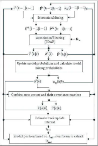
A general flow diagram of the IMMPDAF structure is given

in Fig. 1. In IMMPDAF, interaction/mixing process produces

mixed state vector, ˆx0j_{(k − 1 |k − 1 ), and its covariance matrix,}

ˆ

P0j(k − 1 |k − 1 ), using state vector estimates, ˆxi(k − 1 |k − 1 ),

covariance matrices, Pˆi(k − 1 |k − 1 ), and mixing probabilities,

µ_i|j(k − 1 |k − 1), for each model. The mixed values are then

transferred to the PDAF structure corresponding to each model

Table 1. Summary of some definitions used in IMMPDAF.

(i, j = 1, . . . , r) Model indices

(k, l) Time indices

Zk₌£ _{R1 R2 . . . R} k

¤

Measurement matrix up to kth sampling time Rk=

£

rk;1 rk;2 . . . rk;Nk

¤

Measurement submatrix at kth sampling time rk;s=

£

xk;syk;s zk;s υk;s

¤T _{sth measurement vector at kth sampling time} ˆ x(l |k )∆= Ehx(l) ¯ ¯ ¯Zk i

EVSV at lth sampling time given Zk

ˆ

x(l |k ), l = k SVE given Zk

ˆ

x(l |k ), l > k SVP given Zk

ˆ

xj_d(k |k ) SVE with jth model and dth validated meas. given Zk

ˆ

xi_{(k − 1 |k − 1 ) SVE with ith model given Z}k−1

ˆ

Pi_{(k − 1 |k − 1) CME of state vector with ith model given Z}k−1

ˆ

x0j_{(k − 1 |k − 1) Mixed initial SVE given Z}k−1

ˆ

P0j_{(k − 1 |k − 1) CME of initial mixed state vector given Z}k−1

ˆ

Pi_{(k |k ), and likelihood function, Λ}i_{(k). Using these values, model}

mixing probabilities, µ_i|j(k |k ), and model probabilities, µi_{(k), are}

determined. Then, a final state vector estimate, ˆx (k |k ), its

covariance matrix, ˆP (k |k ), state update interval, tk+1, and state

vector prediction, ˆx (k + 1 |k ), are computed for the target under track

utilizing the previous outputs. Then, an assigned beam of the MFPAR is steered to the predicted position to make an effort to extract possible measurements for the target under track. Details of the IMMPDAF approach can be found in [1, 25, 26]. Following subsection details the target motion models employed in the IMM structure.

2.1. Target Motion Models

In this subsection, target motion models utilized in IMM structure are discussed. In this study, an IMM structure with three models is employed for the accurate representation of the motion characteristics of the target.

2.1.1. Benign Motion Model, m₁

The Benign motion model is also known as white noise acceleration model [1, 25, 26]. It is used to represent the constant velocity regimes of a target. In real life, due to some atmospheric and physical conditions, very small acceleration values may appear. Such acceleration can be characterized by a zero mean Gaussian distributed white noise which is defined as the process noise of the system and it is given by its covariance matrix, called process noise matrix [1, 25, 26]. The values of

standard deviation of process noise for such motion, σ_v1, is generally

chosen between 1 to 5 m/s2 _{[1, 25, 26].}

2.1.2. Maneuver Motion Model, m2

In case of a maneuvering of a target, the standard deviation of process noise can be increased to a fraction of the maximum acceleration

level of the target of interest, a_max, such as σ_v2 = αa_max where

(0.5 < α ≤ 1) [1, 25, 26].

2.1.3. Maneuver Start/Stop Model, m3

Maneuver Start/Stop Model is also known as Wiener process

acceleration model [1, 25, 26]. When a target moves in constant

acceleration, possible fluctuations around this constant acceleration is modeled as a Wiener-type process noise which results in a time-varying acceleration. In this model, the change of acceleration value is

taken as a zero mean Gaussian distributed random variable with the

standard deviation of σ_v3(k) = min (0.5 ˙a_maxδ_k−1, a_max) where ˙a_max is

the assumed maximum jerk value of the target of interest [1, 25, 26]. 2.2. Doppler Velocity Incorporation

In this subsection, Doppler velocity inclusion into the TAM method is outlined. For this reason, first we define the measurement matrix given in (2), where the values of state and measurement vectors are to be predicted. The state prediction vector is a 9-dimensional vector including position, velocity and acceleration values in 3D and defined for jth model and kth sampling time as:

ˆ xj(k |k − 1 ) = h ˆ xj_{(k |k − 1 ) ˆ˙x}j_{(k |k − 1 ) ˆ¨x}j_{(k |k − 1 ) . . .} ˆ yj_{(k |k − 1 ) ˆ˙y}j_{(k |k − 1 ) ˆ¨y}j_{(k |k − 1 ) . . .} ˆ zj_{(k |k − 1 ) ˆ˙z}j_{(k |k − 1 ) ˆ¨z}j_{(k |k − 1 )} i_T 9×1 (4)

where ˆxj_{(k |k − 1 ), ˆy}j_{(k |k − 1 ) and ˆz}j_{(k |k − 1 ) are the position}

pre-dictions; ˆ˙xj(k |k − 1 ), ˆ˙yj(k |k − 1 ), ˆ˙zj(k |k − 1 ) are the velocity

predic-tions and ˆ¨xj(k |k − 1 ), ˆ¨yj(k |k − 1 ), ˆ¨zj(k |k − 1 ) are the acceleration

predictions, all in Cartesian coordinates. The measurement prediction vector in case of the existence of Doppler velocity measurement for jth

model of the system, ˆzj_{(k |k − 1 ), is calculated as:}

ˆzj(k |k−1) =     rj_{(k |k − 1 )} θj(k |k − 1 ) φj_{(k |k − 1 )} ˙rj_{(k |k − 1 )}     =               q ˆ xj_{(k |k − 1 )}2_{+ ˆy}j_{(k |k − 1 )}2_{+ ˆz}j_{(k |k − 1 )}2 tan−1¡_yˆj_{(k |k − 1 )/ˆx}j_{(k |k − 1 )}¢ tan−1 µ ˆ zj_{(k |k−1)/} µq ˆ xj_{(k |k−1)}2_{+ ˆy}j_{(k |k−1)}2 ¶¶  xˆj(k |k−1 )ˆ˙x j (k |k−1)+ ˆyj_{(k |k−1)ˆ˙y}j_{(k |k−1)} +ˆzj_{(k |k − 1 )ˆ˙z}j_{(k |k − 1 )}   q ˆ xj_{(k |k − 1 )}2_{+ ˆy}j_{(k |k − 1 )}2_{+ ˆz}j_{(k |k − 1 )}2               (5)

where rj(k |k − 1 ) is the prediction of range measurement, θj(k |k − 1 )

is the prediction of azimuth angle measurement, φj(k |k − 1 ) is the

prediction of Doppler measurement for jth model at kth sampling time. The measurement vector is a non-linear function of the state vector as shown in (5) leading to the use of an extended Kalman Filter (EKF) based PDAF scheme. Therefore, as stated previously, instead of the measurement matrix, a first degree Taylor series expansion of the measurement equation is employed to obtain the Jacobian of H(k).

The Jacobian of the measurement matrix, HJ_{(k), is defined as:}

HJ(k)=∆ ³ ∇_x(k)(H(k)x(k))T ´_T¯_¯ ¯ ¯ x(k)=ˆxj_{(k|k−1 )} (6) where ∇_x(k)= h ∂ ∂x(k) ∂ ˙x(k)∂ ∂ ¨x(k)∂ . . . ∂

∂y(k) ∂ ˙y(k)∂ ∂ ¨y(k)∂ . . . ∂

∂z(k) ∂ ˙z(k)∂ ∂ ¨z(k)∂

i_T

9×1

(7)

is the gradient operator defined for the 9-dimensional state vector [25].

The gradient value of the vector (H(k)x(k))T is calculated using (7)

as [25]: ³ ∇_x(k)(H(k)x(k))T ´ = h ∂ ∂x(k) ∂ ˙x(k)∂ ∂ ¨x(k)∂ . . . ∂

∂y(k) ∂ ˙y(k)∂ ∂ ¨y(k)∂ . . . ∂ ∂z(k) ∂ ˙z(k)∂ ∂ ¨z(k)∂ i_T 9×1 h (H(k)x(k))T i 1×h (8)

Since the Jacobian matrix is transpose of (8), the Jacobian of the measurement matrix is derived as:

HJ(k) = [ H1(k) H2(k) 0h×3 ]_h×9 (9)

where h = 3 for position only measurements and h = 4 for position

and Doppler velocity measurements. In order to calculate HJ_{(k), the}

submatrices are decomposed as:

where h1(k) =                          ˆ xj_{(k |k − 1 )} rj_{(k |k − 1 )} −ˆyj_{(k |k − 1 )} ˆ xj_{(k |k − 1 )}2_{+ ˆy}j_{(k |k − 1 )}2 −ˆxj_{(k |k − 1 )ˆz}j_{(k |k − 1 )} rj_{(k |k − 1 )}2 q ˆ xj_{(k |k − 1 )}2_{+ ˆy}j_{(k |k − 1 )}2       ˆ˙xj(k |k − 1 ) ³ ˆ zj_{(k |k − 1 )}2_{+ ˆy}j_{(k |k − 1 )}2´ −ˆxj_{(k |k − 1 )} Ã ˆ yj_{(k |k − 1 )ˆ˙y}j_{(k |k − 1 )} +ˆzj_{(k |k − 1 )ˆ˙z}j_{(k |k − 1 )} !       rj(k |k − 1 )3                          (11) h2(k) =                          ˆ yj(k |k − 1 ) rj_{(k |k − 1 )} ˆ xj_{(k |k − 1 )} ˆ xj_{(k |k − 1 )}2_{+ ˆy}j_{(k |k − 1 )}2 − yˆj(k |k − 1 )ˆzj(k |k − 1 ) rj_{(k |k − 1 )}2 q ˆ xj_{(k |k − 1 )}2_{+ ˆy}j_{(k |k − 1 )}2       ˆ˙yj (k |k − 1 ) ³ ˆ zj_{(k |k − 1 )}2_{+ ˆx}j_{(k |k − 1 )}2´ −ˆyj(k |k − 1 ) Ã ˆ xj_{(k |k − 1 )ˆ˙x}j_{(k |k − 1 )} +ˆzj_{(k |k − 1 )ˆ˙z}j_{(k |k − 1 )} !       rj(k |k − 1 )3                          (12)

h3(k)=                        ˆ zj_{(k |k − 1 )} rj_{(k |k − 1 )} 0 q ˆ xj_{(k |k − 1 )}2_{+ ˆy}j_{(k |k − 1 )}2 rj_{(k |k − 1 )}2       ˆ˙zj (k |k − 1 ) ³ ˆ xj_{(k |k − 1 )}2_{+ ˆy}j_{(k |k − 1 )}2´ −ˆzj(k |k − 1 ) Ã ˆ yj_{(k |k − 1 )ˆ˙y}j_{(k |k − 1 )} +ˆxj_{(k |k − 1 )ˆ˙x}j_{(k |k − 1 )} !       rj(k |k − 1 )3                        (13) and H₂(k) =     0 0 0 0 0 0 0 0 0 ˆ xj_{(k|k−1 )} rj_{(k|k−1 )} ˆ yj_{(k|k−1 )} rj_{(k|k−1 )} ˆ zj_{(k|k−1 )} rj_{(k|k−1 )}     (14)

In case of position only measurements, the last row of H1(k)

and H2(k) has to be removed. In this way, the measurement

matrix is defined as a function of the state vector prediction given above for jth model at kth sampling time. After interaction/mixing, association/filtering and model probabilities update, the next step in IMMPDAF structure is to estimate track update interval for the corresponding track for the computation of the state prediction vector. Finally, position predictions are utilized to steer an idle beam of MFPAR to attempt to extract possible measurements for the target under track.

2.3. Estimation of Track Update Interval

In the open literature, a number of efficient track update interval estimators are available [24, 29]. In [29], no clutter is assumed for the estimation of track update interval. The second method in [24] that is widely used for clutter conditions is utilized in this study. In

this method, track update interval, δ_k, is selected from one of the

entries of a constant update interval vector, t. The contents of this vector are application dependent. However, in this study, the values of this vector are chosen in parallel with the benchmark given in [30] as

measurement falls inside the validation region, track update interval is

chosen as δ_k= δmin

k = 0.1 s. The algorithm is given as:

(i) Begin test with the maximum value of vector t;

(ii) Calculate the state vector prediction and substitute it in (6) to

obtain HJ_(k);

(iii) Using HJ_{(k) and covariance matrix of the state vector, calculate}

the covariance matrix of the residual vector using (15) as: ˆ

S (k + 1) = HJ(k + 1) ˆP (k + 1 |k ) HJ(k + 1)T+M (k + 1) (15)

(iv) Choose the diagonal elements related to the corresponding

angles in residual matrix, ˆS (k + 1), namely ˆS (k + 1) (2, 2) and

ˆ

S (k + 1) (3, 3) as test variables;

(v) Compare both test variables to a fraction, η, of the half power

beamwidth values of the MFPAR, ηϕ3 dB;

(vi) If test variable is less than or equal to the calculated threshold, track update interval under test is chosen as the final interval value, else the following track update interval under test is chosen and go to (ii);

(ii) If the test variables do not satisfy the conditions, choose the track

update interval as δk= δkmin= 0.1 s.

2.4. System Performance Measures

In order to obtain the performance of the TAM algorithm for an MFPAR, a comprehensive set of system performance measures are

defined in detail. These performance measures are given in the

following subsections.

2.4.1. Track Update Interval (~)

Track update interval is the time taken to receive a new measurement from the target being tracked. Longer track update intervals with acceptable level of estimation error is preferred for a given target. In

case where the number of Monte-Carlo run is chosen as NMC and the

maximum number of update is limited to N_k for each run, a track

update interval matrix, ~~~, with the size of N_k× N_{M C} is formed using

N_k track updates of cth run of a simulation. The average track update

interval is calculated as:

~ = 1 Nk à NPM C c=1 ytmr(c) ! NXM C c=1 à ytmr(c) Nk X k=1 ~~~(k, c) ! (16)

where y_tmr is provided in the following subsection. 2.4.2. Track Maintenance Rate (ytmr)

Track maintenance rate is defined as the ratio of tracks that are

not dropped. A successful track maintenance unit is expected to

detect different maneuver magnitudes of targets. Therefore, track maintenance rate for a tracker is a very important performance parameter which is related to the number of track drop occurrence within a number of simulations. The track maintenance rate for a single simulation and its average along several simulations are given as: ytmr(c) = ½ 1 hpos(k, c) ≤ 1.5rg, for ∀k 0 otherwise ytmr= _{NM C}1 NPM C c=1 ytmr(c) (17)

where r_g is the value of range gate for tracking function of MFPAR

and h_pos is defined in the next subsection.

2.4.3. RMS Position Estimation Error (hpos)

Position estimation error is the main indicator of how well the tracker models the target motion at a given sampling time and it will directly affect the previously defined performance measures, namely the track update interval as well as the track maintenance rate. RMS position estimation error is calculated as a function of difference between the

state vector estimation at the kth sampling time (k = 1, . . . , Nk) of cth

run (c = 1, . . . , NM C) of a simulation,bˆxc(k), and the true state vector

at the kth sampling time, xt(k), as:

hpos(k, c) = s ¡_b ˆ xc(k) (1) − xt(k) (1) ¢₂ +¡b_xˆ c(k) (4) − xt(k) (4) ¢₂ +¡b_ˆx c(k) (7) − xt(k) (7) ¢₂ (18) where b_ˆx

c(k) (q) is the qth element of the bˆxc(k) vector. In order to

calculate the average of all position error along the simulations, hpos,

the definition of track maintenance rate is required since RMS position estimation error is only calculated for a successfully maintained track along the simulations. By using track maintenance rate, the average RMS position estimation error is calculated as:

hpos = 1 Nk à NPM C c=1 ytmr(c) ! NXM C c=1 à ytmr(c) Nk X k=1 hpos(k, c) ! (19)

2.4.4. Data Processing Time (t_dp)

The average data processing time is given in milliseconds and defines the time taken to process a single scan of measurements for updating the existing tracks. It is calculated for both position only and position plus Doppler velocity cases for comparison purposes.

2.4.5. Probability of Detection (Pdt)

Probability of detection needs to be properly defined for an MFPAR. In the signal processing unit of an MFPAR, probability of detection is the probability of a sample of a desired signal (not noise originated) exceeding a calculated or a preset threshold. However, for tracking unit of an MFPAR, probability of detection is a definition concerning detecting a target based signal which is received after the process of beam steering by using the state prediction vector of the corresponding track. Therefore, this definition is about the performance of both signal processing and the tracking unit. Especially, in case of an unsuccessful tracker with higher prediction error, the beam will be steered to positions that may not contain the target, resulting in miss-detection. The probability of detection of a target under track at kth

sampling time and cth run of a simulation, Pdt(k, c), is defined as:

Pdt(k, c) =

½

1 |r(k) −pr(k, c)| ≤ rˆ g

0 otherwise (20)

where r (k) is the exact range of the target at kth sampling time,

pr(k, c) is the predicted range value at kth sampling time and cth runˆ

of a simulation calculated as:

pr(k, c) =ˆ

q (b_ˆx2

c(k |k − 1 ) (1) +bˆx2c(k |k − 1) (4) +bxˆ2c(k |k − 1) (7))

(21)

wherebxˆc(k |k − 1 ) (q) is the qth element of the state prediction vector

at kth sampling time and cth run of a simulation and is defined as:

b_xˆ c(k |k − 1 ) = £ b_xˆ c(k |k − 1 ) bˆ˙xc(k |k − 1 ) bˆ¨xc(k |k − 1 ) . . . b_yˆ c(k |k − 1 ) bˆ˙yc(k |k − 1 ) bˆ¨yc(k |k − 1 ) . . . b_zˆ c(k |k − 1 ) bˆ˙zc(k |k − 1 ) bˆ¨zc(k |k − 1 ) ¤_T 9×1 (22)

The average probability of detection for all the runs, P_dt is calculated

as: Pdt= 1 Nk à NPM C c=1 ytmr(c) ! NXM C c=1 à ytmr(c) Nk X k=1 Pdt(k, c) ! (23)

The following subsection details the comprehensive simulation results and discussions.

2.5. Simulations

In this section, the simulation details are provided. As a first step, a typical radar scenario employed in the simulations is defined. The scenario can be divided into four parts. In the first part, a radar model with its basic blocks are given. In the second part, benchmark targets given in [30] are summarized. In the third part, physical environment properties are briefly discussed. The tracking parameters are provided in the last part.

The chosen radar is an X-band, monostatic MFPAR with the

operating frequency of 9 GHz. The half power beamwidth values

for both azimuth and elevation, ϕ_{3 dB}, are chosen as 0.5◦ _{with the}

coverage area of 110◦ _{in azimuth and 78}◦ _{in elevation. The range gate}

value for tracking function of the MFPAR, rg, is chosen as 1500 m.

Electromagnetic waves transmitted by the antenna system of MFPAR are returned from the possible targets and environment and acquired by the radar antenna. The received Radio Frequency (RF) signal is downconverted resulting in the Intermediate Frequency (IF) signal that is transferred to the following digital part of the receiver. Through the digital part, the digitized signal by an appropriate Analog-to-Digital Converter (ADC) is sent to the Digital Signal Processing (DSP) unit of the MFPAR. After signal detection, thresholding and centroiding parts in the DSP unit, the extracted measurement points are declared and sent to the Digital Data Processing (DDP) unit in which tracking function is employed.

For the target, six aircraft benchmark models are assumed [30]. First target is a large military cargo aircraft that can maneuver up to 3 g. Second target is a commercial aircraft which is smaller and more maneuverable than Target 1 maneuvering up to 4 g. Third target is a high speed medium bomber maneuvering up to 4 g. Fourth target is another bomber with maneuverability up to 6 g. Fifth and sixth targets are the fighter aircrafts maneuvering up to 7 g.

In the environment subscenario, indeterministic, volumetric clutter sources such as chaff and rain are assumed and the parameters of such clutter sources are defined statistically. In the DSP unit of the MFPAR, some techniques to filter clutter signals are utilized. However, residual clutter signal after filtering may still cause measurement points at the output of the DSP unit. In the environment scenario, number, position and Doppler values for these residual clutter based measurement points are modeled statistically.

From the viewpoint of tracker subscenario, IMMPDAF parameters of the DDP unit of the MFPAR are provided at the final part.

According to the given radar scenario, Monte-Carlo runs are performed to present the performance of tracking functions of the MFPAR with respect to the defined performance criteria. The number of Monte-Carlo runs are kept at 1000, since it is observed that a further increase in simulations does not change the results considerably. 2.5.1. Clutter Generation

In this section, the generation of clutter detections at the output of the DSP unit is provided. In this study, two different cases are defined. The first one is the assumption of clutter-free environment; the other case

is with the clutter. The average false alarm rate, P_{f a}, that is defined

per range-Doppler resolution cell can take values as 1 × 10−5_{, 3 × 10}−5_,

5 × 10−5_{, 7 × 10}−5_{and 9 × 10}−5_{. For the following sampling time which}

is calculated by the track update interval estimator, the total number

of = (ζP_{f a}) clutter detections around the predicted position vector are

generated where = (nc) is a Poisson distributed random variable with

mean ncand ζ is the total number of range-Doppler resolution cells for

a steered beam. The bth clutter sample (b = 1, . . . , = (nc)) at (k + 1)th

sampling time of cth run, Cc(k + 1) (:, b), is generated as:

Cc(k + 1) (:, b) =                   N Ãsµ _b ˆ xc( k + 1| k) (1)2+bxˆc( k + 1| k) (4)2+ b_xˆ c( k + 1| k) (7)2 ¶ ; σ2 r ! N¡tan−1¡b_ˆx c( k + 1| k) (4)/bˆxc( k + 1| k) (1) ¢ ; σ2 θ ¢ N   tan −1 Ã_b ˆ xc( k + 1| k) (7)/ q b_{ˆxc( k + 1| k) (1)}2₊b_{xˆc( k + 1| k) (4)}2 ! ; σ2 φ    N¡0; σ2 ˙rCM ¢                   (24)

where N¡x; σ¯ 2¢ _{is a Gaussian random variable with the mean of ¯x}

and the variance of σ2_{. σ}

˙rCM is the standard deviation of the Doppler

velocity measurements of clutter and chosen realistically as σ˙rCM =

15 m/s. Besides, σr = 20 m, σθ = 0.54 mrad and σφ = 0.54 mrad are

the standard deviation values of the measurements in range, azimuth

and elevation dimension, respectively. b_ˆx

vector for (k + 1)th sampling time formed at kth sampling time for cth

run and b_ˆx

c( k + 1| k) (q) is the qth element of this vector.

2.5.2. Target Signal Generation

Target originated detections are generated depending on the state prediction vector, the probability of detection value of the DSP unit

and the exact position of the target. To obtain a detection, the

target must be inside the steered beam. For a target to be in an assigned beam, the absolute value of the prediction error in range, i.e., difference between the exact and the predicted range value should be

at most half of the range gate value, rg, where rg = 1500 m. If the

target is within the beam, for the decision that the target is detected,

probability of detection, Pd, value of the DSP unit is compared with

a uniformly distributed random variable, ρ. If ρ is smaller than or

equal to Pd, target detection decision is given and the measurement

points are generated. If these conditions are not satisfied, no

target-based measurement is produced. The target target-based sample tc(k + 1)

at (k + 1)th sampling time of cth run is generated as:

tc(k + 1) =                                   N Ãsµ b_ˆx c( k + 1| k) (1)2+bxˆc( k + 1| k) (4)2 +b_xˆ c( k + 1| k) (7)2 ¶ ; σ2 r ! N ¡tan−1¡b_ˆx c( k + 1| k) (4)/bˆxc( k + 1| k) (1) ¢ ; σ2 θ ¢ N    tan −1   b_xˆ c( k + 1| k) (7)/ µq b_{xˆc( k + 1| k) (1)}2₊b_{ˆxc( k + 1| k) (4)}2 ¶   ; σ2 φ     N             b_ˆx c( k + 1| k) (1)bˆxc( k + 1| k) (2) +b_ˆx c( k + 1| k) (4)bxˆc( k + 1| k) (5) +b_ˆx c( k + 1| k) (7)bxˆc( k + 1| k) (8)     v u u tà bˆxc( k + 1| k) (1)2+bˆxc( k + 1| k) (4)2 +b_ˆx c( k + 1| k) (7)2 !; σ2_˙r         if¡¯¯r(k) − N¡pr(k, c); σˆ 2r(k) ¢¯ ¯ ≤ 0.5rg ¢ ∩ (ρ ≤ Pd) [·] otherwise                                   (25) where r(k) − N¡pr(k, c); σˆ r2(k) ¢

is the difference vector between the exact position of the target and measurement prediction vector at

kth sampling time. σ_˙r is the standard deviation of the Doppler velocity measurements of the target based measurements and chosen

as σ_˙r = 5 m/s. [·] denotes an empty vector for the case of no target

based measurement is generated. 2.5.3. IMMPDAF Parameters

In the previous subsections, the parameters defining the radar, target and clutter scenarios are provided in connection with the generation of measurements from the simulations. Once the measurement set is defined, the extracted values are fed to the tracking section of DDP unit of the MFPAR. The selected tracker for the given scenario is IMMPDAF whose properties are defined in Section 2. The following summarizes the choice and values of basic parameters of IMMPDAF as it is used in the tracker performance simulations:

• Covariance Matrix of Process Noise: 3-model IMM structure and

its diagonal covariance matrices are chosen as: Q (m₁) = σ2

v1I3×3,

Q (m2) = σv22I3×3, Q(m3, δk−1) = (min (0.5 ˙amaxδk−1, amax))

2_I 3×3,

where IN ×N is N -dimensional identity matrix. Here, taking into

account the amount of maneuvers of the benchmark targets [30],

σv1 = 2 m/s2, σv2 = 30 m/s2, amax= 70 m/s2 and ˙amax= 60 m/s3.

• Covariance Matrix of Measurement Noise: This constant matrix

is generated according to the measurement accuracies. The

accuracies for range, σr = 20 m, σ˙r = 5 m/s, σθ = 0.5 mrad and

σφ= 0.5 mrad are chosen.

• Initial Model Probabilities: For the initial value of model

probabilities, £ µ1_{(0) µ}2_{(0) µ}3₍₀₎ ¤T _{= [ 0.5 0.25 0.25 ]}T _is

chosen. In these probabilities, initial probability of benign motion is chosen higher than the others due to the maneuver percentages of the benchmark targets. The choice of the initial probabilities does not totally affect the overall system performance [25]. • PDAF Parameters: The PDAF gate threshold parameter, γ, is a

Chi-square distributed random variable with degrees of freedom

equal to the measurement size. If the gate probability, Pg,

which is defined as the probability of a measurement being inside the validation region, is chosen as 0.99, then γ = 11.3 for 3D measurement vector size of position only case as stated in [25]. When both position and Doppler measurements are used in the same measurement vector of size 4, γ should be chosen as γ = 13.3 [25].

• Definition of Model Transition Probabilities: Model transition



 0.05(1 − p1 − 0.05δ22(δkk)) 0.05(1 − p1 − 0.25δ11(δkk)) 0.95 − 0.95p0.95(1 − p2211(δ(δkk))))

0.33(1 − p33(δk)) 0.67(1 − p33(δk)) max(1 − δk, δmink )

 

2.5.4. Track Initiation Parameters

In this study, tracks are assumed to be already initiated and a detailed examination about track initiation with position only and position plus Doppler velocity cases are discussed in [9]. In order to determine the

initial values of state vector, ˆx0_{, and its covariance matrix, ˆP}0_{, four}

consecutive measurements are utilized in a least square estimation [30]. 2.5.5. Track Update Interval Parameters

The value of track update interval parameter, η, is tested with the simulations of benchmark targets and the best value is chosen as η = 0.45.

3. RESULTS OF SIMULATED CASES

In this section, simulation results of track association and maintenance are provided for position only (PO) and position plus Doppler velocity (PD) cases. All the quantitative values provided in the below tables are the averages of the Monte-Carlo runs that are performed according to the defined radar scenario of Section 2.

The major discriminant of clutter from the airborne benchmark targets is the Doppler velocity. The basic expectation, or the reference case, can be built around a simulation scenario where there is no

significant clutter (Pf a= 0), and there is no missed detection (Pd= 1).

The performance of the tracker is quantified according to the Track

Update Interval (~), Track Maintenance Rate (ytmr), RMS Position

Estimation Error (hpos), Probability of Detection (Pdt), and Data

Processing Time (tdp). For the six benchmark targets, the performance

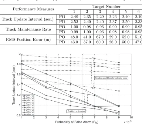
measures for the PO and PD cases are provided in Table 2. The performance improvement for ~ should be observed as it gets longer for any given scenario. In Table 2, when the six benchmark targets are investigated in terms of PO, the track update interval, ~, gets smaller for highly maneuvering targets. For example, for Target 1, ~ = 2.48 and for Target 6, it is equal to 2.19. When Doppler measurements are included into the tracker as in PD case, ~ increases to 2.52 for Target 1 and 2.33 for Target 6. Even when there is no clutter and no missed detection, direct measurements of Doppler provides significant improvement for Track Update Interval. For the case of no clutter

and no missed detection, it is expected that the second performance measure of Track Maintenance Rate to stay constant around 1.0. In the reference case provided in Table 2, this performance parameter stays practically constant for all targets and for both PO and PD cases. The RMS Position Error for PO case across all targets decreases when Doppler velocity is included into the tracker directly, even for cases

when the ~ gets longer. For example, hpos reduces to 43 from 48 for

Target 1, an improvement of 10.4%. The hposfor the most maneuvering

target, Target 6, is reduced to 47 from 51. The probability of detection and the average processing time parameters, as expected, stay nearly constant around unity and 1 ms for all targets and for both PO and PD cases, respectively.

The effect of clutter in the tracker can be observed through the

increasing values of Pf a. In order to investigate the performance

improvement of PD case, a new simulation scenario set is run where

Table 2. Performance measures of TAM unit for P_{f a}= 0 and P_d= 1

(ideal case) where PO and PD indicate the performance for position only and position plus Doppler velocity measurements, respectively.

Performance Measures Target Number

1 2 3 4 5 6

Track Update Interval (sec.) PO 2.48 2.35 2.29 2.26 2.40 2.19 PD 2.52 2.40 2.40 2.37 2.50 2.33 Track Maintenance Rate PO 1.00 0.98 0.96 0.99 0.99 0.95 PD 0.99 1.00 0.96 0.98 0.98 0.95 RMS Position Error (m) PO 48.0 41.0 67.0 29.0 52.0 51.0 PD 43.0 37.0 60.0 26.0 50.0 47.0 1 2 3 4 5 6 7 8 9 10 x 10-5 0.8 1 1.2 1.4 1.6 1.8 2

Probability of False Alarm (P )fa

Track Update Interval (sec.)

Target 1, PO Target 1, PD Target 2, PO Target 2, PD Target 3, PO Target 3, PD Target 4, PO Target 4, PD Target 5, PO Target 5, PD Target 6, PO Target 6, PD

Position only case

Position and Doppler velocity case

Figure 2. Track Update Interval estimation of TAM unit for the

P_dis kept constant at 0.8 and probability of false alarm is varied from

P_{f a} = 1 × 10−5 _{to P}

f a = 9 × 10−5. The five performance measures

are recorded for all six benchmark targets for both PO and PD cases. The average values of the Monte-Carlo runs are provided in Figure 2 to Figure 5. In Figure 2, the performance measure is the Track Update Interval. For Target 1, ~ = 1.81 and for Target 6, it equals 1.43, both

for PO case and Pf a= 1×10−5. When Doppler velocity is incorporated

into the tracker as in PD case, ~ increases to 1.98 for Target 1 and 1.70 for Target 6. Another observation about ~ is that when increasing false

alarm rate from Pf a = 1 × 10−5 to Pf a= 9 × 10−5, ~ values in general

decrease for both PO and PD cases. However, for PD case, the rate

of decrease in ~ for each Pf a is very small with respect to that of PO

case. For example, ~ decreases from 1.81 to 0.98 for Target 1 and PO case. For the PD case and the same target, ~ decreases from 1.98 to

1.83. Depending on the values of Pf a, the rate of increase in track

update interval with respect to PO case varies between 9% (for Target

1, P_{f a}= 1 × 10−5_{) and up to 112% (for Target 3 and P}

f a = 9 × 10−5)

as shown in Figure 2 when Doppler velocity measurement is used. In Figure 3, the performance measure is the Track Maintenance

Rate. For PO case and P_{f a} fixed at 1 × 10−5_{, y}

tmr is 0.84 for Target

1, and ytmr = 0.64 for Target 6. For PD case, relatively increased

values are recorded as 0.88 and 0.86, respectively. For each target,

when Pf a increases, ytmr values decrease for both PO and PD cases.

For instance, for Target 1, ytmr reduces from 0.84 to 0.02 for PO

case. For the same target and PD case, ytmr values decrease from

0.88 to 0.29 with increasing Pf a. However, for PO case, the rate

of decrease in ytmr for each Pf a is more than the reduction in PD

cases. In PD cases, clutter based detections may also be associated with the target of interest due to the fact that the Doppler profiles of the benchmark targets 1, 4, 5 and 6 include zero Doppler values between positive and negative Doppler transitions (zero crossings) [11].

This will lead to a decrease of y_tmr, even if the Doppler velocity

measurements are used. Also, for the benchmark Target 2 and Target

3 which have no zero crossing Doppler velocities, increasing P_{f a} still

results in decreasing values of ytmr although the Doppler velocity

measurements are employed. This is explicitly due to the fact that 3D false position measurements within 4D measurements are very close to the predicted position vector. Such an event occasionally causes those false measurements being in the association region set by the

PDAF algorithm. Therefore, increasing Pf a also decreases the ytmr

for PD case for these targets. Nevertheless, for the PD cases, and for

high values of Pf a, a very significant enhancement in ytmr is achieved

In Figure 4, the performance of h_pos for both PO and PD cases

is provided for increasing P_{f a} values. For example, for Target 1 and

Pf a = 1 × 10−5, hpos is 84 and 58 for PO and PD cases, respectively.

It is recorded as 173 and 79 for Pf a = 9 × 10−5, for PO and PD

cases, respectively. Although ~ increases and, in effect, less number

of revisits provided for the PD case, hpos decreases due to the effect

of the use of Doppler velocity measurements in the TAM algorithm.

Furthermore, when increasing P_{f a}and the maneuver capabilities of the

targets, h_pos values are raised for both PO and PD cases. Still, the

1 2 3 4 5 6 7 8 9 10 0 0.1 0.2 0.3 0.4 0.5 0.6 0.7 0.8 0.9 1

Track Maintenance Rate

Target 1, PO Target 1, PD Target 2, PO Target 2, PD Target 3, PO Target 3, PD Target 4, PO Target 4, PD Target 5, PO Target 5, PD Target 6, PO Target 6, PD

Position only case

Position and Doppler velocity case

x 10-5

Probability of False Alarm (P )fa

Figure 3. Track Maintenance Rate estimation of TAM unit for the

benchmark targets and various Pf a values (Pd= 0.80).

1 2 3 4 5 6 7 8 9 10 40 60 80 100 120 140 160 180 200 220

RMS Position Estimation Error (m.)

Target 1, PO Target 1, PD Target 2, PO Target 2, PD Target 3, PO Target 3, PD Target 4, PO Target 4, PD Target 5, PO Target 5, PD Target 6, PO Target 6, PD

Position only case

Position and Doppler velocity case

x 10-5

Probability of False Alarm (P )fa

Figure 4. RMS Position Error estimation of TAM unit for the

1 2 3 4 5 6 7 8 9 10 1 1.05 1.1 1.15 1.2 1.25 1.3 1.35 1.4

Processing Time (msec.)

Position only case Position and Doppler velocity case

x 10-5

Probability of False Alarm (P )fa

Figure 5. Average Processing Time estimation of TAM unit for

various P_{f a} values (P_d= 0.80).

rate of increment for PD case for each P_{f a} is very small compared to

PO case. The rate of decrease in hpos for PD case is between 20% (for

Target 3, P_{f a}= 1×10−5_{) and up to 67% (for Target 2, P}

f a = 9×10−5)

as shown in Figure 4.

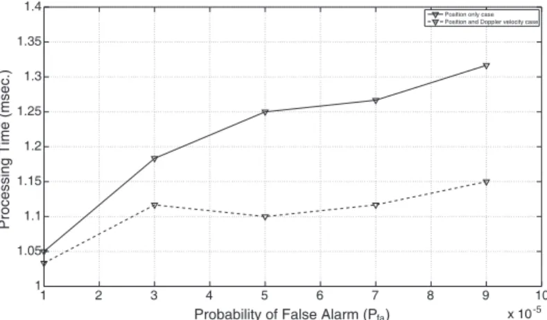
In Figure 5, the average processing time estimation for both PO and PD cases are provided. Under normal operating conditions, it may be expected that the processing time increases in PD cases due to the increasing size of of matrices in TAM algorithms. However, due to the detractive effect of Doppler velocity measurements on false alarms, the

average processing time still decreases up to 12.5% (for Pf a= 9×10−5)

in case of Doppler velocity measurements with respect to PO case. It

is also expected that increasing Pf a should increase tdp, as well. This

expectation is observed in Figure 5. For example, for PO case average

t_dp is 1.05 ms and 1.32 ms for P_{f a} = 1 × 10−5 _{and P}

f a = 9 × 10−5,

respectively. Again, it is obtained for the same false alarms as 1.03 ms and 1.15 ms for PD case.

Probability of detection parameters for both PO and PD cases are quite similar and it approaches the probability of detection value

of the DSP unit (Pd= 0.80).

4. CONCLUSIONS

In this paper, the performance improvement for a multi function phased array radar is investigated when Doppler velocity measurement is incorporated into the track association and maintenance algorithms. Incorporating the Doppler velocity measurements into commonly preferred IMMPDAF estimator with adaptive sampling policy is

simulated and the performance measures are compared with those cases where only 3D position measurements are used. It has been observed that using Doppler velocity measurements in track association and maintenance leads to increased track update interval with the values of between 9% and up to 112%. The RMS position estimation error is decreased by an amount of 20% to 67% with respect to the position only case. The average processing time for position and Doppler velocity case is also decreased by an amount of up to 12.5%.

The results show that Doppler velocity measurements strongly enhance the performance of TAM unit of an MFPAR resulting in saving of energy resources of MFPAR with less number of revisits. Besides, for the same amount of energy, more number of targets can be tracked leading to the increased track capacity. Again, more time and resource can be allocated for the search function. Furthermore, due to the more accurate tracking capability with the Doppler velocity measurements, more successful weapon engagement for the targets under track can be provided.

REFERENCES

1. Bar-Shalom, Y., Multitarget-Multisensor Tracking: Principles and Techniques, YBS, 1995.

2. Blackman, D. and R. Popoli, Design and Analysis of Modern Tracking Systems, Artech House, 1999.

3. Shi, Z.-G., S.-H. Hong, and K. S. Chen, “Tracking airborne targets hidden in blind doppler using current statistical model particle filter,” Progress In Electromagnetics Research, Vol. 82, 227–240, 2008.

4. Bi, S. Z. and X. Y. Ren, “Maneuvering target doppler-bearing tracking with signal time delay using Interacting multiple model algorithms,” Progress In Electromagnetics Research, Vol. 87, 15– 41, 2008.

5. T¨urkmen, I. and K. G¨uney, “Tabu search tracker with adaptive

Neuro-fuzzy inference system for multiple target tracking,” Progress In Electromagnetics Research, Vol. 65, 169–185, 2006. 6. Haridim, M., H. Matzner, Y. Ben-Ezra, and J. Gavan,

“Cooperative targets detection and tracking range maximization using multimode ladar/radar and transponders,” Progress In Electromagnetics Research, Vol. 44, 217–229, 2004.

7. Chen, J.-F., Z.-G. Shi, S.-H. Hong, and K. S. Chen, “Grey prediction based particle filter for maneuvering target tracking,” Progress In Electromagnetics Research, Vol. 93, 237–254, 2009.

8. Sabatini, S. and M. Tarantino, Multifunction Array Radar: System Design and Analysis, Artech House, 1994.

9. Kural, F., F. Arıkan, O. Arıkan, and M. Efe, “Performance evaluation of the sequential track initiation schemes with 3D position and Doppler velocity measurements,” Progress In Electromagnetics Research B, Vol. 18, 121–148, 2009.

10. Kural, F., F. Arıkan, O. Arıkan, and M. Efe, “Incorporating Doppler velocity measurement for track initiation and mainte-nance,” IEE Seminar on Target Tracking: Algorithms and Ap-plications, 107–114, 2006.

11. Kural, F., “Performance improvement of the multiple target tracking algorithms with the incorporation of Doppler velocity measurement,” Ph.D. Thesis, Hacettepe University, 2006.

12. Kural, F., and Y. ¨Ozkazan¸c, “A method for detecting rgpo/vgpo

jamming,” IEEE Signal Processing and Communications Applica-tions Conference, 237–240, 2004.

13. Bizup, D. F. and D. Brown, “Maneuver detection using the radar range rate measurement,” IEEE Transactions on Aerospace and Electronic Systems, Vol. 40, No. 1, 330–336, 2004.

14. Cassassolles, E., M. Ludovic, S. Herve, and B. Tomasini, “Integration of radar measurement attributes in the multiple hypothesis tracker results for track initiation,” Proceedings of SPIE, Signal and Data Processing of Small Targets, Vol. 2759, 397–403, 1996.

15. Lacle, L. and J. Driessen, “Velocity-based track discrimination algorithms,” IEE Target Tracking: Algorithms and Applications, Vol. 2759, 4.1–4.4, 1996.

16. Fitzgerald, R., “Simple tracking filters: Position and velocity measurements,” IEEE Transactions on Aerospace and Electronic Systems, Vol. 18, 531–537, 1982.

17. Farina, A. and S. Pardini, “Track-while scan algorithm in a clutter environment,” IEEE Transactions on Aerospace and Electronic Systems, Vol. 14, 769–778, 1978.

18. Wang, X., D. Musicki, and R. Ellem, “Fast track confirmation for multi-target tracking with doppler measurements,” 3rd International Conference on Intelligent Sensors, Sensor Networks and Information, ISSNIP, 263–268, 2007.

19. Wang, X., D. Musicki, R. Ellem, and F. Fletcher, “Enhanced multi-target tracking with doppler measurements,” Information, Decision and Control, IDC, 53–58, 2007.

and enhanced multi-target tracking with doppler measurements,” IEEE Transactions on Aerospace and Electronic Systems, Vol. 45, 1400–1417, 2009.

21. Kameda, H., S. Tsujimichi, and Y. Kosuge, “Target tracking under dense environments using range rate measurements,” Proceedings of the 37th SICE Annual Converence, International Session Papers, 927–932, 1998.

22. Kosuge, Y., H. Iwama, and Y. Miyazaiki, “A tracking filter for phased array radar with range rate measurement,” Proceedings of 1991 International Conference on Industrial Electronics, Control and Instrumentation (IECON 1), Vol. 3, 2555–2560, 1991. 23. Yeom, S-W., T. Kirubarajan, and Y. Bar-Shalom, “Track segment

association, fine-step IMM and initialization with Doppler for improved track performance,” IEEE Transactions on Aerospace and Electronic Systems, Vol. 40, No. 1, 293–309, 2004.

24. Kirubarajan, T., Y. B. Shalom, W. D. Blair, and G. A. Watson, “IMMPDA solution to benchmark for radar resource allocation and tracking in the presence of ECM,” ECC’97, 1–6, 1997. 25. Bar-Shalom, Y., Estimation and Tracking: Principles,

Tech-niques, and Software, Artech House, 1993.

26. Bar-Shalom, Y., Multitarget-Multisensor Tracking: Applications and Advances Volume II, Artech House, 1993.

27. Campo, L., P. Mookerjee, and Y. Bar-Shalom, “State estimation for systems with sojourn-time-dependent Markov model switch-ing,” IEEE Transactions on Automatic Control, Vol. 36, No. 2, 238–243, 1991.

28. Yang, C. and C. F. Lin, “Discrete-time mode filters for markovian jump processes”, The First IEEE Regional Conference on Aerospace Control Systems Proceedings, 613–617, 1993. 29. Watson, G. A. and W. D. Blair, “Tracking performance of a

phased array radar with revisit time controlled using the IMM algorithm,” IEEE National Radar Conference, 160–165, 1994. 30. Blair, W. D., G. A. Watson, S. Hoffman, and G. L. Gentry,

“Benchmark problem for beam pointing control of phased array radar against maneuvering targets in the presence of ECM and false alarms,” Proceedings of American Control Conference, 2601– 2605, Seattle WA, 1995.

31. Daeipour, E., Y. Bar-Shalom, and X. Li, “Adaptive beam pointing control of a phased array radar using an IMM Estimator,” Proc. American Control Conference, 2093–2097, Baltimore, MD, 1994.