Implementation of Johansen procedure in the estimation of demand for M1 and M2 using the Turkish data

. m jm m m M ^ m m m m Of semamo FQi M l m B wa

USING T H E TURK ISH D A T A

SMuir.ittsd is ffes Dspartjsent of Scsnsmics

;nij tfe®

af Esanojsiss fesd

Surni

Sssasss^

!]-) pgjftia) 3! ??i'S Ba-:jB3iijriSSj3

lOr the Degi'efe 0

M A S T ER D r A R T S

_M

E tO ^ G M IC S

H G

. O ' S s

f s s s

IM P L E M E N T A T IO N OF J O H A N S E N P R O C E D U R E

IN T H E E S T IM A T IO N OF D E M A N D FO R M l A N D M 2

U SIN G T H E T U R K IS H D ATA

A Thesis

Submitted to the Department of Economics

and the Institute of Economics and Social Sciences

of Bilkent University

In Partial Fulfillment of the Requirements

for the Degree of

MASTER OF ARTS IN ECONOMICS

By

Emre OZDENOREN

October, 1993

VT

K{

:s

o<

î

I certify that I have read this thesis and in rriy opinion it is fully ade­ quate, in scope and in quality, as a thesis for the degree of Master of Arts in Economics.

P rof. DrOSub^ey Togan

I certify that I have read this thesis and in rny opinion it is fully ade­ quate, in scope and in quality, as a thesis for the degree of Master of Arts in Economics.

I certify that I have read this thesis and in my opinion it is fully ade­ quate, in scope and in quality, as a thesis for the degree of Master of Arts in Economics.

Dr. Kivilcirn. Metin

Approved by the Institute of Social and Economic Sciences

Acknowledgements

I would like to thank Prof. Dr. Siibidey Togan for leading me to this

study and for his encouragements and recommendations during the preparation

of the study. I also wish to thank to Assist. Prof. Dr. Osman Zaim and Dr.

Kıvılcım Metin for their invaluable help.

Finally, 1 wish to thank to my mother who provided me a comfortable

ABSTRACT

IMPLEMENTATION OF JOHANSEN PROCEDURE IN

THE ESTIMATION OF DEMAND FOR M l AND M2

USING THE TURKISH DATA

M A in Economics

Supervisor: Prof. Dr. Subidey T O G A N

October 1993, 60 pages

This study aims at estimating the money demand function for Turkey using

quarterly data. Estimation is done, for both M l and M2, using Johansen

procedure, which is a variate of the theory of cointegration.

The results of the Johansen procedure shows that real income is positively

and expected loss is negatively related with demand for Ml and M2. Also, some

linear restrictions are tested, by restricting the money demand coefficients.

The results of these tests show that Tobin-Baumal model and unit elasticity

of income are rejected for both M l and M2.

Key Words : money demand, cointegration, level of integration, stationarity.

Johansen procedure.

ÖZET

PARA TALEP FONKSİYONUNUN TÜRKİYE İÇİN

JOHANSEN M ETODUYLA TAHMİN EDİLMESİ

Emre Ö ZD E N Ö R E N

Yüksek Lisans Tezi

Ekonomi ve Sosyal Bilimler Enstitüsü

Tez Yöneticisi: Prof. Dr. Sübidey T O G A N

Ekim 1993, 60 Sayfa

Bu çalışmada üç aylık veriler kullanılarak Türkiye için para talep fonksiyonu

tahmin edilmiştir. Tahminlerin yapılmasında Johansen metodu kullanılmıştır

ve tüm hesaplamalar Mİ ve M2 için tekrarlanmıştır.

Johansen metodu kullanılarak yapılan tahminlerin sonucunda, hem Mİ

hem M2 için, reel gelirlerin katsayısı pozitif ve paranın beklenen kaybının

katsayısı negatif olarak bulunmuştur. Ayrıca, bazı doğrusal kısıtlamalar test

edilmiştir. Bu testlerin sonuçlarına göre Tobin-Baumal modeli ve birim gelir

esnekliği hipotezleri, hem Mİ hem de M2 için reddedilmiştir.

TABLE OF CONTENTS

2.2.1 Stationarity, Unit Roots and Orders of Integration 2.2.2 Testing for the Level of Integration

2.2.3 A Maximum Likelihood Approach 2.2.4 Testing Linear Restrictions

2.2.5 Weak Exogeneity

3 Empirical Study on Money Demand Functions for M l and M2 3.1 Testing for Unit Roots

3.2 Testing for the Number of Cointegrating Vectors

3.3 Results of the Johansen Procedure

111 VI 1 2 2 10 10 11 13 18 19 21 21 23 24 IV

3.4 Testing Linear Restrictions on ¡3 25

3.5 Testing Linear Restrictions on a 28

Conclusion 32 References 36 Data Sources 39 Appendix A 40 Appendix B 42 Appendix C 44 Appendix D 46

LIST OF TABLES

Table 1: Unit Roots Tests for Money, Income and Expected Loss 22 Table 2: Likelihood Ratio Statistic for Ml and M2 for the Number of

Cointegrating Vectors 23

Table 3: H matrix for the unit income elasticity restriction 26 Table 4: H matrix restricting coefficient of REALY as 1/2 and

of EL a s -1/2 27

Table 5: A and B matrices for testing a2 = 0 29

Table 6: A and B matrices for testing «3 = 0 29

Table 7; A and B matrices for testing «2 = «3 = 0 30 Table 8: Results of multicointegration analysis for M l 40

Table 9: Results of multicointegration analysis for M2 41

Table 10; Results of multicointegration analysis for M l under the unit income

elasticity restriction 42

Table 11: Results of multicointegration analysis for M2 under the unit income

elasticity restriction 43

Table 12: Results of multicointegration analysis for M l under the hyphoteses that coefficient of real income is 1/2 and coefficient of expected loss is -1/2 44 Table 13: Results of multicointegration analysis for M2 under the hyphoteses that

coefficient of real income is 1/2 and coefficient of expected loss is -1/2 45

that «2 = 0 46 Table 15: Results of multicointegration analysis for M l under the hyphoteses

that «3 = 0 47

Table 16: Results of multicointegration analysis for M l under the hyphoteses

that «2 = «3 = 0 48

Table 17: Results of multicointegration analysis for M2 under the hyphoteses

that «2 = 0 49

Table 18: Results of multicointegration analysis for M2 under the hyphoteses

that 03 = 0 50

Table 19: Results of multicointegration analysis for M2 under the hyphoteses

that «2 = <3:3 = 0 51

Table 14: Results of rnulticoiritegration analysis for M l under the hyphoteses

1

Introduction

The determination of a relationship between money, income, interest rates

and other related variables and the stability of such relationships have been

an important topic in the literature.

In this thesis, the long run demand for money function in Turkey

for the period 1977(1)-1989(4) has been investigated using a maximum

likelihood method suggested by Johansen(1988), which is a variate of the

theory of cointegration. This method also gives the opportunity to test some

economically meaningful hypoteses.

Cointegration analysis states that economic series which are non-

stationary may drift together as a group. If there is such a relationship between

a set of variables, this analysis helps to discover it. If an economic theory is

correctly specified then these variables will be related with each other with

constant parameters, so these variables would not drift increasingly further as

time goes on. But if the variables are not cointegrated then there should be

doubts about the underlying economic theory, or at least the model.

This study is organized in the following way. Section 2 gives the necessary

briefly, In 2.2 econometric framework is discussed. Here the theory of unit roots

and cointegration is overviewed, and tlie methodology suggested by Johansen

is described.

In section 3 empirical results are reported. In this section also the

results of various hypoteses tests are given, which compares the Turkish money

demand function with the theory of money demand. Lastly, all these results

2

Theoretical Background

2.1 Economic Framework

One of tfie earliest approaches to the demand for money is the quantity theory

of money. Quantity theory starts with the equation of exchange which can be

written as,

M V = PT ₍₁₎

where M is the quantity of money, V is the velocity of circulation, P is the

price level, and T is the volume of transactions. In this equation M, P, and

T are directly measurable, but V is implicitly defined by (1). If we assume

that velocity, V, is determined by technological or institutional factors and

therefore is relatively constant then we can view (1) as a demand function for

money. Then from (1) we see that demand for real balances is proportinal to

the volume of transactions.

Since Angelí (1936), monetary economists express the quantity equation

in terms of income transactions rather than gross transactions. Let y be the

national income at constant prices. We can write the quantity equation in

income form as.

where M is the quantity of money as before, but V is now defined as the average

number of times per unit time that the money stock is used in making income

transactions.

Keynes (1936) modified this simple money demand function by introduc­

ing the speculative motive for holding money, together with the trancactions

motive. In the speculative motive approach, money and bonds are seen as

alternative assets. As bond holding depends on the rate of return on bonds,

interest rate enters into the demand equation for money. Once the interest

rate is introduced, one does not need to assume constant velocity anymore.

Transactions approach emphasizes the role of money as something that

everybody will accept in exchange as ‘general purchasing power’. But there

must also be something which can serve as a temporary abode of purchasing

power during the time that passes between sale and purchase. This aspect of

money can be seen from the cash-balance equation.

M = kPy ₍₃₎

where k is the ratio of money stock to income. Apperantly k is the reciprocal of

V, a simple mathematical transformation, but it stresses the role of money as

suggests treating money as part of capital or wealth theory.

Friedman (1956) restated the quantity theory of money. He treated

money like any other asset yielding a flow of services. He distinguishes between

ultimate wealth holders to whom money is an asset which they choose to

hold their wealth, and enterprises to whom money is a producer’s good like

machinery or inventories.

For ultimate wealth holders demand for money may be expected to be a

function of;

(i) Total wealth,

(ii) The division of wealth between human and non-human forms,

(iii) The expected rates of return on money and other assets,

(iv) Other variables determining the utility attached to services rendered by

money relative to those rendered by other assets.

Baumal (1952) and Tobin (1956) applied inventory-theoretic considera­

tions to the transactions demand for money. Their studies led to the well-

known square-root law, where average money holdings are given by.

M = (26r/r)i/2 (4)

both sides of equation (4) by price level makes the demand for money depend

on interest rate, real brokerage charges and the level of real transactions. Miller

and Orr (1966) extended this analysis to allow for uncertainty in cash flows.

Their analysis showed that a firm’s average money holdings depends on the

variance of its cash flow.

Some other studies have tried to reformulate Keynes’ speculative motive

in terms of portfolio theoryh But there is a serious problem with this approach.

If there is a riskless asset, such as a savings deposit, which is paying a higher

rate of return on money, than money is a dominated asset and will not be held.

So one must combine the portfolio approach with transaction costs in order to

find an asset demand for money.

In order to estimate a money demand function empirically, one needs

explicit variables which measure money and its determinants. The first step

is to decide what can be accepted as money. In general, theories based on

the transactions motive lead to a narrow definition of money, which includes

currency and demand deposits.

If one moves away from the transactions view, and assumes that money IfTobin (1958)

yields some unspecified services, then the definition of money is even less clear

because there may be other assets which yield the same services. In this study

two definitions of money are considered. The first one is M l, consisting of

currency plus demand deposits, and the second one is M2, consisting of M l

plus time deposits. M l can be seen as a variable which reflects the transactions

view of the world and M2 can be seen as a variable which also reflects the asset

use of money.

The level of transactions is typically measured by the level of income or

gross national product, which is also the case in this study.

Another measurement issue is the oportunity cost of holding money.

Here, the own rate of return on money and the rate of return on assets

alternative to money must be considered. For the latter under transactions

view, in general, some interest rate on a savings deposit or a combination

of such interest rates is used. But it must be noted that consumption of

goods is an alternative to holding money and inflation is the rate of return on

consumption goods. In this study consumption is taken as the only alternative

to money. This is an assumption mostly utilized for the financially repressed

where

-■M. =

_{- T)}

,.^^^nu2S m LL nTD (l-T )

DD: Demand Deposits

TD; Time Deposits

T; Tax Rate on Interest Income

The own rate of return on money is defined as follows for M l and M2:

roD- Interest on Demand Deposits

ttd· Interest on Time Deposits

The equation estimated in this study is given as,

In M = a In i/ + bEL ₍₅₎

where EL, or expected loss is defined as expected inflation minus interest on

money. This is in fact negative of the real rate of return on money. The

equation above can be obtained from the square-law by taking the logarithm,

and replacing the amount of transactions with income, and real interest rate

by expected loss. Expected signs are positive for income and negative for EL.

inflation in any period is the inflation rate which occurred in the previous

2.2

Econometric Framework

2.2.1 Stationarity, Unit Roots and Orders of Integration

A time series [xt is stationary if its mean, E{xt), is independent of t, and

its variance, E[xt — E(xt)Y is bounded by some finite number and does not

vary systematically with time. A stationary series tends to return to its mean

and fluctuate around it within a more or less constant range whereas a non-

stationary series would have a different mean at different points in time.^

If a series must be differenced d times before it becomes stationary, then

it is said to be integrated of order d, denoted by 7(d).Alternatively, we can

say that a series is 1(d) if it has a stable, invertable, non-deterministic ARMA

representation after differencing d times.

We can write an 1(d) series as

(1 - L)U (L)xt = 0(L)et ₍6)

where L is the lag operator, <I>(L) and 0(L) are polynomials in the tag operator

and et is a stationary process. The roots of the polynomial, (1 — L)'^<f)(z) = 0,

are called unit roots. As there are d roots oi z = \ testing for the order of ^For more information on the topics of this section see Engle and Granger (1987).

integration of a series is also called testing for the unit roots.

In general, if we take two series integrated of different orders, any linear

combination will be integrated at the highest of the two orders of integration.

An exception to this rule is where the low-frequency components of two series

exactly offset each other and give a stationary linear combination. This is the

case of a set of cointegrating variables. If a set of series are cointegrated, in

the long run, they move closely together, even though they are individually

trended.

The components of a vector Xt are said to be cointegrated of order d, b,

denoted by Xt ~ CI{d, b), if:

(i) all components of Xt are I{d) and,

(ii) there exists a vector a(y^ 0) such that Zt = (x'Xt ~ I[d — b),b > 0.

2.2.2 Testing for the Level of Integration

Consider the following autoregressive representation of a variable Xt'.

— >^0 + + ^2^t-2 + ··· + (₇)

where Ut is a white noise stationary term.

Now, reparametrise (7):

n+l n+l n+l

A^i — Ao + A,· — l)xt_i — Ai)Aa:i_^] + Ut

i= l z = i i= z

(8)

Consider the regression

Axt = /7o + /3ixt-i + ^ aiAxt-i + Ut (9)

1=1

Now, comparing (7), (8) and (9), we can conclude that stationarity requires

[3i < 0, while if Xt is non-stationary, than would be equal to zero. The

latter will also mean that the sum of the autoregressive parameters A,· in (7)

would be unity, implying that the series would have a unit root.

Then, one way of testing for stationarity would be to estimate a regression

of the form (9), and test the hyphoteses that /?i = 0. This can be done using

the ratio of /3, to its estimated standart error. This ratio is the augmented

Dickey-Fuller Statistic(ADF).

The distribution of ADF is not Student’s t so Fuller(1976) has tabulated

critical values for this statistic by Monte Carlo methods. The number of lags

of Axt is normally chosen to ensure that the regression residual is white noise.

In this study four lags are used because data used is quarterly.

If no lags of Axt are used, then the ratio is called Dickey-Fuller (DF)

statistic. The critical values for DF and ADF statistics are the same for one

variable case.

In order to test for second order integration, we have to run the following

regression:

n—1

= 7o + 7i Aa;t_i + ^ '^iA'^xt-i + Ut (10)

¿=1

In this case, similarly, we test the null hypoteses that Axt is stationary, 71 = 0,

against the hypoteses that 71 < 0.

2.2.3 A Maximum Likelihood Approach

One problem here is to know the number of cointegrating combinations which

may exist between a set of variables. If one consider two variables each

integrated of order one, Xt ~ / (1) and Yt ~ -f(l); we can show that there

is a unique parameter a such that

u t ^ X t - aYt ~ / (0) ₍

₁₁

To see this assume there is another cointegrating parameter ¡3:

wt = X t - ßYt ~ / (0) (12₎

Adding and subtracting fiYt in (11) we can obtain:

ut - wt - {a - /3)Yt (13)

According to our assumption Ui and Wt are both 7(0) while Yt is 7(1).

This can hold only if a — 13. So, a is unique. But when we consider more than

two variables, it is not possible to guarantee the uniqueness of the cointegrating

vector.

The original approach was to assume a unique cointegrating vector. This

approch was developed in the inlluencial work of Engle and Granger (1987).

Johansen(1988) suggests a method for estimating all the cointegrating vectors

and for constructing some statistical tests. He proposes the following data

generation process of a vector of N variables X\

Xt — H iX i-i + ... + WkXt-k + Ci (14)

where each Hi is an (N x N) matrix of parameters. This equation can be

reparametrised in the error correction form as:

X X t = E iA X t-i + ... + r^t-iAXi-fc+i + TkXt-k + (15)

where

Ej- — —7 + Hi + ...Hi; i — l...k.

So l\ is a long run solution to (14).

Now, if Xt is a vector of / (1) variables, then the left hand side of (15) is

/(0 ). At the right hand side all terms, other than the final term, are also / (0).

This implies that the last term must also be /(0 ), FkXt-k ~ -^(0)· This means

that either X contains a number of cointegrating vectors or is a matrix of

zeros. Now, we define two N xr matrices a and ^ such that

It is easy to see from here that the columns of

(3

parameter vectors for Xt, \i X consists of variables integrated of order one

then r must be at most A^ — 1, s o r < A ^ — 1.

In his paper Johansen gives the following theorem.

Theorem: The maximum likelihood estimate of the space spanned by ¡3 is

the space spanned by the r canonical variates corresponding to the r largest

squared canonical correlations between the residuals of Xt-k and XXt corrected

for the effect of the lagged differences of the X process. The likelihood ratio

test statistic for the hyphoteses that there are at most r cointegrating vectors

IS

N

-2 \ n Q ^ - T I n ( l - A i )

i=r-\-l

where A^+i-.-Aat are the {N — r) smallest squared canonical correlations. (16)

After this Johansen shows that the likelihood ratio test has an asymptotic

distribution which is a function of an — r dimensional Brownian motion and

he tabulates a set of critical values which will be correct for all the models.

He also demonstrates that the space spanned by ^ is consistently estimated

by the space spanned by ß.

According to the Johansen’s procedure we first regress A A i on the lagged

differences of A A j which gives a set of residuals Rot- We then regress Xt-k on

the lagged differences of A X t-j which gives another set of residuals Rkt- The

likelihood function is then proportional to T

L {a ,ß ,ü ) = \i\\-'^l^exp[-ll2Y{Rot + aß'Rkt)'n-\Rot + aß'Rkt)] (17) t=i

where T is the number of observations and is the covariance matrix of

Assuming /3 as fixed we can maximize over a and H by regressing Rot on

—/3'Rkt ■ This will give us

&{ß) = -Sokßiß'Skkß)-1

n{ß) = Soo - Sokßiß'Skkß)-^ß'Sko 16

where

Si, = T - ' R.,R'„. i , f = 0, k

After substituting these into the likelihood function, resulting function

will be proportional to . So maximizing the likelihood function may

be reduced to minimising

|5’oo - Sokß{ß'Skkß)-^ß'Sko\ (18)

with respect to ß.

This can be done by solving an eigenvalue problem. The matrix $ is

obtained as a set of eigenvectors with a corresponding vector of eigenvalues A.

The columns of ^ are significant if the corresponding eigenvalue is significantly

different from zero. Let the elements of Aj· be ordered as;

Ai > A2 > ··· > Aat-1 and let the columns of ^ be ordered accordingly.

Then the eigenvalues are defined such that the maximum likelihood estimate

of i) is given by:

N

= i5ooi I I P --'■■)■ (19)

i=\

Now, if we want to test the following null hyphoteses:

Hq : Ai = 0,2 = r + 1, ...,N - 1,

we have to restrict the estimate of ft as:

W = l '5 'o o in ( l- - ^ 0 · (20)

Then we can form a likelihood ratio statistic for the null hyphoteses of at most

r cointegrating vectors as

N

where

LR(N - r) = ~2hi{Q ) = - T ln(l - A,·)

2=r-f-l

Q _ restricted maximised likelihood unrestricted maximised likelihood

Johansen (1989) gives the critical values for this statistic.

(21)

2.2.4 Testing Linear Restrictions

Johansen(1988) also demonstrates how linear restrictions can be tested on the

parameters of the cointegrating vector. He considers linear restrictions on ¡3

which reduce the number of independent cointegrating parameters from N to

S where S < N. In general the restrictions will be written in the following

form:

Ho:

₂₂

where H is an (NxS) matrix of full rank equal to S and (j) is an (Sxr) matrix of

unknown parameters. Since H is known, we will replace ¡3 with H<f> to obtain

The restricted estimation will produce a set of eigenvalues, > A2 >

... > A*. This will give us a test based on the first r cointegrating vectors: an estimate (¡)*. The restricted estimate of ¡3 will then be given by ¡3* = H(f>*.

LB-\

(N -

5·)] = -21,i((3) = r ; ^ l n ( l - A>)/(1 - A,.)

which has an asymptotic chi-square distribution with r(N-S) degrees of

freedom.

2.2.5 Weak Exogeneity

Exogeneity is a basic feature of ernprical modelling and it is studied in Richard

(1980), Hendry and Richard (1982, 1983) and Engle, Hendry and Richard

(1983). Suppose, Xt is a vector of observations on all variables in period t,

and X t-i — ■ Then the joint probability of the sample Xt may be

written as

(24)

where 0 is a vector of unknown parameters.

In order to simplfy this very general formulation we have to marginalize

the data generating process (DGP). This DGP contains more variables than

we can deal with in practice, so we choose a subset of variables. Secondly, given

this choice of variables of interest, we must select a subset of these variables to

be the endogenous variables (Yt). These are then determined by the remaining

variables (Zt) of interest.

We can represent these two assumptions by the following factorisation:

D{xt\Xt-ue) = A{Wt\Xt

a)B{Yt\Yt.u Zt

^)C{Zt\Yt-u Zt-,

₇

A specifies the determination of W, the variables of no interest, as a function

of all the variables Xt- B gives the endogenous variables of interest Yt as a

function of lagged Y and the exogenous variables Zt. C gives the determination

of the exogenous variables Zt as a function of the lagged endogenous and

exogenous variables.

The conditioning assumptions require that the Zt variables are at least

weakly exogenous. This means that Zt is independent of Yt, which is assumed

in term C.

3

Empirical Study on Money Demand Func­

tions for M l and M 2

In this study quarterly data for the period 1977(1)-1989(4) is used. The data

consists of M l, M2, real income, price index, interest on demand deposits,

interest on one year time deposits, quantity of demand deposits, quantity of

time deposits, and tax on interest income^.

3.1

Testing for Unit Roots

Estimation procedure begins with the determination of the level of integration

for the relevant variables. This is important because if any of the variables

are stationary than we can not talk about cointegration between that variable

and the other variables.

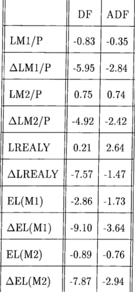
The level of integration is tested using DF and ADF tests for logarithm of

M l (L M l/P ), logarithm of M2 (LM 2/P), logarithm of real income (LREALY),

expected loss for M l (E L (M l)) and expected loss for M2 (EL(M2)).

The null hyphoteses in each case is that the variable in question is 1(1).

Naturally, if first difference of a variable is 1(1), then the variable itself is 1(2).

The 5 % rejection region for both Dickey-Fuller and Augmented Dickey-Fuller ®See the data sources.

Table 1: Unit Root Tests for Money, Income and Expected Loss DF ADF L M l/P -0.83 -0.35 A L M l/P -5.95 -2.84 LM 2/P 0.75 0.74 A L M 2/P -4.92 -2.42 LREALY 0.21 2.64 ALREALY -7.57 -1.47 E L(M l) -2.86 -1.73 A E L (M l) -9.10 -3.64 EL(M2) -0.89 -0.76 A EL(M2) -7.87 -2.94

statistics are the same, D F orA D F < —2.93'*.

Looking at Table 1, we can conclude that Dickey-Fuller test rejects the

null hypoteses for the first differences of the variables, but both of the tests

support the hypoteses that all of the variables in levels are 1(1). This means

that we can use the Johansen procedure described previously. 4 Fuller (1976)

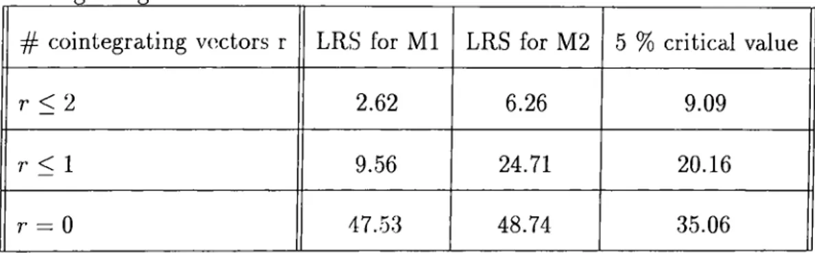
Table 2: Likelihood Ratio Statistic for M l and M2 for the number of Cointegrating Vectors

# cointegrating vectors r LRS for M l LRS for M2 5 % critical value

r < 2 2.62 6.26 9.09

r < 1 9.56 24.71 20.16

r = 0 47.53 48.74 35.06

3.2

Testing for the Number of Cointegrating Vectors

As all the variables of interest are 1(1), it is possible to implement the procedure

described in the previous chapter. In order to implement the procedure, it

seems plausible to use fourth order lags for the vector autoregression, because

the data used is quarterly.

From Table 2 we see that for M l the hyphoteses that r = 0 is rejected

at 95 % significance level, while the hyphoteses of one or more cointegrating

vectors is not. So we can conclude that there is a single statistically significant

cointegrating vector.

For M2 the hyphoteses that r = 0 and r < 1 are rejected at 95 %

significance level, while the hyphoteses of two cointegrating vectors is not. So

here we can conclude that there is definitely one, but possibly there are two

statistically significant cointegrating vectors.

3.3

Results of the Johansen Procedure

Now, in the light of section (2.2.3), we will set up a VAR model which allows

for fourth order lags of each variable, a constant and a trend. This means each

equation will consist of 14 variables. The result are reported in Appendix A

for M l, and M2.

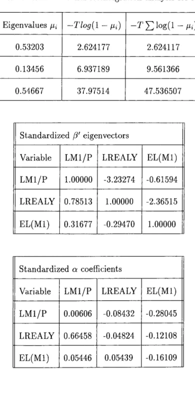
The eigenvectors presented in Appendix A are normalized by real M l

for the first, by real income for the second, and by expected loss for the third.

From the first row of one cointegrating combination represents a real money

demand relationship as, (1, -3.23, 0.61).

So this gives us the following relationship for the long-run solution for

real M l balances.

LMl/ P

S.23LREALY - OSIEL(MI)

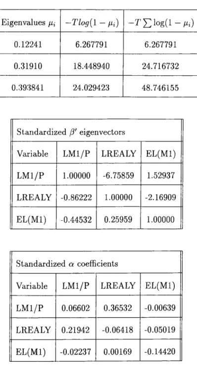
The eigenvectors presented in Appendix A are normalized by real M2

for the first, by real income for the second, and by expected loss for the third.

From the first row of one cointegrating combination represents a real money

demand relationship as, (1, -6.75, 1.52).

So this gives us the following relationship for the long-run solution for

real M2 balances.

LM2/P = Q.75LREALY - 1.52EL{M2) (27)

From the previous section we know that there is a second possible

cointegrating vector for M2. This can be solved by eliminating LM 2/P from

the second row using the first row. The solution of this process will give us the

folowing relationship between the real income and the expexted loss on M2.

LREALY = -0 A 7E L {M 2 ) (28)

3.4

Testing Linear Restrictions on

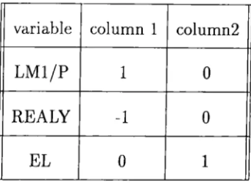
Firstly, we restrict /3 such that the long-run income elasticity of income is

unity. In other words the coefficients of real money and income are equal

with opposite sign. The hypoteses is formulated as ^ = H(j) where II is the

restriction matrix of dimension (p x s) and </> is a (s x r) matrix of unknown

parameters.

Eigenvalues and eigenvectors under this restriction is given in Appendix

Table 3: H matrix for the unit income elasticity restriction

variable column 1 column2

L M l/P 1 0

REALY -1 0

EL 0 1

B for both M l and M2. Using this data we can calculate the test statistic for

M l as;

-2lriQ = = 5 1 [/n (l-0 .1 8 )-/n (l-0 .5 4 )] = 30.09

which will be compared with X^95r(p_s) = X^gs.i = 3.84 where p-s indicates

the number of restrictions on /3 and r is the number of cointegrating vectors.

Therefore the hypoteses of unit income elasticity for M l demand is rejected at

95 % significance level. Also, calculating the same statistic for M2 will yield:

-2 ln Q = T X ) " ^ J / n ( l - / i * ) - / n ( l - / / i ) ] = 5 1 [ /n ( l - 0 .3 1 ) - /n ( l - 0 .3 9 ) ] = 5.86

Comparing this value with 3.84, we also reject this hyphoteses for M2 at 95 %

signihcance level.

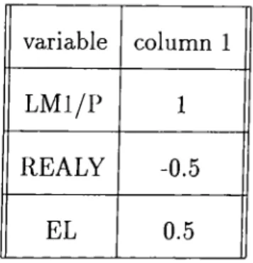
Secondly, we restrict ¡3 such that the cefficient of REALY is 1/2 and the

coefficient of EL is -1/2, which may be looked as a test of the Tobin-Baumal

Table 4: II matrix restricting coefficient of REALY as 1/2 and coefficient of EL as -1/2 variable column 1 L M l/P 1 REALY -0.5 EL 0.5

money demand function.

Eigenvalues and eigenvectors under this restriction is given in Appendix

C for both M l and M2. Calculating the test statistic for M l will give:

-2 ln Q = T J ] ; ^ j [ / n ( l - ^ i ) - / n ( l - p i ) ] = 5 1 [/n (l-0 .1 2 )-/n (l-0 .5 4 )] = 34.17

which will be compared with X^9Sr(p_s) = xi95,2 — 5.99 where p-s indicates

the number of restrictions on ^ and r is the number of cointegrating vectors.

Therefore the hypoteses that coefficient of REALY being equal to 1/2 and

coefficient of E L (M l) being equal to -1/2 is rejected at 95 % significance level.

Calculating the same statistic for M2 will yield;

-2 ln Q = = 5 1 [/n (l-0 .7 8 )-/n (l-0 .3 9 )] = 15.81

The hypoteses is rejected also for M2.

3.5

Testing Linear Restrictions on

Satisfactory modelling requires weak exogeneity of the regressors. Weak

exogeneity can be tested by putting restrictions on a matrix.

One can test weak exogeneity, by restricting a of the form a = A4> where

A is a (p X m) matrix. Also define B which is (p x (p-rn)) and othogonal to

A, B ’A =0. Therefore, B'a = 0 indicating that some of the rows of a should

be zero.

Here, we will consider tests for weak exogeneity of real income («2 =

0) and expected loss («3 = 0). Finally a joint hyphoteses of (o;2 — =

0) is considered. The eigenvalue and eigenvectors under this restrictions are

reported in Appendix D.

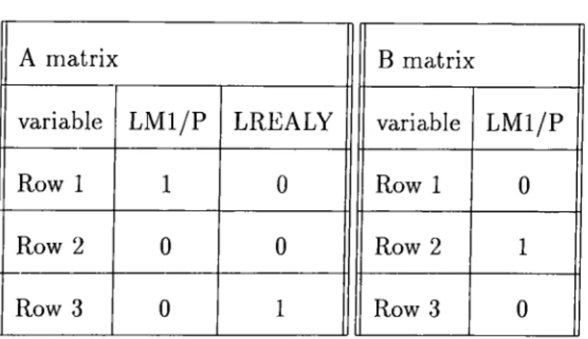
For, the three cases the restriction matrices A and B are shown in tables

5,6 and 7 respectively.

Test statistic for 02 = 0 is;

-2 ln Q = 51[/n(l - 0.21) - /n (l - 0.54) = 27.2]

The test statistic is asymptotically distributed as with f=r(p-m ) degrees of

freedom. Comparing this value with Xo.95,i> income is not

Table 5: A and B matrices for testing CI2 = 0

A matrix B matrix

variable L M l/P LREALY variable L M l/P

Row 1 1 0 Row 1 0

Row 2 0 0 Row 2 1

Row 3 0 1 Row 3 0

Table 6: A and B matrices for testing as = 0

A matrix B matrix

variable L M l/P LREALY variable L M l/P

Row 1 1 0 Row 1 0

Row 2 0 1 Row 2 0

Row 3 0 0 Row 3 1

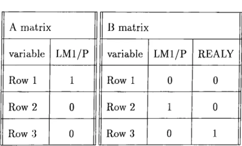
Table 7: A and B matrices for testing a 2 = 0:3 = 0

A matrix B matrix

variable L M l/P variable L M l/P REALY

Row 1 1 Row 1 0 0

Row 2 0 Row 2 1 0

Row 3 0 Row 3 0 1

weakly exogenous for the long run demand for M l.

Test statistic for 0:3 = 0 is:

-2 ln Q = 51[/n(l - 0.54) - ln{l - 0.54)] = 0

Comparing with Xo.95,1 shows that expected loss is weakly exogenous.

Test statistic for «2 = 0:3 = 0 is;

-2 ln Q = 51[/n(l - 0.19) - ln{l - 0.54)J = 28.52

Comparing with Xo.95,2 shows that the joint hyphoteses of weak exogeneity is

also rejected.

For M2 the same statistics can be reported as follows:

Test statistic for a2 — 0 is:

-2 ln Q = 51[/n(l - 0.31) - ln{\ - 0.39) = 6.06]

Xo.95,1 suggests that real income is not weakly exogenous for the long run

demand for M l.

Test statistic for 0:3 = 0 is:

-2 ln Q = 51[/n(l - 0.38) - ln{\ - 0.39)] = 0

Comparing with Xo,95,i shows that expected loss is weakly exogenous.

Test statistic for 0:2 = 0:3 = 0 is:

-2 ln Q = 51[/n(l - 0.31) - /n (l - 0.39)] = 6.06

Comparing with X o .9 5 ,2 shows that the joint hyphoteses of weak exogeneity is

not rejected.

4

Conclusion

In this study, the main aim was to test the money demand function for

the period 1977(1 )-1989(4). This is done by using the Johansen procedure.

This procedure is in essence a maximum likelihood approach to theory of

cointegratiori. This method has some advantages against Engle and Granger

two step procedure. Engle and Granger two step procedure is done by

estimating a static regression and ignoring the dynamics in the first step. The

complete omission of dynamics in the first step creates problems since dynamics

are important in finite samples to reduce bias in both short-run and long-run

coefficient estimates. In addition, a two-step estimating procedure does not

have well defined limiting distributions, but the dynamic models often allow

to use the standart Normal asymptotic theory."

In money demand studies highly aggregated time-series data are used.

Initially the data were annually in most studies but in recent studies the focus

is on shorter periods. Following this path quarterly data is used in this study,

which is the shortest period available in Turkey. The main reason for using

shorter periods is that these are more useful for guiding monetary policy. ®For details see Banerjee and others (1986), Stock (1987), and Stock and West (1988).

I'he results showed that M l, M2, real income and expected loss terms

are all 1(1). For bol.h Ml and M2 tlu' resuls of the analysis suggested

that money is cointegrated with real income and expected loss. 'I'liis is

strong evidence supporting quantity theory of money which is suggesting a

relationship between these variables. Existence of a long-run relationship

for money demand is confirmed by the tests concerning the number of

cointegrating vixtors. d’here is at least one cointegrating v(x:tor for both Ml

and M2 for stire.

We have argued before that quantity theory in the form formulated by

Friedman requires the money demand to be a function of income, expected

interest rate on money and expected interest rates on alternative assets. In

our formulation the alternative interest rate is taken as inflation, 'l lui rationale

behind this is in a financially repressed economy the only alternative to money

is consumption. Under this assumption expected loss is defined as inflation

minus nominal interest rate on money. This is in fact negative of the real

interest rate on money.

We expect the coefficient of income to be positive. In Friedman’s

formulation coefficient of return on money is expected to be positive and

coefficients of alternative rates are expected to be negative. In our formulation

the coefficients of inflation and interest rate on money are restricted to have

the same magnitude with opposite signs. Under this restriction we know that if

real interest rate on money increases then demand for money increases. Thus,

we expect the sign of expected loss to be negative.

The results of the Johannsen procedure supports the arguments stated

above. The signs of the variables are as expected. Sign of real income is

positive and sign of expected loss is negative, although the magnitude of

income term is larger than expected. The results also gave some evidence of a

second cointegrating vector for M2. This vector suggests a long run negative

relationship between income and expected loss.

Tests of linear restrictions on ^ is used to restrict the money demand

coefficients. Tobin-Baumal model is rejected for both M l and M2. This test

is performed by restricting the coefficients of real income and expected loss to

1/2 and -1/2 respectively. Unit elasticity of income is rejected for M l, it is

also rejected for M2. This test is performed by restricting the coefficient of

real income to one.

Tests of weak exogeneity are done by imposing restrictions on a. It is

worth rioting that income seems not to be weakly exogenous, but expected

loss is weakly exogenous for both M l and M2. Also a joint test is performed.

For M l income and expected loss are not weakly exogenous jointly. For M2,

income and expected loss are weakly exogenous jointly. This may be taken as

evidence for the fact that our model for M2 is valid. And, using M2 gives better

and econrnically more interpretable results for money demand estimation.

References

Angelí, J.W. (1936), T h e B e h a v io u r o f M o n e y , New York: Me Graw Hill.

Banerjee, A., Dolado, J.J., Hendry, D.F., and Smith, G.W. (1986),

“Exploring Equilibrium Relationships in Econometrics through Static

Models: Some Monte Carlo Evidence” , O x fo rd B u lletin o f E c o n o m i c s

an d S ta tistic s, 48(3), 253-70.

Baurnal, W.J. (1952), “The Transactions Demand for Cash, an Inventory

Theoretic Approach” , Q u a r terly J o u rn a l o f E c o n o m ic s , 66, 545-56.

Engle, R.F., Hendry, D.F., and Richard, J-F. (1983), “Exogeneity” ,

E c o n o m e tr ic a , 51, 277-304.

Engle, R.F. and Granger, C.W.J. (1987), “Cointegration and Error

Correction:Representation, Estimation and Testing” , E c o n o m e tr ic a , 55,

251-76.

Friedman, M. (1956), “The Quantity Theory of Money - a Restate­

ment” , S tu d ie s in the Q u a n tity T h e o r y o f M o n e y , ed. M. Friedman,

Chicago:University of Chicago Press.

Fuller, W .A. (1976), In tro d u ctio n to S ta tistica l T im e Series^ New

YorkrJohn Wiley.

Hendry, D.F., and Richard, J-F. (1982), “On the Formulation of

Emprical Models in Dynamic Econometrics” , J o u rn a l o f E c o n o m e tr ic s ,

20, 3-34.

Hendry, D.F., and Richard, J-F. (1983), “The Econometric Analysis of

Time Series” , In te r n a tio n a l S ta tistica l R e v iew , 51, 111-63.

Johansen, S. (1988),“Statistical Analysis of Cointegration Vectors” ,

J o u r n a l o f E c o n o m i c D y n a m ic s and C o n trol, 12, 231-254.

Keynes, J.M. (1936), T h e G e n er a l T h e o r y o f E m p lo y m e n t, In te r est, an d

M o n e y . Reprinted London:Macmillan for the Royal Economic Society,

1973.

Miller, M.H. and Orr, D. (1966), “A Model of the Demand for Money

by Firms” , Q u a r te r ly J o u rn a l o f E c o n o m ic s , 80(3), 413-35.

Richard, J-F. (1980), “Models with Several Regimes and Changes in

Exogeneity” , T h e R e v ie w o f E c o n o m i c S tu d ies, 47, 1-20.

State Institute of Statistics (1992), S ta tistica l In d ic a to rs, 1 9 2 3 -1 9 9 0 .

Stock, J.H. (1987), “Asymptotic Properties of Least Squares Estimators

of Cointegrating Vectors” , Econometrica, 55, 1035-56.

Stock, J.H., and West, K.D. (1988), “Integrated Regressors and Tests

of the Permanent Income Hypotesis” , Journal of Monetary Economics,

21(1), 85-95.

The Central Bank of the Republic of Turkey, Quarterly Bulletins, various

issues.

Tobin, J. (1956), “The Interest-Elasticity of Transactions Demand for

Cash” , Review of Economics and Statistics, 38, 241-47.

Tobin, J. (1958), “Liquidity Preference as Behavior Toward Risk” ,

Review of Economic Studies, 25, 65-86.

Togan, S. (1987), “The Influence of Money and the Rate of Interest on

the Rate of Inflation in a Financially Repressed Economy, the Case of

Turkey” , Applied Economics, 19, 1585-1601.

Togan, S., Başçı, E., and Yiilek, M. (1992), “Türkiye’de Paranın Dolanım

Hızı Fonksiyonu” , 3. Izmir iktisat Kongresi, Mali Yapı ve Mali Piyasalar,

4, 59-76.

Data Sources

Quarterly Income : Calculated by Ercan UYGUR and Fatih ÖZATAY from

the Central Bank of Turkey.

Interest Rates : From various issues of C en tra l B a n k Q u a r ter ly B u lle tin s

between 1977-1989.

M l , M 2 , Demand and Time Deposits : From various issues of C en tra l

B a n k Q u a r te r ly B u lle tin s between 1977-1989.

Price Index : From SIS S ta tistica l In d ic a to rs 1 9 2 3 -1 9 9 0 .

Appendix A

Table 8: Results of rnulticointegratiori analysis for M l

Eigenvalues ¡ii -T lo g {l - m)

0.53203 2.624177 2.624117

0.13456 6.937189 9.561366

0.54667 37.97514 47.536507

Standardized (i' eigenvectors

Variable L M l/P LREALY EL(M l) L M l/P 1.00000 -3.23274 -0.61594 LREALY 0.78513 1.00000 -2.36515 E L(M l) 0.31677 -0.29470 1.00000 Standardized a coefficients Variable L M l/P LREALY E L(M l) L M l/P 0.00606 -0.08432 -0.28045 LREALY 0.66458 -0.04824 -0.12108 E L(M l) 0.05446 0.05439 -0.16109 40

Table 9: Results of rrmlticointegration analysis for M2

Eigenvalues pn -Tlog{\ - Pi)

_{- T E io g i i- f .)}

0.12241 6.267791 6.267791 0.31910 18.448940 24.716732 0.39.3841 24.029423 48.746155 Standardized ¡3' eigenvectors Variable L M l/P LREALY E L(M l) L M l/P 1.00000 -6.75859 1.52937 LREALY -0.86222 1.00000 -2.16909 E L(M l) -0.44532 0.25959 1.00000 Standardized a coefficients Variable L M l/P LREALY E L(M l) L M l/P 0.06602 0.36532 -0.00639 LREALY 0.21942 -0.06418 -0.05019 E L(M l) -0.02237 0.00169 -0.14420 41

A p p e n d ix B

Table 10: Results of rnulticointegration analysis for M l under the unit income elaticity restriction

Eigenvalues fii -T lo g {l - Hi)

0.05335 2.632074 2.632074

0.184422 9.785205 12.417279

Standardized eigenvectors

Variable L M l/P LREALY EL(M l)

L M l/P 1 -1 -1.07090

LREALY -1 1 -3.19955

E L(M l) -1.07489 1.07489 1

Standardized a coefficients

Variable L M l/P LREALY EL(M l)

L M l/P 0.12089 -0.08480 -0.0001527 LREALY -0.09373 -0.02932 0.0001151 E L(M l) -0.09004 -0.05326 0.0001096

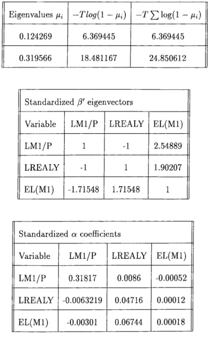
Table 11; Results of multicointegratiori analysis for M2 under the unit income elaticity restriction

Eigenvalues fii -T lo g {l - fii) _{- î " E l o g ( l}

0.124269 6.369445 6.369445

0.319566 18.481167 24.850612

Standardized j3' eigenvectors

Variable L M l/P LREALY EL(M l)

L M l/P 1 -1 2.54889 LREALY -1 1 1.90207 E L(M l) -1.71548 1.71548 1 Standardized a coefficients Variable L M l/P LREALY E L(M l) L M l/P 0.31817 0.0086 -0.00052 LREALY -0.0063219 0.04716 0.00012 E L(M l) -0.00301 0.06744 0.00018 43

A p p e n d ix C

Table 12: Results of multicointegration analysis for M l under the hyphoteses that coefficient of real income is 1/2 and coefhcient of expected loss is -1/2

Eigenvalues -Tlog{\ - m) - T E i o g i i - , . , )

0.120329 6.153948 6.153948

Standardized ¡¡)' eigenvectors

Variable L M l/P LREALY EL(M l)

L M l/P 1 -0.5 0.5 LREALY -2 1 -1 E L(M l) 2 -1 1 Standardized a coefficients Variable L M l/P LREALY E L(M l) L M l/P 0.17923 -0.0005321 0.0000866 LREALY 0.01940 -0.0000576 0.0000094 E L(M l) -0.06084 0.0001806 -0.0000294 44

Table 13; Results of rnulticointegration analysis for M2 under the hyphoteses that coefhcient of real income is 1/2 and coefficient of expected loss is -1/2

Eigenvalues -T lo g {i - gi) -TY^\og{\ - lii)

0.178967 9.465204 9.465204

Standardized ¡3' eigenvectors

Variable L M l/P LREALY EL(M l)

L M l/P 1 -0.5 0.5

LREALY -2 1 -1

E L(M l) 2 -1 1

Standardized a coefficients

Variable L M l/P LREALY EL(M l)

L M l/P 0.14396 -0.0005573 0.0001487

LREALY 0.02061 -0.0000798 0.0000213 E L(M l) -0.11334 0.0004387 -0.0001170

A p p e n d ix D

Table 14: Results of multicointegration analysis for M l under the hyphoteses that q;2 = 0

Eigenvalues ¡li -T lo g {i - fii) - T X ; i o g ( l - //¿)

0.075659 3.776361 3.776361

0.217166 11.752051 15.528412

Standardized /?' eigenvectors

Variable L M l/P LREALY EL(M l)

L M l/P 1 -2.27122 0.22121

LREALY -0.35527 1 -1.17632

E L(M l) -0.31402 5.32695 1

Standardized a coefficients

Variable L M l/P LREALY EL(M l)

L M l/P 0.37124 -0.15768 -0.0015286

LREALY 0 0 0

E L(M l) -0.12187 -0.24786 0.0024103

Table 15: Results of multicointegration analysis for M l under the hyphoteses that « 3 = 0

Eigenvalues fii - T % ( l - / . 0 - T ^ l o g { l - Hi)

0.091236 4.592160 4.592160 0.540173 37.291481 41.883641 Standardized ¡3' eigenvectors Variable L M l/P LREALY E L(M l) L M l/P 1 -3.26059 0.69336 LREALY -6.44721 1 -3.53183 E L(M l) 0.13822 -0.24843 1 Standardized a coefficients

Variable L M l/P LREALY EL(M l) L M l/P -0.01446 -0.02529 -0.0041311

LREALY -0.66519 -0.01234 0.00958

E L(M l) 0 0 0

Table 16: Results of multicointegration analysis for M l under the hyphoteses that a<2 = 0C3 = 0

Eigenvalues ¡xi -Tlog{\ - Hi) _{- 2 ' E l o g ( l - № )}

0.191334 10.1937 10.1937 Standardized eigenvectors Variable L M l/P LREALY E L(M l) L M l/P 1 -2.34674 0.65053 LREALY -0.11384 1 -0.27720 E L(M l) 0.12072 -0.03261 1 Standardized a coefficients

Variable L M l/P LREALY EL(M l)

L M l/P 0.42604 -0.0050732 -0.0065235

LREALY 0 0 0

E L(M l) 0 0 0

Table 17: Results of multicointegration analysis for M2 under the hyphoteses that « 2 = 0 Eigenvalues ¡Xi -T lo g {l - m) - r ^ l o g ( l - m) 0.131831 6.785716 6.785716 0.319938 18.507416 25.293132 Standardized ¡5' eigenvectors

Variable L M l/P LREALY EL(M l)

L M l/P 1 -0.89862 2.55311

LREALY 0.26849 1 -1.59184

EL(M l) 1.03967 -4.63742 1

Standardized a coefficients

Variable L M l/P LREALY EL(M l)

L M l/P 0.31399 0.0034527 0.004004

LREALY 0 0 0

E L(M l) -0.0061214 -0.12486 0.0042168

Table 18: Results of rnulticoiiitegration analysis for M2 under the hyphoteses that 0^3 = 0

Eigenvalues Hi -Tlog{\ - m)

_{-rEioe(i-/'.■ )}

0.319103 18.448554 18.448554

0.384789 23.317947 41.766501

Standardized eigenvectors

Variable L M l/P LREALY EL(M l)

L M l/P 1 -6.24356 1.17835

LREALY -0.85808 1 -2.15271

EL(M l) -0.36294 -0.06535 1

Standardized a coefficients

Variable L M l/P LREALY EL(M l) L M l/P -0.07113 -0.36735 0.0079036 LREALY -0.23931 0.06695 0.0053095

E L(M l) 0 0 0

Table 19; Results of multicointegration analysis for M2 under the hyphoteses that « 2 = Q!3 = 0

Eigenvalues /Xi -Tlog{\ - Hi)

0.319848 18.50105 18.50105

Standardized ¡3' eigenvectors

Variable L M l/P LREALY EL(M l)

L M l/P 1 -0.9108 2.57545

LREALY 0.77619 1 -2.82770

E L(M l) 0.81667 -3.91049 1

Standardized a coefficients

Variable L M l/P LREALY EL(M l) L M l/P 0.31284 -0.0020447 0.0051596

LREALY 0 0 0

E L(M l) 0 0 0