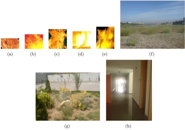
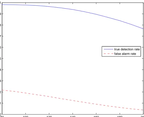
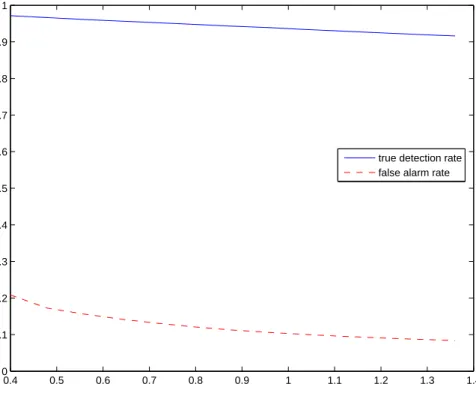
Fire and flame detection methods in images and videos
Tam metin
Şekil


Benzer Belgeler
Keywords: Lebesgue Constants, Cantor type Sets, Faber Basis, Lagrange Inter-
A “new” national architectural language expected to embody values and ideals of the brand new Kyrgyz nation, and at the same time to herald the construction of the strong tradition
The present study built on this approach by (a) investigating whether the distinction between autonomous or volitional and controlling or pressuring reasons can be mean-
Böylece erek dizge içerisinde Can Yücel’in Hamlet çevirisi “oynanamaz” ilan edilse bile, bu durum erek metnin kabul edilebilir bir çeviri olduğu ve istenildiğinde—belki
The general synthetic method described above afforded 5a, and the product obtained was in white crystalline solid form from 1-(4-chlorobenzhydryl)piperazine (1.98 mmol)
In this regard, the ability of CB[8] to form ternary complexes with suitably sized and functionalized guests have been extensively explored in the preparation of
Therefore, in the procedure of fiscal decentralization, equalization across local governments leads to higher size of redistribution but lower fiscal discipline compared
We aimed to develop an articulated figure animation system that creates movements , like goal-directed motion and walking by using motion control techniques at different
