Fiscal decentralization and fiscal discipline

FISCAL DECENTRALIZATION AND FISCAL DISCIPLINE A Master’s Thesis by NİDA ÇAKIR Department of Economics Bilkent University Ankara September 2006

FISCAL DECENTRALIZATION AND FISCAL DISCIPLINE

The Institute of Economics and Social Sciences of

Bilkent University

by NİDA ÇAKIR

In Partial Fulfillment of the Requirements for the Degree of

MASTER OF ECONOMICS

in

THE DEPARTMENT OF ECONOMICS BILKENT UNIVERSITY

ANKARA

I certify that I have read this thesis and have found that it is fully adequate, in scope and in quality, as a thesis for the degree of Master of Arts in Economics

--- Assist. Prof. Bilin Neyaptı Supervisor

I certify that I have read this thesis and have found that it is fully adequate, in scope and in quality, as a thesis for the degree of Master of Arts in Economics

---

Assist. Prof. H. Çağrı Sağlam Examining Committee Member

I certify that I have read this thesis and have found that it is fully adequate, in scope and in quality, as a thesis for the degree of Master of Arts in Economics

--- Assist. Prof. Zeynep Önder Examining Committee Member

Approval of the Institute of Economics and Social Sciences

--- Prof. Erdal Erel Director

ABSTRACT

FISCAL DECENTRALIZATION AND FISCAL DISCIPLINE Çakır, Nida

Master of Economics

Supervisor: Assist. Prof. Bilin Neyaptı September 2006

In this thesis, the effects of fiscal procedures, fiscal centralization and fiscal decentralization, on fiscal discipline are analyzed in a theoretical framework. A model of two optimization problems is established: central government’s optimization problem and local government’s optimization problem representing the two fiscal procedures; fiscal centralization and fiscal decentralization respectively. Comparative static analysis is performed, and moreover ambiguous results are calibrated. Our results indicate that in fiscal decentralization fiscal discipline increases with the number of localities. Furthermore, the portion that goes to the pool of the central government has a positive effect on the size of redistribution in fiscal centralization, but it has a negative effect in fiscal

decentralization. Similarly, whereas income tax rate affects the size of redistribution positively in fiscal centralization, it has a negative effect in fiscal decentralization. Keywords: Fiscal Decentralization, Fiscal Discipline

ÖZET

MALİ YERELLEŞME VE MALİ DİSİPLİN Çakır, Nida

Yüksek Lisans, İktisat Bölümü Tez Danışmanı: Yrd. Doç. Dr. Bilin Neyaptı

Eylül 2006

Bu tezde, mali usullerin, mali yerelleşme ve merkezileşme, mali disiplin üzerine etkileri teorik bir çerçevede incelenmiştir. Mali yerelleşme ve merkezileşmeyi sırasıyla temsil eden yerel hükümet eniyileme ve merkezi hükümet eniyileme problemlerini içeren bir model kurulmuştur. Karşılaştırmalı statik yapılmış ve ayrıca belirsiz sonuçlar kalibre edilmiştir. Sonuçlara göre, mali yerelleşmede, yerel hükümetlerin sayısı arttıkça mali disiplin artmıştır. Buna ilaveten, merkezi hükümetin havuzuna giden oran arttıkça, mali merkezileşmede toplam transfer miktarı artarken, mali yerelleşmede toplam transfer miktarı oran artışıyla azalmıştır. Benzer şekilde, mali merkezileşmede gelir vergisi oranı toplam transferler üzerinde pozitif bir etki yaratırken, mali yerelleşmede bu oran toplam transferler üzerinde negatif bir etki yaratmıştır.

Anahtar Kelimeler: Mali Yerelleşme, Mali Disiplin

ACKNOWLEDGEMENTS

I would like to thank to Prof. Bilin Neyaptı for her supervision and guidance through the development of this thesis.

I am indebted to Prof. H. Çağrı Sağlam who had spared his time to teach and encourage me, and thank to for his invaluable comments.

I would like to thank to Prof. Serdar Sayan, Prof. Neil Arnwine, and Prof. Tarık Kara for their support and comments.

I especially would like to express my deepest gratitude to Yusuf Işık, who introduced the world of economics to me and always encourages me, for his invaluable guidance in my last four years.

Finally, I owe special thanks to my mother, father, and my twin who have always supported my studies from the beginning.

TABLE OF CONTENTS ABSTRACT……….i ÖZET………..iii ACKNOWLEDGEMENTS……….v TABLE OF CONTENTS………vi LIST OF TABLES………..vii CHAPTER 1: INTRODUCTION ………1

CHAPTER 2: LITERATURE SURVEY………..7

CHAPTER 3: MODEL………19

3.1 Variables and Description of the Model………..22

3.2 Local Government’s Problem………..25

3.3 Central Government’s Problem………...28

CHAPTER 4: COMPARATIVE STATIC ANALYSIS……….32

4.1 Comparative Statics for the LG problem……….33

4.2 Comparative Statics for the CG problem………40

CHAPTER 5: CALIBRATION ANALYSIS………..46

5.1 Evaluation of the LG problem……….49

5.2 Evaluation of the CG problem……….62

5.3 Comparison of the Fiscal Procedures………..71

CHAPTER 6: CONCLUSION………74

APPENDIX……….76

BIBLIOGRAPHY………...78

LIST OF TABLES

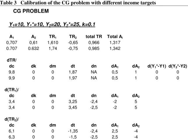
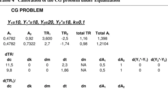
1. Table 1 Calibration of the LG problem with Different Income Targets....53 2. Table 2 Calibration of the LG problem under Equalization………..59 3. Table 3 Calibration of the CG problem with Different Income Targets...66 4. Table 4 Calibration of the CG problem under Equalization……….69

CHAPTER 1

INTRODUCTION

Government deficits are a matter of concern in most of the countries, developing or developed, for which reducing budget deficits by means of achieving fiscal discipline is an important phenomenon. Accordingly, in recent years, a growing number of countries around the world have increased efforts to improve on fiscal organizations, where fiscal decentralization (FD) is one aspect of these organizations.

Main issues that fiscal organizations or arrangements take into account are as follows:

i. How should the central and local government relationships be established? ii. Does the transfer system create negative incentives for localities to collect

taxes?

iii. How should intergovernmental transfers be structured so as to ensure fiscal discipline?

It can be deducted from the above questions that the structure of transfer systems is crucial, and the decisions of governments should be in such a way that they are able to reduce fiscal indiscipline, and income disparities.

An important aspect of fiscal arrangements, fiscal decentralization refers to devolution of revenue sources and expenditure functions to lower tiers of government. Accountability and transparency in government actions, streamlining public sector activities and encouraging the development of local democratic traditions (De Mello, 2000) carry important implications for the success of FD. Since the main goal of FD is to achieve lower budget deficits, the effect of fiscal decentralization on fiscal discipline is important.

There is a growing recent theoretical literature on fiscal arrangements and fiscal discipline, as well as optimal equalization grants. For instance, Von Hagen and Harden (1995) examine decision making procedures and fiscal discipline in a game theoretical framework. They take into consideration the budgeting procedures within the central government concerning the collective interest of the government and individual interest of spending ministers (SMs), and conclude that procedure oriented approach, that is the decision of SMs, leads to lower fiscal discipline.

Neyaptı (2006, forthcoming) addresses fiscal discipline via fiscal decentralization by means of extending the model of Von Hagen and Harden (1995) such that the effects of monetary discipline on budgetary outcomes can be examined. Unlike Von Hagen and Harden (1995) would predict, Neyaptı shows that, due to the addition of central bank independence feature into the model, one can obtain the result that as the number of SMs increases, total spending and deficits may decrease. Moreover, the higher the utility obtained from SMs’ individual spending, the higher are the spending biases and budget deficits.

In an analysis of the effects of different intergovernmental regimes on fiscal discipline, Sanguinetti and Tommasi (2004) argue that fiscal indiscipline

results from the optimization problem of the locality under incomplete information. Slightly different from the above studies, Dahlby and Wilson (1994) focus on

equalization grants in the context of optimal tax theory. Optimal equalization grants are formulated so as to distribute the tax burden across localities, and the authors conclude that when the share of total expenditures of a locality exceeds the share of total capacity, it is a recipient of grant.

This study offers a theoretical framework where we focus on the effects of fiscal procedures, i.e. fiscal decentralization and centralization, on fiscal

discipline1. In a way, we compare the fiscal procedures with regards to fiscal discipline. In doing this we also address the issue of equalization, where we construct the fiscal procedures of fiscal centralization and fiscal decentralization as the optimization problems of the central government and local government, respectively. The set up of our model includes a redistribution mechanism that depends on the tax effort and the deviation of the actual income from the target income of a locality. Moreover, fiscal discipline is measured via tax efforts resulting from the optimization problems. Hence, while focusing mainly on fiscal discipline by means of fiscal procedures; we address equalization and total transfers, i.e. size of redistribution, under a redistribution mechanism. The equalization concept here is referred to as the setting of target incomes across localities at the same level.

Different from the mentioned literature, fiscal procedures described in the current model, which yields the optimal tax effort and optimal transfers, are constrained by a redistribution mechanism which includes a measure of fiscal discipline as well as equalization. While maximizing the welfare of the society, a block mechanism preventing overspending of jurisdictions is formed. As a result,

our study focuses on the issues i to iii mentioned above. Main findings of our analysis are as follows:

i. In fiscal decentralization procedure, the number of localities is positively associated with fiscal discipline.

ii. In the procedure of fiscal decentralization, an increase in the deviation of actual output from its target creates a disincentive for a locality to increase its tax effort due to increase in transfers via this deviation of income.

iii. In the procedure of fiscal decentralization, the portion that goes to the pool of the central government has a negative effect on the size of redistribution, however in fiscal centralization a positive effect is observed.

iv. The income tax rate has a positive effect on the size of redistribution in fiscal centralization, but in fiscal decentralization it affects the size of redistribution negatively.

The remaining part of the study is organized as follows. Chapter 2 presents a literature survey on fiscal arrangements and fiscal discipline as well as equalization. Chapter 3 presents our model and solutions of our optimization

problems. Chapter 4 provides comparative static analysis. Chapter 5 submits the calibrated results obtained in the chapters 3 and 4. Finally, Chapter 6 concludes.

CHAPTER 2

LITERATURE SURVEY

Provision of economic efficiency and macroeconomic stability are among the main concerns of the governments. In this context, fiscal arrangements are crucial. The range of fiscal activities subject to such fiscal organizations includes the decisions on taxes, intergovernmental transfers, and debt financing, all of which have attracted a good deal of attention in the literature. Fiscal decentralization is one aspect of fiscal arrangement that the literature has widely focused on.

Many empirical studies have recently examined the advantages and or the pitfalls of fiscal decentralization. De Mello (2000) states that local governments meet local preferences and needs better than national governments. Since local

governments are much closer to the people and so more identified with local causes, information on the local preferences and needs costs cheaper reducing transaction costs. Hence, fiscal decentralization (FD) is expected to boost public sector efficiency, accountability, and transparency. But, on the other hand, De Mello (2000) also emphasizes that fiscal relations is a crucial and rather complex issue in decentralization, and failures in coordination of intergovernmental relations can result in a deficit bias, especially in the case of developing countries. It has been expressed that possible higher coordination and information costs to jurisdictions may prevent the realization of benefits of decentralization, and hence expenditure decentralization may worsen the situation.

Fiscal decentralization has two aspects: expenditure and revenue-collection decentralization of the governments. Decentralization of spending may increase economic efficiency which may imply lower deficits, but an increase in deficits is also possible. Within this frame, Neyaptı (2006) analyzes the relationship between budget deficits and fiscal decentralization using panel data techniques. Whereas expenditure decentralization is observed to be significant for deficits, revenue decentralization is not. The analysis focuses on various factors that are suggested to affect the relationship between FD and deficits by the literature. The

factors are as follows: the size of the government, business cycles, governance, size of the country, the presence of local elections, and the extent of ethno linguistic fractionalization.

Related to the factors that are analyzed by Neyaptı (2006), Davoodi (1998) shows the negative impact of FD on growth for developing countries based on the argument that the efficiency gains from FD may not materialize for developing countries since revenue collection and expenditure decisions by local governments may still be constrained by the central government.2 Similarly, Zou and Jin (2002) examine the effects of decentralization on government size. They conclude that expenditure decentralization leads to larger aggregate and sub national governments. However, revenue decentralization leads to larger sub national governments but it reduces national government’s size by more than it increases sub national governments’ sizes, and hence leads to a smaller aggregate government size.

There are also theoretical studies inspecting the structure of procedures for choices of the federal government and its jurisdictions, and the structure of transfer systems. Within this context, Sanguinetti and Tommasi (2004) analyze the

2

effects of different regimes of intergovernmental transfers on fiscal discipline and welfare. Analogous to our model, the model of Sanguinetti and Tommasi (2004) enables us to observe whether certain institutional arrangements weaken fiscal discipline or not. Furthermore, the paper determines the level of transfers in different institutional settings, and different from us, the authors consider the role of transfers on smoothing shocks to local incomes. Federal transfers are used as a risk sharing mechanism, and they finance expenditures of localities via stochastic income by the federal government. In the paper, in one regime, local income in each region is realized by the federal government, and via the optimization problem the federal government precommits to a certain level of transfers (called as the first best case). The set up is similar to the central government’s optimization problem in our model. While transfers compensate for both horizontal and vertical imbalances in Sanguinetti and Tommasi (2004), transfers compensate only for horizontal imbalances in our case and there is no ex-ante insurance. In our set up, central government does not collect taxes, localities collect taxes and a portion of the collection goes to the pool of the central government.

Sanguinetti and Tommasi (2004) study also incomplete information with two cases: commitment and Nash. In the commitment case, federal government

commits to a certain level of transfers knowing just the distribution of shocks, not the realization. In the latter, each locality maximizes its utility similar to the local government’s optimization problem in our model. They conclude that transfers and private consumption are higher than the first best case. Hence, incomplete information yields excessive sub-national spending. In this context, the effort related compensation mechanism which works as a punishment mechanism in the redistribution rule of transfers in our model may be considered as a block mechanism that prevents overspending.

Another important finding, which is also related to our analysis, of Sanguinetti and Tommasi (2004) is that in the Nash solution too little tax effort is observed when the resources of the federal government are not fixed and distortionary taxation is considered. Similarly, in our set up, under same income targets across two localities, the local government’s optimization problem yields lower total tax efforts than that of the central government implying lower fiscal discipline.

Dahlby and Wilson (1994) also elaborate equalization grants but in the framework of optimal tax theory. As in Sanguinetti and Tommasi (2004), they minimize the social cost of providing government services, which is equivalent to

maximizing the welfare of the society, where they relate equalization grants to tax effort and fiscal capacity. A similar relation is invigilated in our analysis that focuses on the distribution of tax burden across localities, where the grants are made. Even though the distribution of transfers according to a rule maximizing the welfare of the society is an analogous concept, we do not study optimal taxation. Differently, we focus on the fiscal procedures (centralization versus decentralization), where the decision of optimal tax effort that maximizes the welfare is made by the locality.

In Dahlby and Wilson (1994), an optimal equalization grant formula is examined which has expenditure and fiscal capacity mechanisms, and the equalization payments sum up to zero. This implies that the federal government takes from one locality and gives it to the other. Our redistribution rule of transfers similarly includes tax effort and income compensation mechanisms; however, all the collection is allocated back to the jurisdictions, so that they do not sum up to zero. Moreover, Dahlby and Wilson (1994) construct the formula such that if the share of total expenditures of a locality exceeds the share of total fiscal capacity, it

is a recipient of grant; which can be sighted in our analysis as we compensate a locality for lower actual income than the target income3.

While Dahlby and Wilson (1994) focus on how the tax burden in a federation should be distributed across jurisdictions so that equalization of the social marginal cost of raising revenue across localities via optimal grants is satisfied, Sanguinetti and Tommasi (2004) focus on different fiscal regimes of intergovernmental transfers and fiscal discipline. We, on the other hand, present a model that unify some aspects of both Sanguinetti & Tommasi (2004) and Dahlby & Wilson (1994) such that we elaborate both different fiscal procedures and optimal grants in a framework that allows us to address fiscal decentralization and fiscal discipline, as well as equalization.

Similar to Sanguinetti & Tommasi (2004), Von Hagen and Harden (1995) analyze how decision making procedures can be used as devices for fiscal discipline and affect fiscal performance of a government. The authors analyze fiscal discipline under a different set up, however. They consider the budgeting procedures within the central government describing different fiscal procedures concerning the collective interest of the government and individual interest of

3

Another equalization grant mechanism based on population is also considered by the authors. But, this does not yield optimal values and it is deducted that the resulting grants may reduce welfare.

spending ministers (SMs). Moreover, the paper focuses on fiscal illusion that is described as the overestimation of the marginal benefit of a public activity. The optimization problem of the government yields smaller optimal budget than the resulting budget of the SMs’ optimization problem implying a spending bias due to fiscal illusion. Lower spending bias can be interpreted as ensuring fiscal discipline. Within this context, we can conclude that fiscal decentralization results in fiscal indiscipline in Von Hagen and Harden (1995), which is parallel to our finding considering FD and fiscal discipline under equalization in a slightly different model. Similarly, Sanguinetti & Tommasi (2004) concludes that, under incomplete information, excessive sub national spending is observed. But, additionally, Von Hagen and Harden (1995) examine the case where SMs negotiate over the allocations, and a smaller optimal budget is obtained. So, they conclude that bargaining reduces the spending bias; which is equalization that reduces fiscal indiscipline in fiscal decentralization of our analysis. As a result, Von Hagen and Harden (1995) state that strengthening the collective interest the government can reduce the spending bias, which could be achieved via vesting the ministers without portfolio with special strategic powers. Modeling this approach indicates that when the ministers without portfolio have little strategic power, the optimal budget gets

closer to the bargaining optimal budget of the SMs. However, when they have full strategic power, the collective optimal budget is reached. Hence, the paper observes a positive relation between spending bias and the relative strength of SMs’ individual incentives against collective interest of the government.

A unifying theme of Von Hagen & Harden (1995) and Neyaptı (2006) is fiscal discipline which is addressed via budgeting procedures in the former and fiscal decentralization in the latter. Moreover, Neyaptı (2006, forthcoming) extends the model of Von Hagen & Harden (1995) such that the effects of not only fiscal discipline but also monetary discipline on budgetary outcomes can be inspected. Neyaptı (2006, forthcoming) incorporates central bank independence (CBI) as a measure of monetary discipline and a budget constraint into the model of Von Hagen & Harden (1995). Different from Von Hagen & Harden (1995), deficits are financed through money issue inversely related with the degree of CBI and through bond issue, and all monetary expansion is inflationary. Moreover, model predictions are tested empirically for 12 OECD countries during the 1980s. The results support the model results. The results are such that if the central bank is totally independent, all SMs’ spending are on target and inflation is zero. Otherwise, there is a negative relationship between the deviations of spending and inflation from their respective

targets. When the central bank is not totally independent, Nash bargaining solution leads to lower spending bias than the individual optimization of SMs.

Consistent with Von Hagen & Harden (1995), Neyaptı (2006, forthcoming) observes that the government’s collective interest yields lower budget deficits, and lower inflation rates than the SMs’ individual and Nash bargaining solutions. She also states that the lack of monetary discipline increases fiscal discipline on the part of spending ministers, since the model imposes that they internalize the cost of their spending. Hence, as the number of the SMs (

n

) increases, the government may cut back on total spending and deficits due to the expectation that both total spending and inflation would increase. Two other important findings of Neyaptı (2006, forthcoming) are as follows: the first is that as

n

increases, the spending bias that arises from Nash bargaining solution increases as compared to that of the government’s collective interest. That is, increase in the number of localities leads to lower fiscal discipline in the Nash bargaining case than the government’s collective interest. The second is that the higher the utility received from individual SMs’ spending, the higher are the spending biases and budget deficits, implying lower fiscal discipline. Even though, we can not do a comparison between our procedures with respect to a change in

n

, in our model, as

the number of localities increases, higher fiscal discipline is provided under fiscal decentralization. Contrary to the second finding, calibration analysis of fiscal decentralization procedure concludes that the higher the utility obtained from government expenditures the higher the fiscal discipline.

Neyaptı (2005) examines fiscal decentralization under a different set up from the above theoretical studies. Like Dahlby and Wilson (1994), the paper focuses on equalization but, in the frame of fiscal decentralization using regression analysis considering the provinces of Turkey. In the paper, in addition to the main concerns for FD, main issues that affect the success of FD are mentioned. It is stated that equality, macroeconomic stability, and economic efficiency are among the main issues of FD. Eliminating vertical imbalances along with reducing horizontal imbalances is the “equalization” concept of the paper. Moreover, the paper realizes equalization feature as a disciplining device in case of FD. Our model considers equalization as an additional crucial issue to be analyzed along with the fiscal procedure of decentralization, while focusing mainly on the provision of fiscal discipline. Similar to Dahlby and Wilson (1994) and our study, the paper proposes a redistribution method for Turkey based on the measures of vertical and horizontal imbalances across the jurisdictions, where our redistribution mechanism

only considers horizontal imbalances based on a theoretical set up. As also told by Dahlby and Wilson (1994), Neyaptı (2005) states that focusing only on a population based system of distribution of the revenue pool is not meaningful. An egalitarian redistribution system can be better. Then, she concludes that the better the macroeconomic performance, the larger the municipal revenues, and the better the socio-economic status, the larger the municipal spending. In addition, the paper deducts that a reasonable system of redistribution should be based on socio-economic characteristics.

In summary, fiscal decentralization has important implications for economic efficiency. While FD can be promoted due to provision of more identified local causes and cheaper costs of information on the local preferences and needs, it can also lead to excessive sub national spending, high budget deficits, lower tax efforts, and so lower fiscal discipline. Hence, exploring the design of fiscal decentralization along with its impact on fiscal discipline and equalization still remains to be an important issue.

CHAPTER 3

MODEL

Consider an economy where there are n local governments and a central government. Governments’ main objective is to maximize the welfare of the society. The central government (CG) collects taxes from each locality. “c” proportion, where

0

< <

c

1

, of all collected taxes goes to the pool of the central government, all of which is then allocated back to the regions as transfers. Moreover, we assume that only local governments undertake government spending in a locality and CG has no spending.

Local governments (LGs) collect effective income taxes and make expenditures that are financed by part of the tax collection that does not go to the pool of the CG (c portion of the tax collection goes to the pool) plus the transfers. Allocation of transfers to each locality is based on a redistribution rule which is composed of a punishment mechanism and an income compensation mechanism. The punishment mechanism depends on the deviation of tax effort of the locality

from the target value “1”, and the income compensation mechanism refers to the transfers compensation based on the deviation of actual output of the locality from its target output. In our model, the deviations of actual output of the localities from their target output indicate horizontal imbalances. As this deviation increases, imbalance grows. Hence, to be able to compensate the imbalance, transfers should rise. Therefore, one part of the redistribution rule works as an income compensation mechanism. So, the tax effort of the locality and the deviation of actual output from the target are crucial for the transfers a locality receives.

We are going to analyze two fiscal procedures represented by the central government’s and the local governments’ optimization problems4. CG decides on the level of transfers allocated to each locality while maximizing the overall welfare of the society subject to the collection constraint. The optimization problem of CG is referred to as “fiscal centralization”. On the other hand, LG maximizes the welfare of its jurisdiction subject to the redistribution rule and decides on the level of its tax effort. We refer to LG’s optimization as “fiscal decentralization”.

Tax effort level is important in analyzing fiscal discipline. We characterize “fiscal discipline” in each problem as the total of tax efforts across the

4

We also studied the problems when either CG or LG is the leader. Because of the set ups of the CG and LG problems (and their constraints), the leader problems do not give meaningful results. So,

local governments. Furthermore, the optimal level of total transfers is characterized as “the size of redistribution” in each problem. The main objective of studying these two procedures is to be able to answer the question: “Does fiscal decentralization cause more fiscal discipline?”. Hence, we aim to evaluate the two different fiscal procedures (CG and LG problems that represent fiscal centralization and decentralization respectively) on the basis of fiscal discipline they lead to; that is we compare the two problems vis a vis both fiscal discipline and also the size of redistribution. Therefore, the evaluation of our results depends on total tax efforts and total transfers implied by the two problems. Based on these results, comparative static analyses are utilized in the next chapter for studying the effects of the main parameters of the model on fiscal discipline and the size of redistribution.

In the following section, first we describe the common expressions and variables of the two problems. Then, we study the problems and solutions separately in sections 3.2 and 3.3.

3.1 Variables and Description of the Model

The effective tax rate of the Central Government is defined as

t

_i

=

tA

_i

where

t

is the exogenous common income tax rate and

A

_i is the tax effort of the ith locality, where

0

< <

t

1

and

0

<

A

_i

≤

1

5

.

Y

i

=

f K L

(

i

,

i

)

is the per capita production of locality i (actual output),

which is exogenous with given

,

i i

K L

per capita capital and per capita labor amounts for each locality6.

T

_i

=

t Y

_{i i} is the effective income tax of region i.

1 n i i

c

T

=

∑

is the total revenue of the Central Government, where c is the proportion of effective local taxes that is given to CG7.

Y

_i*is the exogenously determined target level of output of locality i.

5

Distribution depends on local governments’ tax efforts and the deviation of actual output from target output. To avoid from corner solution (zero tax effort) in the LG problem and to create a redistribution mechanism, we limit the level of tax efforts as

0

<

A

_i

≤

1

where “1” is the target value.

6

All variables are in per capita terms.

7 ₀

n n

C

i

=

Y

i

−

T

i

=

(1

−

t Y

i

)

i

=

(1

−

tA Y

i

)

i is the private consumption which is

the after tax income, where we assume

C

i

>

1

. It is therefore observed that

C

i is a

decreasing function of

A

_i.

Local government expenditures are composed of transfers received from the central government

(

TR

_i

)

and the part of the effective income tax revenue that does not go to the pool of the central government. That is,

G

i

=

TR

i

+

(1

−

c t Y

)

i i is

the government expenditure of the ith locality. We also assume that

G

i

>

1

8 .

It can be observed that the market clearance condition is satisfied for the

CG problem: 1 1

(

)

n n i i i i i

Y

C

G

= =

=

+

∑

∑

. It is, however not the case for the LG problem, since

Y

_i

=

C

_i

+

G

_i does not necessarily hold so long as

TR

_i

≠

ctAY

_{i i}, meaning that transfers are not necessarily equal to locality’s contribution to the common pool Transfers are distributed according to the following redistribution mechanism that has both a punishment and a compensation components to achieve discipline and income equality:

8

In the following section, we construct the problems such that the governments get utility from private consumption and government expenditures, where the utility is a concave function of C_i and

i

G . Within this frame, to have well defined problems the specified assumptions, C_i>1 and G_i>1, are made.

*

(

)

(

)

i i i i

TR

=

k t

−

t

+

m Y

−

Y

(3.1)

where

k

is the “punishment parameter” or the effort related compensation parameter (

k

>

0

, a policy variable), and m is the “income compensation parameter” or the weight on the income compensation, where

0

<

m

<

1

. The first part of the rule,

kt A

(

i

−

1)

, works as a punishment mechanism such that the lower

the tax effort of the ith locality the lower the transfer given to it. Therefore, transfers are designed to generate incentives for localities to provide tax effort, since they are given according to provided tax effort. On the other hand, the second part,

*

(

i i

)

m Y

−

Y

, works as an income compensation mechanism such that the lower the deviation of actual output of the ith locality from target, the lower the transfers it receives so that equality across regions can be reached9. Hence, the central

9

In our model the target output of the ith locality is indicated by

Y

_i*and it is exogenous.

If

Y

_i*

=

Y

*for all i, the income compensation mechanism turns out to be an “equalization mechanism”. That is, setting all the targets at the same level is “equalization”.

Alternatively, the target output can be defined as

Y

_i*

=

g K L

(

_i

,

_i

)

and

Y

_i

=

Y

_i*

+

ε

_i, where

ε

_iis a random shock. We may also consider a production function that is the same for all localities, but there are different endowments and different shocks. If *

1

(

)

0

n i i i

Y

Y

=





−

>







∑



, then 1

0

n i i

ε

=





<







∑



government’s transfers are used for both income compensation and provision of fiscal discipline. From (3.1) one can observe that a locality can receive zero transfers when

A

_i is “1” and income is on target. Furthermore, the rule works completely as a punishment mechanism for a locality having a high level of output as compared to the target even if full tax effort (“1”) is provided. This is due to the fact that

Y

_i*

−

Y

_i decreases as

Y

_i increases, and CG can compensate the horizontal imbalances by means of transfers when the actual output of the locality is less than the target.

For both problems, preferences are defined over private consumption and government expenditures. The problems are discussed in detail in the following sections, 3.2 and 3.3.

3.2 Local Government’s Problem10

The utility function of the ith locality is defined as

ln

ln

i i i

U

=

α

C

+

β

G

(3.2)

We also consider the case where

Y

_i*

=

Y

, but it causes the income compensation part of the redistribution rule to disappear and the size of the redistribution to be non positive which contradicts with our model set up.

10

We study the problem of Local Government for an arbitrary locality because the problem is same for other localities.

where

U

_i is concave and increasing in both

C

_i and

G

_i, and 2

0

i i i

U

G C

∂

≥

∂ ∂

. Moreover, i

U

satisfies the Inada conditions. That is,

0

lim

i i C i

U

C

→

∂

= ∞

∂

and

lim

i 0 i G i

U

G

→

∂

= ∞

∂

.

(3.2) shows that a locality gets utility from private consumption and government expenditures in proportions of

α

,

0

<

α

<

1

, and

β

,

0

<

β

<

1

, respectively11.

The optimization problem of LG is defined as the maximization of the welfare of the locality subject to the redistribution mechanism:

i A

maximize

U

i

=

α

ln

C

i

+

β

ln

G

i (3.3) *

i

(

i

1)

(

i i

)

subject to TR

=

kt A

−

+

m Y

−

Y

(3.1)

To solve the problem, we first replace

C

_i by

(1

−

t Y

i

)

i and

G

i by

TR

i

+

(1

−

c t Y

)

i i

in (3.3), which yields: *

max ln((1-

) )

ln(

(1

)

)

.

(

1)

(

)

i i i i i i A i i i i

tA Y

TR

c tAY

s to TR

kt A

m Y

Y

α

+

β

+

−

=

−

+

−

11

In the following calibrations, we use the standard form of Cobb Douglas function such that

As can be observed, if transfers increases, government expenditures increases which in turn increases the utility.

Now, to convert the problem into an unconstrained optimization problem, we insert (3.1) into the objective function. Then, we have

*

max

( ln((1-

) )

ln( (

1)

(

)

(1

)

))

i

i i i i i i i i

A

V

=

α

tA Y

+

β

kt A

−

+

m Y

−

Y

+

−

c tAY

(3.4)

Our solution to this problem should satisfy the first order and second order optimality conditions. The first order condition of the problem is

*

( ln((1-

) )

ln( (

1)

(

)

(1

)

))

0

i i i i i i i i

tA Y

kt A

m Y

Y

c tA Y

A

α

β

∂

+

−

+

−

+

−

=

∂

(3.5) and it results in *

(

(

))

(

)(

(1

) )

(

)

o i i i i

kt

m Y

Y

A

t

k

c Y

t

α

β

α

β

α

β

−

−

=

+

+

+

−

+

(3.6)

A

_io characterizes the optimal

A

_i obtained as the solution of the problem if it also satisfies the second order optimality condition. The second order optimality

condition is described as 2 2

0

i i

V

A

∂

≤

∂

at o i

A

. 2 2 2 2 2 * 2

(

(1

)

)

(1

)

( (

1)

(1

)

(

))

i i i i i i i i i

V

t

kt

c tY

A

tA

kt A

c tA Y

m Y

Y

β

α

∂

+

−

= −

−

∂

−

−

+

−

+

−

(3.7)

When we evaluate (3.7) at

A

_io, we have the following: 2 2 3 * 2

(

(1

) ) (

)

0

( (

1)

(

1)

)

i i i

t k

c Y

k t

c

m

Y

mY

α

β

αβ

+

−

+

−

≤

−

+

+

−

−

.

Hence, the second order optimality condition is also satisfied. Therefore,

A

_io is the optimal tax effort for the LG problem12.

From (3.6), we obtain the total optimal tax efforts of the LGs as:

* 1 1

(

(

))

(

)(

(1

) )

(

)

n n o i i i i i _i

kt

m Y

Y

A

t

k

c Y

t

α

β

α

β

α

β

= =



₋

₋



=



+



+

+

−

+





∑

∑

(3.8)

which is the expression for fiscal discipline in fiscal decentralization. Given (3.1), we also observe that

* 1 1

( (

1)

(

))

n n i i i i i i

TR

kt A

m Y

Y

= =

=

−

+

−

∑

∑

(3.9)

Inserting (3.6) into (3.9) results in

* * 1 1 1

(

)

(

)

(1

)

n n n i i i i i i i i _i

kt

m Y

Y

k

TR

TR

m Y

Y

nk

t

k

c Y

α

β

α

β

α

β

= = =



₋

₋







=

=

−

+





+



−



+



+

−





+



∑

∑

∑

(3.10

) Therefore, (3.10) is the optimal size of redistribution for the LG problem.

3.3 Central Government’s Problem

The utility function of CG

( )

U

is defined as the sum of the utilities of all regions: 1 1

( ln

ln

)

n n i i i i i

U

U

α

C

β

G

= =

=

∑

=

∑

+

(3.11)

The optimization problem of CG is

TRi ₁

max imize

( ln

ln

)

n i i i

C

G

α

β

=

+

∑

(3.12) subject to 1 1

(

)

n n i i i i i

TR

ctAY

= =

=

∑

∑

(3.13)

The problem specifies that overall welfare of the society is to be maximized while

all the taxes collected,

1

(

n i i i

ctAY

=

∑

) >0, are distributed back to regions as transfers. Now, we proceed with the solution of the problem. The Lagrangean function is: 1 1 1

( ln

ln

)

(

)

n n n i i i i i i i i

L

α

C

β

G

λ

ctAY

TR

= = =

=

∑

+

+

∑

−

∑

where

λ

is the Lagrange multiplier. The value of the Lagrange multiplier at the solution of the problem is equal to the rate of change in the maximal value of the objective function as the constraint is relaxed. As in LG problem we replace

C

_i by

(1

−

t Y

i

)

i and

G

i by

TR

i

+

(1

−

c t Y

)

i i, and obtain the first order conditions as:

0

(1

)

i i i i

L

TR

TR

c tAY

β

λ

∂

=

−

=

∂

+

−

(3.14) 1 1

0

n n i i i i i

L

ctAY

TR

λ

= =

∂

=

−

=

∂

∑

∑

(3.15)

Combining (3.14) and (3.15) yields:

1

(1

)

n o i i i i i i

t

TR

AY

c tAY

n

=





=





−

−



∑



(3.16)

(3.16) should also satisfy the second order necessary conditions to be the optimal solution to the CG problem.

To examine the 2nd order necessary conditions, we are going to check

the rank of 1 1

0

i n n TR i i i i i

TR

ctAY

= =





∂



−

=





∑

∑



, and second order derivative of the

( )

1 1

0

1

1

i n n TR i i i i i

Rank

TR

ctAY

Rank

= =









∂



−

=



=

=











∑

∑



. Moreover,

( )

2 2

0

((1

)

)

i TR i i i

L

c t Y

TR

β

−

∂

=

<

−

+

at o i

TR

. Hence, the rank equals to the number

of constraints and second order derivative of the Lagrangean function is negative implying that the second order optimality condition is met. Therefore, (3.16) is the optimal solution to the CG problem. According to (3.16), one can observe that transfer distribution of the central government depends basically on the tax effort and actual income of jurisdiction. Moreover, the total size of redistribution of the problem is given by:

1 1 1 1

(1

)

n n n n i i i i i i i i i i i

t

TR

TR

AY

c tAY

ct

AY

n

= = = =









=

=







−

−



=









∑

∑

∑

∑

.

In the next chapter, we do comparative static analysis for

A

_i,

TR

_i, and

CHAPTER 4

COMPARATIVE STATIC ANALYSIS

In order to examine the relationship between fiscal decentralization and fiscal discipline we need to perform comparative static analysis. To this end, we are going to study partial derivatives of the size of redistribution, optimal level of transfers and tax effort with respect to:

*

, , , , , , , (

_{i i}

)

c k m t n

α β

Y

−

Y

for both the CG and the LG problems. In addition, we will inspect how transfers change with respect to a change in the tax effort. We think that this analysis will enable us to make judgements about the effectiveness of different fiscal procedures, where effectiveness is with respect to fiscal discipline and the elimination of horizontal imbalances.

4.1 Comparative Statics for LG problem

The effects of the specified variables on the optimal tax efforts and the size of redistribution are analyzed in the following subsections 4.1.1 and 4.1.2 respectively.

4.1.2 Partial Derivatives for Optimal Tax Effort

We use the expression that we have obtained in the LG problem:

*

(

(

))

(3.6)

(

)(

(1

) )

(

)

i i i i

kt

m Y

Y

A

t

k

c Y

t

α

β

α

β

α

β

−

−

=

+

+

+

−

+

i=1,.., n.

whose partial derivative with respect to the portion of taxes (c) that goes to the pool of the central government is:

* 2

((

(

))

(

) )

(

)(

)

(

) (

)

i i i i i i i i i i i

A

Y

Y kt

m Y

Y

k

Y

cY

c

t k

Y

cY

t k

Y

cY

β

α

β

α

β

α

β

∂

+

−

+

+

−

= −

+

∂

+

−

+

+

−

+

(4.1)

The sign of (4.1) cannot be determined. In cases of ambiguous signs, we utilize calibration analysis as will be reported in the next chapter.

Equation (4.2) shows how tax effort responds to a change in the effort related compensation parameter:

* 2

(

(

))

(

)

(

)(

)

(

) (

)

i i i i i i i i i

A

t

kt

m Y

Y

k

Y

cY

k

t k

Y

cY

t k

Y

cY

α

β

α

β

α

β

α

β

∂

+

+

−

+

+

−

=

−

∂

+

−

+

+

−

+

(4.2)

If

(

Y

i*

−

Y

i

)

>

0

, tax effort increases with the effort related compensation.

According to the redistribution rule, income compensation increases the transfers received. This creates an incentive for a locality to increase its tax effort via effort related compensation.

The partial with respect to the income compensation parameter yields:

*

(

)

(

)(

)

i i i i i

A

Y

Y

m

t

k

Y

cY

α

α

β

∂

−

=

∂

+

+

−

(4.3)

According to (4.3), if actual output is higher than the target, as the rate of income

related compensation increases tax effort of locality i increases. That is,

A

i

0

m

∂

>

∂

.

One explanation is that, TR will decrease if

Y

_i

>

Y

_i*. So, to be able to compensate this decrease in transfers, local government should increase its tax effort. On the other hand, if actual output is lower than the target, as m increases tax effort decreases. That is, TR will increase if

Y

_i

<

Y

_i* (income compensation mechanism). So, there will be no need to increase

A

_i for the locality to increase transfers. Therefore, high TR may create a disincentive for tax effort.

The effect of common income tax rate on tax effort is given by: * 2

(

(

))

(

)

(

)(

)

(

)(

)

i i i i i i i i i

A

k

kt

m Y

Y

k

Y

cY

t

t k

Y

cY

t k

Y

cY

α

β

α

α

β

α

β

∂

+

−

+

+

−

=

−

∂

+

−

+

+

−

+

(4.4)

Similarly, we are not able to observe the sign of (4.4). Calibration will tell us the sign.

As the deviation of the actual income from its target increases, tax effort of the ith locality decreases:

*

(

)

(

)(

)

i i i i i

A

m

Y

Y

t k

Y

cY

α

α

β

∂

= −

∂

−

+

−

+

(4.5)

This is due to increasing transfers via the increase in

(

Y

_i*

−

Y

_i

)

, which creates a disincentive for the locality to increase its tax effort.

The effect of the proportion of private consumption in utility on tax effort is also ambiguous:

* * 2

(

)

(

(

))

(

)

(

)(

)

(

)(

)

i i i i i i i i i i i

A

kt

m Y

Y

kt

m Y

Y

k

Y

cY

t k

Y

cY

t k

Y

cY

α

β

α

α

β

α

β

∂

+

−

+

−

+

+

−

=

−

∂

+

−

+

+

−

+

(4.6)

Similar to the above, the effect of the utility proportion of government expenditure on tax effort is ambiguous:

* 2

(

(

))

(

)

1

(

)

(

)(

)

i i i i i i i

A

kt

m Y

Y

k

Y

cY

t

t k

Y

cY

α

β

β

α

β

α

β

∂

+

−

+

+

−

=

−

∂

+

+

−

+

(4.7)

Calibration will show us the sign of these effects.

As we can observe from (3.6), we are not able to examine the effect of the number of jurisdictions on the optimal tax effort. However, we can observe the

effect of

n

on fiscal discipline, 1

0

(

n i i

A

n

t

β

α + β)

=





∂ 







=

>

∑

. Hence, the following

proposition arises:

Proposition 1: The number of the local governments has a positive effect on fiscal discipline.

A locality should provide tax effort to get transfers from the central government. Hence, an increase in number of localities may result in an increase in total tax efforts.

4.1.2. Partial Derivatives for the Size of Redistribution

Expression for the size of redistribution for LG problem from section 3 is: * * 1 1 1

(

)

(

)

(1

)

n n n i i i i i i i i

kt

m Y

Y

k

TR

TR

m Y

Y

nk

t

k

c Y

α

β

α

β

α

β

= = =



₋

₋







=

=

−

+





+



−



+



+

−





+



∑

∑

∑

(3.10)

The effect of the proportion that goes to the pool of CG on the size of redistribution depends on

(

*

)

1

(

)

n i i i i

Y Y

Y

=

−

∑

: * 2 1

( (

)

(

(

)))

(

)(

)

(

)(

)

n i i i i i i i _{i i i i}

Y

Y

k

Y

cY

kt

m Y

Y

TR

kt

c

t

k

Y

cY

t

k

Y

cY

β

β

α

α

β

α

β

=



₊

₋

₊

₊

₋



∂

=



−

+



∂

∑

_

+

+

−

+

+

−

_

(4.8) If

(

2 *

)

1

0

n i i i i

Y

Y Y

=

−

>

∑

, as c increases the size of redistribution increases.

Similarly, the effect of the punishment rate on the size of redistribution is uncertain: * 2 1 * 1

(

)

(

(

))

(

)(

)

(

)(

)

(

)

(

(

))

(

)(

)

n i i i i i _{i i i i} n i i i i i _{i i}

k

Y

cY

kt

m Y

Y

TR

t

nt

kt

k

t

k

Y

cY

t

k

Y

cY

k

Y

cY

kt

m Y

Y

t

t

k

Y

cY

β

α

α

β

α

β

α

β

β

α

α

β

= =



₊

₋

₊

₊

₋



∂

+

= −

+



−



+

∂

_

+

+

−

+

+

−

_



₊

₋

₊

₊

₋







+

+

−





∑

∑

(4.9)

The effect of income compensation rate on the size of redistribution is also ambiguous: * * 1 1

(

)

(

)

(

)(

)

n n i i i i i i _{i i}

Y

Y

TR

Y

Y

kt

m

t

k

Y

cY

α

α

β

= =



₋



∂

= −

−

+





∂

∑

∑



+

+

−



(4.10)