^ T E E D j::!
mBMlTTMS>· TOTEM m p A M T U E M T
MLMCT^JCAL-AH:^·
E L E C T R O m c s E m n U M F Jira
A^ND
t h e i n s t i t u t e o f£N€iNEMRiMG /ilfD
OF BILTMMT UNIVEMF'^^
ilfFA R T IA L FULFILL^FM^IT 0^^ TEE. MQUIFMIFM^^TJ
T k
7 8 9 2
• F SINVESTIGATIONS ON EFFICIENT ADAPTATION
ALGORITHMS
A THESIS
SUBMITTED TO THE DEPARTMENT OF ELECTRICAL AND ELECTRONICS ENGINEERING
AND THE INSTITUTE OF ENGINEERING AND SCIENCES OF BILKENT UNIVERSITY
IN PARTIAL FULFILLMENT OF THE REQUIREMENTS FOR THE DEGREE OF
MASTER OF SCIENCE
By
M urat Beige September 1995
τ κ - FS
ABSTRACT
IN V E S T IG A T IO N S O N E F F IC IE N T A D A P T A T IO N A L G O R IT H M S
Murat Beige
M .S . in Electrical and Electronics Engineering Supervisor: Assist. Prof. Dr. Orhan Arikan
September 1995
Efficient adaptation algorithms, which are intended to improve the perfor mances of the LMS and the RLS algorithms are introduced.
It is shown that nonlinear transformations of the input and the desired signals by a softlimiter improve the convergence speed of the LMS algorithm at no cost, with a small bias in the optimal filter coefficients. Also, the new algorithm can be used to filter a-stable non-Gaussian processes for which the conventional adaptive algorithms are useless.
In a second approach, a prewhitening filter is used to increase the con vergence speed of the LMS algorithm. It is shown that prewhitening does not change the relation between the input and the desired signals provided that the relation is a linear one. A low order adaptive prewhitening filter can provide significant speed up in the convergence.
Finally, adaptive filtering algorithms running on roughly quantized signals are proposed to decrease the number of multiplications in the LMS and the RLS algorithms. Although, they require significantly less computations their preformances are comparable to those of the conventional LMS and RLS algo rithms.
ÖZET
V E R İM L İ U Y A R L A M A A L G O R İT M A L A R IN IN A R A Ş T IR IL M A S I
Murat Belge
Elektrik ve Elektronik Mühendisliği Bölümü Yüksek Lisans Tez Yöneticisi: Dr. Orhan Arıkan
Eylül 1995
EOK (LMS) ve OEK (RLS) uyarlama algoritmalarının performanslarını geliştirmek amacıyla, verimli uyarlama algoritmaları tanıtılmıştır.
Giriş ve referans işaretlerinin doğrusal olmayan bir dönüşüm yolu ile yumuşak sınırlandırıcıdan geçirilmesinin, işlem karmaşıklığını arttırmadan en iyi süzgeç parametrelerinde küçük bir sapma ile, EOK algoritmasının yakınsama hızını arttırdığı gösterilmiştir. Yeni tanımlanan algoritma, birçok uyarlama algoritmasının çalışmadığı Gauss dağılımına sahip olmayan rastgele süreçlerin süzgeçlenmesinde kullanılabilir.
ikinci bir yaklaşımda, bir ön beyazlaştırıcı filtre EOK algoritmasının yakınsama hızının arttırılması amacıyla kullanılmıştır. On beyazlaştırıcı fil trenin giriş ve referans işaretleri arcisındaki lineer bir ilişkiyi değiştirmediği gösterilmiştir. Düşük dereceli bir ön beyazlaştırıcı filtre EOK algoritmasının yakınsama hızını önemli bir derecede arttırabilmektedir.
Sonuncu olarak, EOK ve OEK algoritmalarının hesap karmaşıklığının azaltılması için, kabaca seviyelendirilmiş işaretler üzerinde çalışan uyarlamalı süzgeç algoritmaları önerilmiştir. Bu algoritmalar, klasik EOK ve OEK algo ritmalarından çok daha az hesap gerektirmelerine rağmen performansları bu algoritmaların performansları ile kıyaslanabilir derecededir.
I certify that I have read this thesis and that in my opinion it is fully adequate, in scope and in quality, as a thesis for the degree of Master of Science.
S i . O i K j U ^
.Assist. Prof. Dr. Orhan Ankan(Supervisor)
I certify that I have read this thesis and that in my opinion it is fully adequate, in scope and in quality, cis a thesis for the degree of Master of Science.
A
Assoc. Prof. Dr. Enis Çetin
I certify that I have read this thesis and that in my opinion it is fully adequate, in scope and in quality, as a thesis for the degree of Master of Science.
V Assisk Prof. Dr. Billur Bdrshan
Approved for the Institute of Engineering and Sciences:
Prof. Dr. Mehme^^^Aray
ACKNOWLEDGEMENT
I would like to express my deep gratitude to my supervisor Dr. Orhan Arikan and Dr. Enis Çetin and Dr. Billur Barshan for their guidance, suggestions, and invaluable encouragement throughout the development of this thesis.
And special thanks to all Graduate Students in this department for their continuous support.
TABLE OF CONTENTS
1 INTRODUCTION
1
2 INVESTIGATION OF NONLINEAR PRE-FILTERING IN
LEAST MEAN SQUARE ADAPTATION
4
2.1 Introdu ction... 4
2.2 The LMS A lg o r it h m ... 5
2.2.1 Convergence In the Mean ... 6
2.2.2 Convergence In the Mean S q u a re... 7
2.3 The Nonlinear LMS Algorithm (NLMS) 8 2.4 Convergence A n a ly s is ... 12
2.5 Computer Sim ulation... ^ ... 19
2.6 Steady State Mean Square E rror... 20
2.7 Performance of NLMS Under Additive Impulsive Interference . . 22
2.7.1 Computer Sim ulation... 26
2.8 Adaptive Filtering Approaches for Non-Gaussian Stable Processes 27 2.8.1 Use of Pre-nonlinearity in Adaptive Filtering... 29
2.8.2 Computer S im u la tio n s... 30
2.9 C onclusion... 32
3 USE OF A PREWHITENING FILTER IN LMS ADAPTA
TION TO INCREASE CONVERGENCE SPEED
34
3.1 Introduction... 343.2 Proposed Adaptive A lg o r ith m ... 35
3.2.1 Determination of Whitening Filter C o e ffic ie n ts ... 37
3.4 Computational C o s t ... .39
3.5 Computer S im u la tion s... 10
3.6 C onclusion... 11
4 QUANTIZED RECURSIVE LEAST SQUARES ALGO
RITHM
44
4.1 I n tr o d u c tio n ... 444.2 Quantized Recursive Least Squares A lg o r it h m ... 45
4.2.1 Derivation ... 47
4.2.2 Computational Cost 50 4.2.3 Computer S im u la tio n ... 51
4.3 Fast Sequential Least Squares Adaptation Under Quantized Input and Desired S ig n a ls ... 53
4.3.1 Fast Algorithm Based On A Priori E rrors:... 56
4.3.2 Computational C o s t ... 59
4.4 Least Mean Square Adaptation Under Roughly Quantized In put and Desired Signals 60 4.4.1 Computational Cost ... 63
4.4.2 Computer S im u la tio n ... 64
4.5 C o n c lu s io n ... 64
4.6 A p p e n d ix ... 65
LIST OF FIGURES
2.1 Adaptive fUtering block diagram... 6 2.2 NLMS block diagram... 9 2.3 Variation of condition number as a function of clipping value of
the softlimiter. Upper curve corresponds to the A R ( 1) process, and the lower curve corresponds to the colored noise... 11 2.4 Convergence curve of the ßrst tap weight for different degrees of
clipping... 12 2.5 Modified NLMS structure for use in system identification . . . . 19 2.6 Transient behavior of tap weights. Solid line wj^jlms, dashed
line k l m s... 20 2.7 Convergence curves of NLMS(dotted) and LMS(solid) under ad
ditive impulsive in terferen ce... 27 2.8 A sample A R process disturbed by a-stable (a = 1.8) noise (a),
and the output process after the soft limiter (b )... 30 2.9 Transient behavior of tap weights in the NLMAD, NLMP,
LMAD, LMP and LMS algorithms with a = 1.2... 31 2.10 Transient behavior of tap weights in the NMLMS, NLMAD,
NLMP algorithms with a = 1.2... 32 2.11 Transient behavior of tap weights in the NMLMS, NLMAD,
NLMP algorithms with a = 1.8... 33 2.12 Transient behavior of tap weights in the NMRLS algorithm with
o = 1.8 (a).(b), and a = 1.2 (c),(d). 33
3.1 Adaptive filtering block diagram... 36 3.2 Doubly adaptive LFLMS block diagram... 38
•3.3 Clockwise from upper left corner: frequency Magnitude re sponse of noise coloring filter, MSE for LMS(soIid) and LFLMS(dot); final values of filter coefficients for LMS(dot) and LFLMS(solid)(optimaI filter coefficients are indicated by cir cles); frequency magnitude response of prewhitening filter. . . . 42 3.4 MSE learning curves for LMS(solid) and doubly adaptive
LFLMS(dotted); lower plot shows the final values o f the co- efBcients for LMS(solid) and LFLMS(dashed)... 43 4.1 Quantized recursive least squares adaptive filter configuration 47 4.2 Convergence of RLS(solid), 4-bit QRLS(dash) and 3-bit
QRLS(dot)... 52 4.3 Coefficient deviations for RLS(solid), 4-bit QRLS(dash) and
3-bit QRLS(dot)... 53 4.4 (a) Convergence of the RLS(soIid), ternary(a:i), 3-bit(a:2)
4-bit(di) QRLS(dash) and ternary QRLS(dot)... 54 4.5 Coefficient deviations for RLS(solid), ternary(a:i), 3-bit(x2)
4-bit(di) QRLS(dash) and ternary QRLS(dot)... 55 4.6 Convergence of LMS(solid), 3-bit QLMS(dash) and ternary
QRLS(dot) ... 65 4.7 Coefficient deviations for LMS(solid), 3-bit QLMS(dash) and
ternary QLMS(dot) ... 66 4.8 Random reference correlator... 67 4.9 Uniform midrise quantizer. Ik and Ik-i are adjacent decision
LIST OF TABLES
4.1 QRLS Algorithm. MAD = Multiplications and Divisions, .AR-CFM = Additions Required to Calculate Floating Point Multi plication. For 2-bits p = 1, for 3-bits p = 2... 51 4.2 Computational organization of the fast RLS algorithm based on
a priori prediction e r r o r s ... 60 4.3 Computational organization of the fast RLS algorithm based on
all prediction errors... 61 4.4 Computational organization of the simplified fast RLS algorithm 62
Chapter 1
INTRODUCTION
The term filtering is used to describe an operation which is applied to a set of noisy data in order to extract information about a prescribed quantity of interest. The data may come from, for example, a noisy communication channel or from noisy sensors. A filter is characterized by a set of parameters adjusted to produce a desired response. If the output of the filter is a linear function of its input, it is said to be linear.
In the statistical approach to the linear filtering problem, we assume the availability of some statistical parameters of input data (mean, correlation, etc.) and derive the filter that would yield the best performance according to some statistical optimality criteria. A useful approach to the linear filter optimization problem is to minimize the expected value of the error squared defined as the difference between some desired response and the output of the filter. In a stationary environment, the resulting solution is commonly known as the Wiener filter[2].
The design of Wiener filter requires a priori information about the statistics of the input data. If the statistical parameters used to derive the filter deviate from the actual values, Wiener filter is no longer optimal. In such situations, one has to estimate the underlying statistics of the input data and plug in the filter to ensure proper operation. However such a direct approach is costly since it needs elaborate hardware and computation. A second approach is to use an adapth'e filter. An adaptive filter, as the name implies, is a learning and self designing system which adjust its parameters by a recursive algorit hm to o|)timize some performance criteria. 'Fhey are learning systems in th<‘ sense*
that they sense and learn their unique operation environment and adjust their parameters so that the system will be optimized.
The first adaptive filtering algorithm, known as the Least Mean Square(LMS) algorithm, was introduced by Widrow and HofT [36]. It is a simple, easily understandable and robust algorithm. Even though it might converge slowly when the input signal is highly correlated, this simple algo rithm contributed much to the development and application of digital adaptive algorithms.
Another major contribution to the development of adaptive filtering algo rithms was made by Goddart in 1974[2j. He used Kalman filter theory to propose a new class of adaptive filtering algorithms for obtaining rapid con vergence of tap weights of a transversal filter to their optimum settings. The Kalman algorithm is closely related to the recursive least squares(RLS) algo rithm that follows from the method of least squares. RLS algorithm usually provides much faster rate of convergence than the LMS algorithm at the ex pense of increased computational complexity.
In this thesis we investigate some of the topics in adaptive signal process ing. Each topic is presented as a chapter which has its own introduction and conclusion.
In the second Chapter, we propose a new adaptive algorithm running on nonlinearly transformed input and desired signals based on the conventional LMS algoritl^m. We show that the convergence properties of LMS algorithm can be improved substantially. The proposed configuration performs better than the conventional LMS in situations where the input signals are corrupted by additive impulsive interference. The proposed method can also be used to filter non-Gaussian o-stable processes.
In Chapter 3, we investigate a new adaptive configuration, which consists of a prewhitening filter followed by an adaptive section which uses LMS as the adaptation algorithm. It is shown that prewhitening filter acts as a decorrelator and reduces the condition number of the input autocorrelation matrix hence increases the convergence speed of overall adaptation. A small order adaptive prewhitening filter is sufficient for an impressive speed up in the convergence.
Finally, in the fourth Chapter we investigate adaptive filtering algorithms, which use roughly quantized signals (4,3 even 1-bit quantized signals) as their inputs. Theoretically, it is shown that these algorithms solve exactly the same normal equations corresponding to the RLS case. In these mnv algorithms, the
number of multiplications required to update adaptive filter parameters are significantly reduced without degrading the performance.
Chapter 2
INVESTIGATION OF
NONLINEAR
PRE-FILTERING IN LEAST
MEAN SQUARE
ADAPTATION
2.1
Introduction
The LMS algorithm first introduced by Widrow and Hoff in 1959 [35] has been one of the most popular algorithms for adaptive filtering because of its concep tual and computational simplicity and robustness. It does not require measure ment of pertinent correlation functions, nor does it require matrix inversion. Unfortunately, the convergence rate is highly dependent on the conditioning of the autocorrelation matrix of filter inputs. The mean square error of the adaptive filter trained with LMS decreases over time as a sum of exponentials whose time constants are inversely proportional to the eigenvalues of the au tocorrelation matrix of the filter inputs. Thus, small ('igenvalues create slow
convergence modes. On the otlier hand the largest eigenvalue puts an upper bound on the parameters governing the learning rate without encountering instability problems. It results from these two counteracting forces that the best convergence properties are obtained when all of the eigenvalues of the input autocorrelation matrix are equal, in which case input is called white. As the eigenvalue spread of the input autocorrelation matrix increases, the convergence speed of the LMS algorithm deteriorates.
In the past, there have been attempts to overcome slow convergence prob lem of the LMS algorithm by applying preprocessing techniques which were expected to decorrelate the input signals in time. Transform-domain adap tive filters which transform inputs with a linear orthogonal transform such as DFT or DCT have been introduced in this context[41-42-43]. The per formance of these algorithms depend on the orthogonalizing capability of the data-independent transformation. Although they can provide significant im provement in the convergence speed, they introduce additional computational requirements.
In this chapter we will introduce a novel adaptation algorithm which is es sentially a nonlinear transformation followed by the LMS adaptation. Through numerous simulations, it has been observed that the conditioning of the input autocorrelation matrix could be ameliorated. The new configuration is found to be useful in case of impulsive interference and filtering a-stable processes.
2.2
The LMS Algorithm
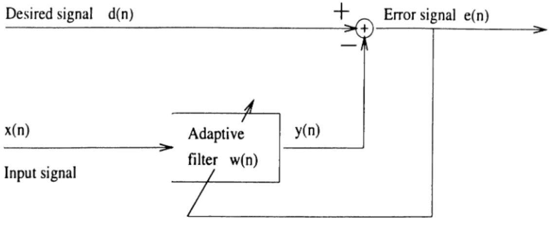
A typical adaptive filtering configuration is shown in Fig. (2.1). The conven tional LMS algorithm has the following simple update:
w{n + 1) = l£(n) -f i.ie{n)x{n) , (
2
.1
)where /i is an adaptation constant, w{n) is the column vector of the tap weights of the adaptive filter at time n and x{n) is the column vector of the N most recent samples of the input at time n. i.e.
w { n ) = [lUi(n) lU2(?i) · · · Wn(^·)]^
x{n) = [;r(?i) x{n — 1) . . . x{n — A^ -t- 1 )]^
(2.2)
(2.3)
Figure 2.1: Adaptive filtering block diagram
The output error at time n is given by
e(n) = d{n) — iv^{n)x{n) . (2.4)
Equation (2.1) simply says that the coefficients of the adaptive filter at each iteration equal to the coefficients of the filter at previous iteration plus a term proportional to the product of the error and the data vector. It requires a total of 2N multiplications and 2N additions to update filter coefficients at each iteration.
In spite of the appearant simplicity of the LMS algorithm, analysis of the behavior of the filter is difficult. Although a considerable amount of work has been done, the results have been obtained for certain limited types of signals. Following results are obtained for white inputs assuming the independence of x{n) and w{n).
2.2.1
Convergence In the Mean
It has been shown that [2-7] for stationary inputs the LMS algorithm converges to the following optimal Wiener solution provided that it is stable
lim £^M n)] = lii = Rrxtxd (2.5)
where = E{x{n)x^{n)] and = £ '[¿(
77
)1
(71
)]. The stability is guaranteed if the adaptation constant p satisfies the following condition•7
wliere Am„j. is the maximum eigenvalue of the input auto-correlation matrix /¿xr· By defining parameter error vector as
v{n) = -£[i£(n)] — ui it w'as found that the filter coefficients evolve as
u,(n + 1) = (1 - /zA,)u,(n); .
(2.7)
(
2
.
8
)
¿From this equation the time constant for the convergence of the mode is estimated to be
ti 1
f l \ , (2.9)
The overall speed of the convergence is clearly limited by the slowest converging mode which in turn stems from the smallest eigenvalue;
1
(
2.
10)
By substituting the upper bound found for the adaptation constant we get
t
AmiTi (
2
.11
)This means that the rate of convergence of the LMS algorithm is governed by the eigenvalue spread or the condition number of the input autocorrelation matrix [7].
2.2.2
Convergence In the Mean Square
Although the LMS algorithm converges to the optimal Wiener solution in the steady-state, noise in the adaptation process causes the steady state solution to vary randomly about the minimum point. This results in a steady-state mean square error J{n) which is greater than the minimum mean square error Jmin- The steady-state mean square error can be expressed in terms of the tap weight error vector as
J{n) = Jmin + {m{n) - w’ f {m{n) - w’ ) — Jmin T 11 (^^).^rrll(^0
(2.12)
(2.13)
We (k'iine the excess mean scpiare error as the difFerence between the mean .s(iuare error, produced by the adaptive filter at time n and the minimum value that can be achieved which is given by
J t x — Jmin ■ (2.14)
The ratio of the excess MSE to the minimum MSE is defined as the misadjust- ment [2]. It has been shown that for small values of fi the misadjustment is given by
M = . (2.15)
For la-rger values of //, Nehorai and Malah provided the following result [31].
« - r f S c
It is seen that for ptrRxj. <C 1, the misadjustment linearly varies with fi, which is an intuitively evident result.
2,3
The Nonlinear LMS Algorithm (N LM S)
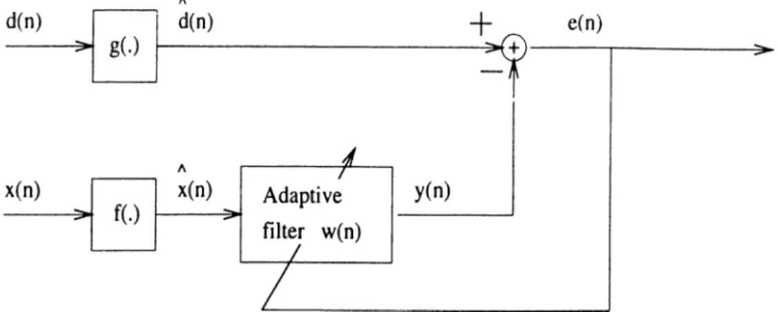
The proposed algorithm is schematically represented in Fig. 2.2, and it has the following weight update equation:
w{n + 1) = w{n) + fie{n)x{n) where
e(n) =
d{n) —¿(n)^u?(n)
,and
x{n)and
d{n)are given by:
i ( " ) = I / ( ' f ( ' · ) ) - - ^ + l ) ) t d(n) =
(2.17)
(2.18)
(2.19) where / and g are memoryless odd-symmetric nonlinear functions.
As it is evident from the structure of the proposed adaptive configuration, NLMS algorithm is based on the conventional LMS algorithm but incorporates nonlinear transformations of the input and the desired signals. The primary function of the nonlinearity is to decrease the eigenvalue spread of the input aul.ocorrela.tion matrix. Later, we will show how to use a proper nonliiu'arity
Figure 2.2; NLMS block diagram
to filter a-stable non-Gaussian processes, and processes which are corrupted by additive impulsive interference.
In this chapter we consider only the case in which f = g. We found the following so-called softlimiter nonlinearity most useful in our studies:
f{^ ) = <
a if X > a
X if — a < X < a —a if X < —a
Analysis of the effects of the softlimiting on the correlation function of the input data is difficult, and analytical results are hard to obtain. We have explic itly evaluated the autocorrelation function of a softlimited correlated Gaussian process by approximating the softlimiter with a continuous differentiable func tion. According to the results presented in Section 2.4, softlimiting a correlated Gaussian process causes a decrease in the autocorrelation coefficients:
p{m) < p{m) ■, 777 = 1 ,2 ,...
(
2
.
20
)
Hence, the softlimiting can be viewed as some kind of a decorrelation opera tion which flattens the spectrum of the input process. Since the ratio of the maximum eigenvalue to the minimum eigenvalue is bounded by the ratio of the largest to the smallest component in the power spectrum [2], the previous statement implies that the condition number of Rj-r can actually be decreased by such a transformation. While this explanation may not be valid for all types of input data and cannot be taken as a proof, simulations have shown t hat t hisis the case for all but a few exceptional cases. The following examples are presented to confirm the credibility of the conclusions drawn in this section. E xa m p le 1. Consider a first-order auto regressive process (.\R(1)):
x{n) = ax{n — 1) -f u{n)
(
2
.
21
)
where u(n) is a random zero mean i.i.d. Gaussian process with variance a^. It is well known that the normalized autocorrelation function of this process is:p{m) = o'" . Therefore R^x at order N takes the following form
(
2.
22)
R'XX --1 a,N-1
a1
,N-2 a a , N - 1 ,A f -2 (2.23)The eigenvalue spread of Rxx, x{Rxx) —_ A increases as a —> 1 and it is a monotonie nondecreasing function of the order of the matrix N. The case for which a = 0 corresponds to the input being white , x{Rxx) = 1, and we obtain the highest possible convergence rate for LMS adaptation.
Let us take 2000 samples of an AR(1) process with a = 0.99 and cr^ = 1 — 0.99^. The process was passed through a softlimiter and the variation of the condition number is plotted in Fig. 2.3.a as a function of the clipping value of the softlimiter as it varies from 3ctj. to O.OIcti. For a = 3, x{Rxx) = 626 and for a = 1, x (/?
3
;x) = 456. Using NLMS with a = 1 instead of pure LMS in this case would speed up the convergence of the filter coefficients by a factor of roughly equal to 1.37.E x a m p le 2: Consider a signal x{n) which is obtained by passing a zero mean white Gaussian process through a 32"*^ order linear phase FIR noise coloring filter. The frequency response of the coloring filter is given in Fig. 3.3.a. x{n) models a correlated Gaussian process whose autocorrelation sequence is the autocorrelation of the filter impulse response since the input to the coloring filter is white. Eigenvalue spread of Rxx at order = 7 is x{Rxx) = 2096.
Again, 2000 samples of x{n) passed tlirough a softlimiter with varying clip ping value were used to estimate the condition number of the process at order 7.
Figure 2.3: Variation o f condition number as a function of clipping value of the softlimiter. Upper curve corresponds to the AR(1 ) process, and the lower curve corresponds to the colored noise.
The variation of the condition number is plotted as a function of alpha in Fig. 2.3.b . The plot shows that the condition number decreases with decreasing clipping, which confirms our intuitive explanation.
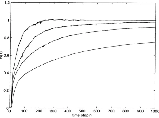
The produced signal x{n) was used to perform a system identification exper iment, where the desired signal was derived by passing the input through a order FIR filter A = [1 0 . . . 0]^, which is the model system. At convergence coefficients of the adaptive filter may be taken to be the estimates of those of the model system, hence the name system identification. Both the LMS and the NLMS algorithms were used in the adaptation and the convergence o f the first tap weight of the adaptive filter is plotted in Fig. 2.4, by averaging the results of 100 simulations. The upper curve corresponds to the lowest value of the clipping and the clipping value decrease as we move down the curves. The slowest converging curve belongs to LMS. The stepsizes of LMS and NLMS
were adjusted to have the maximum possible rate of convergence without en countering the danger of instability. As observed, it is possible to obtain much higher convergence rates using the NLMS algorithm in the adaptation.
Figure 2.4; Convergence curve of the first tap weight for different degrees of clipping.
2.4
Convergence Analysis
So far we have only dealt with the implications of softlimiting on the eigen value spread of the input autocorrelation matrix, and we have seen that such a transformation could be used to decrease x{Rxx). On the other hand, ap plying a softlimiting operation to the input and the desired signals certainly changes the underlying statistics of these signals. Therefore we cannot expect the NLMS algorithm to converge to the same solution provided by the LMS.
In this section we will try to derive expressions for the mean weight provided by the NLMS algorithm at convergence. The analysis is based on computing
the desired statistics of the softlirnited processes by approximating the softlim- iter with a continuous differentiable function.
In order to simplify the analysis, we will use the following analytic function to approximate the soft nonlinearity
/ ( - ) = V 7Г (J Jo
f
dz (2.24) Here, the scalar parameter a controls the sharpness of the nonlinear func tion at the origin and the degree of saturation. The behavior of f { x ) can be varied by changing a. For exampleand l i m /( x ) = sign[x] lim f { x ) = \ - — cT-fOo у 7Г a (2.25) (2.26) Therefore the hard limiter and the linear function are limiting cases of (2.24). We assume that the input signal is a stationary Gaussian process with zero mean and variance al. i.e.
E[x{n - i)x{n - ;■)] = fiij гф j . (2.27) We will assume that the following relationship exists between the input and the desired signals:
d{n) = x{n) (2.28)
Inserting this into the NLMS update we get
w{n + 1) = w{n) +
/1
[/(A ^ x (n )) - m ^ (n )/(x (n ))] f { x { n) ) (2.29) In this case, the parameter error vector isv{n) = w{n) — h (2.30)
By writing the NLMS update in terms of the parameter error, vector we get v{n + 1) = £(7J.) + f i f { hj x{ n) ) f { x{ n) ) - fi f { x{ n) ) f { x^{ n) ) v
Taking the expectation of (2.31) and assuming that the parameter error vector and the data vector x{n) are independent of each other we obtain
E[v{n +1)1 = E[v{n)] + nE[ f i l Jx{ n) } f { x{ n) ) ] (2.32) -fiE[f{x{n)}f{^^{n))]E[v{n)] - fiE[f{x{n))f{x^(n))]E[h] Thus the right hand side (RHS) of (2.32) requires the evaluation of the non linear Gaussian functionals of the form
and
E[ f { ! /x { n) ) f { x { n - i))];
2
= 0 , - 1 (2..33)E [ f { x { n - i ) ) f { x ' ^ { n - j))]] = 0 , 1 , . . . , 7 V - 1 . (2..34) The desired expectation involves nonlinear functionals of a pair Gaussian vari ates which can be evaluated by using Price’s theorem, which is stated in the following paragraph:
P r ic e ’ s T h e o r e m : Given two jointly normal RVs x and y, we form the mean / 00 roo
/ g { x , y ) f { x , y ) dx dy . (2.35)
-oo J — oo
of some function g{x, y) of {x,y). The above integral is a function 1(g) of the covariance g of the RVs x and y. Then
d^I{g) d^^g{x,y)
t"
J-oo J-
J-oo J-OO dx'^dy'^
f { x , y ) dx dy = E dx^dy'^ (2.36) The advantage of this approach is that it is often not possible to directly evaluate ^[^'(a;,y)]. However, the expectations of the derivatives of g{.) can usually be evaluated easily so that, the desired expectation can be formed by integrating over g.By using this theorem, we first evaluate E[ f { x{ n — i ) ) f { x{ n — j) ) ] . Let X{ = x{n — i) and Xj — x{n — j). x, and Xj are jointly normal with zero mean and covariance E[xiXj] = /i,j. Appljdng Price’s theorem to the unknown expectation d l j g ) d g = E d f { x i ) d f { x j ) dX, d X j (2.37) 7T a
2
1
2 1
7T
J-IX, J-co 2n
1M
|l/2 f ia’i (■'2=-where x = [x,
M "' =
-1
/' 1
(2.38)
and I M 1= det{M) = a\ — fp. The integral in (2.37) can be put into the following form dlifi) 2 I \ K 1 dn 7r(r2|M|i/2 oo 27T I K p /2 where
K-^ =
-Zl— 4. X JZJL. JZJL. +^
(2.39) (2.40) and K 1= det{K) = 1 ^2 + 2 ^ · 1 ^ cr'i I 1 det{K ^) — ¡x^ ' cr^+ - 7 (2.41) The integral in (2.42) is equal to one. Therefore we have the following resultdl { n) 2 1 I A' 2 1 1 1
dyi
» V <7^ <7^ <2.42)1
7T
\/r)'^ —
where t]'^ = a* + 2alcr^ + a*. By integrating the above expression with respect to y and putting the initial condition 7(0) = 0, we arrive at the following expression
A " ) = ? 'i” · '
[ f ) = l
=“ ■' ( ? r ^ ) (2 ·« )Next, we need to evaluate E[ f { f Xx{ n) ) f { x{ n — ?'))]. The desired response d{n) = iXx{n) and the components of x{n) are jointly distributed Gaussian variates with zero means and with variances and covariances given by
/i, = E{h^ x{n)x{n — ?')] = 4 ^r(i) (2.44)
A[d^(n)] = iX E[x^{n)x{n)]h (2.45)
= ¡X RtxIl (2.46)
wliere
r ( i ) = [7’ (?) ?'(?' + 1 ) . . . r(?’ + .'V — ] )]
r{i) = /¿'[.7:(77).'r(77 — ?)]
( 2 .4 8 ) ( 2 . 4 9 )
Thus we see that the form of the expectation is the same as the one in (2.34). By carrying out the same steps from (2.37) to (2.43) we obtain the following result
E[ f { h^x{ n) ) f { x{ n - i))] = - sin- 1 (2.50)
7T \cr2 + <Jxb^ R x x k J
Therefore the input autocorrelation matrix and the vector of crosscorrelations between the input and the desired signals are given by
R'XX -- sm- 1 7T
2
Ixd = i - sin 7T - 1 ' E[x{n — i)x{n — j ) ' h^r_{i) \ 1 •j (2.51) (2.52) T ^ x k . R 'x x k j J j'Substituting (2.51) and (2.52) in to (2.32) yields
u
(
t7 + 1) =: (/ -
fiRrx)v(n)+ /i(r^rf -
Rxxk)(2.53)
Hence, we find that the parameter error vector v{n) converges in the mean to
E[v{n
+ !)]->
- k (2.54)provided that the algorithm is stable. It is assumed that the modified input autocorrelation matrix Rrx is invertible.
The expression found for the bias of the parameter error vector at conver gence is not sufficient for describing the convergence properties of the NLMS algorithm. It is necessary to describe the time evolution of the parameter error vector and find an expression for the stability range of the algorithm in terms of the adaptation constant. In order to do this, we define a new parameter error vector as
v{n)
=
£^[u(n)]- R;^tc¿ +
k.
(2.55) We can rewrite (2.31) in terms of v{n) asWe now have a recursive equation which describes the evolution of tlie error in NLMS coefficients. First, we try to decouple the update equations by di agonalizing positive definite symmetric matrix Rj:^. R^^j. can be decomposed as
Rxx = Q^AQ (2.57)
where Q is the modal matrix which has normalized eigenvectors of R^^ as its columns
<3 = lii
£2
■ · ■ i « l ·Q'^Q = I
(2.58) (2.59) where q. is the eigenvector corresponding to A,. A, the so called spectral matrix, is a diagonal matrix whose diagonal elements consist of the eigenvalues of R^^
A = Ai 0 0 A
2
0 0 0 0 0 Xn (2.60)Returning to equat^ion (2.56) and substituting (2.57) we get:
v { n 1) = {I -
hQ'^AQ)v{n)
(
2
-
61
)
The matrix Q is now used to defined the rotated error vector u{n + 1)
u(n) = Qv(n) . (2.62)
Multiplying both sides of equation by Q and using the fact that = / we arrive at the following equation
u(ji + !) = ( / — /iA)u(n + 1) (2.63)
In view of the diagonal nature of A, we can separate decoupled equations for each element of u(n) as
This first-order scalar difference equation can be solved by using repeated sub stitution, providing the following result
u . ( n + ! ) = ( ! - A ) ”m.(0) . (2.65) Therefore, in the limit
lim u:(n + 1) = 0 n —oo ^ (2.66) provided that 2 0 < n < — A.· (2.67)
Hence, the condition for convergence is
^ 2
0 < f i < . '^max
(2.68)
where Xmax is the largest eigenvalue of Rxx. On the other hand, the time constant for the convergence of T** mode can easily be calculated as
u 1
f i X i
(2.69)
The convergence rate of the NLMS algorithm is clearly limited by the mode which has the smallest eigenvalue Combining equations (2.68) and (2.69) we have the following expression for the time constant of NLMS algorithm:
t \ X. ~ A Amin (2.70)
Therefore we see that the NLMS algorithm converges in a time proportional to the eigenvalue spread of the autocorrelation matrix of the softlimited input data. In section 2.3, we intuitively argued that passing input through a soft- limiter decreases the eigenvalue spread. Therefore, based on this argument, we can say that Inlms <
The above analysis has been carried out for / ( . ) = g{.) and in particular for / being a softlirniter. Under these restrictions it is seen that the algorithm is biased. An interesting question is whether we can remove the bias entirely by using a different structure for the AF configuration. If d{n) = f { x { n) ) , the RHS of (2.57) becomes
and NLMS is an asymptotically unbiased estimator. Furthermore the evolution of the parameter error vector is governed by the properties of the modified input autocorrelation matrix R^x. Thus, NLMS converges m uch fa ster to the optimal Wiener solution if a suitable structure can be found to have d{n) — f { x{ n) ) . This kind of an exact relation betvi'een the input and the desired signals can be obtained in system identification applications where the input to the plant is nonwhite[A2\. The modified NLMS structure is schematically represented in Fig. 2.5.
2.5
Computer Simulation
Let x{k) = aix(A:—l)-fa23'(^—2) +u(7?) be an AR{2) process, where a\ = 1.9114 and
02
= —0.95 and {o(A·)} is an i.i.d. white noise sequence. The input signal to the adaptive filter was x\n)^ and the desired signal was d[n) = x{n + 1). In Fig.2.6 transient behavior of the tap weights provided by the LMS and NLMS adaptation algorithms are plotted. The step size fiiMS = 0.11 was adjusted so that the LMS adaptation was at the edge of instability. The step size of the NLMS adaptation was /x/vlms = 0.4 and the input and the desired signals were clipped at a = The plot shows improved convergence rate of the NLMS relative to the LMS. The final values of the tap weights of the NLMS and the LMS are different due to the bias introduced by the nonlinear transformation of the input signals.Figure 2.6: Transient behavior of tap weights. Solid line dashed line
yiLMS-2.6
Steady State Mean Square Error
In the previous section, we derived expressions for the mean weight at conver gence of the NLMS algorithm, and obtained bounds for the stability range o f ' the algorithm. However, the analysis of the convergence behavior in the mean is of limited value without obtaining results for the behavior of the system about the steady-state solution. In this section, we will be concerned with the analysis of the mean square error J{n) and misadjustment for the adaptive filter.
As described in section (2.2.2), the mean square error can be written as = «^min + ^ {ri)Rxj:v{n) (2.72) where ii{n) = w{n) — R~lfxd., is the parameter error vector as defined in section (2.4). Using (2.57) and (2.62), (2.71) can be put into the following form
J{n) = Jmin + M^(n)Au(n) (2.73) where u{n) = Qv{n) and Rrr = Q^AQ. The elements of the diagonal of A are the eigenvalues of the autocorrelation matrix. Equation (2.71) can be rewritten
as
N
J{ti) — Jmin ^ ^ (2.74)
k=\
where u^.(n) is the k*^ element of the vector Taking the expectation of both sides
N
£ [J (n )] = ^ A i£ [«i(n )) (2.75)
k=l
From now on we will assume that the convergence of the algorithm has taken place in the steady state. Steady-state value of J{n) will be denoted as Joo· The NLMS algorithm uses an estimate of the gradient at each iteration [l]-[2]. The update equation can be written as
w{n + 1) = m{n) - fi^{n)
where V is the estimate o f the gradient. It can be written as
V ( n ) = V ( « ) + £(«)
(2.76)
(2.77) where V ( ” ) is i'h® gradient and e{n) is the noise of the estimate. Sub stituting (2.77) into LMS update and using v(^^) = 2Rxxw{n) — 2rxi [7] we have
v{n + 1) = 2 ( / - fiRxx^ v{n) — fi£{n) (2.78) Multiplying both sides of (2.78) by Q
u{n + 1) = 2 ^7 — m(»^) “ (2.79) Assuming wide-sense stationarity at convergence and taking the covariance of both sides
4(A — //A^)cov[u(n)] = /rcov[e(7j)] (2.80) Since at convergence the exact gradient is zero
[£(»)] = -2e{n)x{n) . (2.81)
At convergence the error is orthogonal to the input vector. Thus, we get
cov[t(n)] = (5^cov[e(7?.)]Q (2.82)
= 4Q^RxxQE[c\u)] (2.83)
Since, E[t^{n)] converges to the steady-state MSE
cov [ e( n) ] = 4 A .
By substituting (2.85) into (2.82) we obtain
E [ ^i {n )] = {cov[ u( n) ] } , . _,
~ /r«/o 1 1 - ^i\i, Now, by using (2.75) we obtain
^ / 1 ■
J (x j
— lim EJ[t/(n)j — <7inin “h ^ ^
ooI
For this case, the misadjustment is
j o o "Anin
M = - ^ *Anin
By using (2.89), the corresponding misadjustment is found as 7T M = 1 - 7t’ ¿ t U - A . N By using y~^ /r A, = fxtrRi t = l
we find that the misadjustment is given by
M = fitrRx
(2.85)
(
2.
8 6)
(2.87)(
2.
8 8)
(2.89) 1 — fitrRx (2.90) (2.91) (2.92) (2.93) (2.94)2.7
Performance of N LM S Under Additive
Impulsive Interference
It lias been known that the LMS algorithm may degrade unacceptably when the input signals are corrupted by impulsive interference [7]. Sparse impulses
arise in a. variety of practical applications such as speech, biomedical and image processing. The proposed algorithm suggests an improvement in the perfor mance over the LMS in such situations.
The new configuration can be useful in applications where additive impul sive interference is a problem. The nonlinear transformation of the input sig nals protects the filter coefficients from the impact of impulsive interferences b}' limiting the magnitude of the sparse impulses. Unlike other LMS variants de veloped to cope with the impulsive interference problem, the proposed method does not introduce additional computational effort.
Consider an adaptive filtering configuration where the input and the desired signals are corrupted by impulsive interferences ^(??) and r]{n) respectively.
x'{n) = x{n) + ^{n) d'{n) = d{n) -f 7/(n)
(2.95) (2.96) Here we assume that the impulsive interferences ^(n) and T]{n) are zero mean i.i.d. sequences which are mutually independent and are independent of both x(n) and d{n). We also assume that the input sequence is i.i.d. with <7^ = 1. We assume that the following relation exists between the desired signal and the input signal:
d{n) = h}x{n) . (2.97)
We will examine three different cases 1. ^(n) = 0 7/(n) = 0 for all n. 2. ^(n) = 0 for all n.
3. 7/(n) = 0 for all n.
Throughout the analysis the impulsive signals will be assumed to have the following form
C(n) = c(n)y4(n) (2.98)
where c(n) is an i.i.d. sequence with
P{c{n) = 1] = a; P {c (n ) = 0} = 1 - a (2.99) where a is the arrival probability. The distribution of the amplitude /l(n ) is arbitrary subject to the constraint that var{A{n)} > cr^. Wo will assume that the amplitude is independent of the arrival time.
C ase I. In this case the relation between tlie injnit and the desired signals is exact and LMS algorithm converges to the following optimal set of coefficients provided that the algorithm is stable[2]
Lxd
(
2.
100)
where Rxx = E[x x‘ ] and = E[xd\. C ase II. In this case input signals are
and
d'{n) — d{n) + T]{n)
x'(n) = x(n)
(2.101)
(
2.
102)
Defining the parameter error vector as v(n) = w(n) — A, the LMS update can be written as
v(n + !) = ( / — /^x(n)x\n))v(n) + //x(n)?/(n) . (2.103) Taking the expectations and assuming that the input signal x(n) is independent of the parameter error vector v(n), we get
E[v(n + 1)] = ( / — /J'E[x{n)^{n)])E[v{n)] . (2.104)
With x(n) an i.i.d. sequence as assumed, E[x{n)x^{n)] = and the parameter estimates are in the mean decoupled. This means
£?[u,(ii + 1)] = (1 - ^cr^)£'[u,(/?.)] I = 1 , 2 , ...,7V (2.105)
If we choose 0 < fi < 2/crl the algorithm converges to
l£co = = ¡1 · (2.106)
Hence, in this case the parameter estimates are unbiased as in Case I. However, their variances are not smaller than those in Case I.
C ase III. In this case we have
and
d'{n) = d{n)
.r'(n) = x(n) + ({n)
(2.107)
The parameter error equation becomes
£ (n + l) =
2
z(n)+/i [x\n)h - ix(n) + ^{n)yv{n) - {x{7i) + ^ (n ))‘A] (T(?7)+i(7?)) (2.109) Taking expectations we obtainE[v{n + 1)] = / - n{E[x{n)x^{n)] + .^[¿(i7)^'(n.))].E[i;(n)] - /x.E[£(n)^'(n)]A (2.110) The above equation decouples to give for the component of the parameter error vector
E[vi{n +
1
)] =[1
- fi{crl + cr|)]£;[t;,(7
i)] - ficr^hi Thus LMS algorithm converges to(2.111)
UL·^ = (2. 112)
Therefore in this case the LMS does not converge to the optimal parameter set and the bias is given by
E[v{n + 1)] (2.113)
We see from (2.115) that the bias is proportional to the variance of additive impulsive noise. If we use a softlimiter which produces negligible distortion on the input and the desired signals but greatly decreases the variance of the impulsive noise component we can get a smaller bias. In other words, we want
f{ x {n ) + ^{n)) Ä! x{n) + f { ( {n ) ), g{d{n) + i]{n)) « d { n ) g { i ] { n ) )
(2.114) (2.115) where / ( . ) and g{.) are softlimiters whose clipping values are adjusted to yield minimal distortion on the input. Carrying out the analysis for the three cases considered above we obtain the following results:
Case I.
The relation between the input and the desired signals are not aifectedand NLMS converges to the optimal set of coefficients as in (2.108).
Case II.
Replacing d{n)-\-r}{n) by d{n) + g{7]{n)) we see that NLMS convergesC ase III. Replacing
1
(77
.)+ (^(n.) by /(3-(77)+ ^(77
)) = x(7?.) + /(^ (n )) and retrac ing the analysis in (2.107) through (2.113), we obtain the following expression for the bias in the mean parameter error vectorA 2 F;[u(77-f 1)]
-7
2
^2
^tI + crl (2.116)
»1 = B | /"(i(n ))]. (2.117) where
A convenient way is to set the clipping value of the softlimiter to three stan dard deviations above the mean of the input signals (assuming the signals are Gaussian distributed), since the effect of softlimiter on the correlation function of the input is practically absent for this value.
2.7.1
Computer Simulation
The potential of NLMS algorithm is illustrated in a simple adaptive filtering problem by considering the effects of impulsive interference. Let a;(77.) = d{n) where x{n) is an i.i.d. Gaussian input with a"l — 0.01. The impulsive interfer ence has the form
7
/(77
) = c„A „ (2.118)where c„ is i.i.d. with
p(c„ = 1) = 0.02; p(c„ = 0) = 0.98 (2.119) The distribution of the amplitude is Gaussian with var{A/t) = 1 and mean zero. The impulsive noise is added to the input signal x{k). The transient behavior of tap weights for the NLMS and the LMS is plotted in Fig. 2.7 by averaging 50 independent trials. The parameters chosen for this simulation were: filter length N = 2 , step size
/7
= 0.2 and the clipping point of the soft-limiter a = 0.2. The LMS performed poorly in the presence of impulsive interference and failed to converge to the optimal solution w* = 1. In contrast the NLMS algorithm exhibited a smooth convergence and a much smaller bias.Figure 2.7: Convergence curves of NLMS(dotted) and LMS(solid) under addi tive impulsive interference
2.8
Adaptive Filtering Approaches for Non-
Gaussian Stable Processes
Another application of our method is adaptive filtering for non-Gaussian sta ble processes [40]. There is a large class of physical phenomena which exhibits non-gaussian behavior such as underwater acoustic noise, low frequency atmo spheric noise and many types of man-made noise. They exhibit sharp spikes and occasional bursts in their realizations. In the modeling of these type of sig nals and noise o-stable distributions can be used. Formally, a random variable is called a-stable if its characteristic function has the following form:
where —oo < a < o o ,
7
>0
, 0 < a < 2 , andw (/.,a) = < tan(Q7r/2) for q; 1 f log|i| for a = 1
(2.121)
There is no explicit expression for the probability density function of these random variables except for or = 1 and 2, which correspond to the Cauchy and Gaussian distributions, respectively. The characteristic exponent q is a measure of the deviation of the distribution from Gaussian. As a approaches zero the tails of the distribution function becomes heavier. For 1 < a < 2 the a-stable processes fail to have second or higher-order moments. As a result, many of the adaptive filtering algorithms which are based on the minimization of mean-square cost function become useless.
There are a number of solutions suggested to solve the minimization prob lem mentioned above with the motivation of gradient decent algorithms [28]- [40]. Such an algorithm, least mean p-norm (LMP) algorithm, is proposed in [40]. This algorithm is a generalization of instantaneous gradient descent algorithm to a-stable processes, where the gradient of the p-norm of the error.
J = fi(|e(n)|']
= E[\d{n) — w{n)'x{n)\^], 0 < p < a
(
2.
122)
is used, and the tap weights, w, are adapted at time step n + 1 as follows: w{n + 1) = m.{n) -h p [e(n)|'’“ ^sign[e(n)] x(n) (2.123) where p is the step size which should be appropriately chosen. Note that, for p = a = 2 the LMP algorithm reduces to the well-known LMS algorithm [1]. When p is chosen as 1, the LMP algorithm is called the Least Mean Absolute Deviation (LM AD) algorithm [40]:
w{n + 1) = iv{n) + /isign[e(?i)] x(n ) (2.124) which is also known as the signed-LMS algorithm. With the motivation of the Normalized LMS algorithm. Normalized Least Mean p-Norm (NLMP) algo rithm and Normalized Least Mean Absolute Deviation (NLM AD) algorithm were introduced in [28], with a superior performance than those of LMP and LMAD.
The normalized Least Mean p-Norm (NLMP) algorithm, uses the following update:
w{n + 1) = w{n) + /3 e(n)|P h\gn{t(n))
\l + x x { n ) (2.125) where /3, \ > 0 are appropriately chosen update parameters. In (2.125) nor malization is obtained by dividing the update term by the p-norm of the input vector, x{k). The regularization parameter. A, is used to avoid excessively large updates in case of an occasionally small inputs. For p = 2, NLMP reduces to the Normalized-LMS algorithm [1].
The second algorithm. Normalized Least Mean Absolute Deviation (NL- M AD), corresponds to the case of p = 1 in (2.125) with the following time update:
crnipi ri/\l
(2.126) w{n + 1) = w{n) + /?
|ai(n)||i + A
This adaptation scheme is especially useful when the characteristic exponent, a, either is unknown or varying in time. Among the stable distributions the heaviest tail occur for the Cauchy distribution, a = 1. By selecting p = 1 the update term is guaranteed to have a finite magnitude for all 1 < a < 2. Because of these reasons the NLMAD is a safe choice for the adaptation.
2.8.1
Use of Pre-nonlinearity in Adaptive Filtering
In this section the performeince of the LMS and the RLS algorithms running on nonlinearly transformed data will be investigated. In this section, we consider the use of a softlimiter. The motivation behind this approach is to be able to reduce the effect of spiky characteristic of the a-stable data.This type of regu larization have been used in robust signal processing applications [41]. It can be easily shown that any random process which is passed through a softlimiter has finite variance. Thus, the LMS and the RLS algorithms can be used in adaptation process after the input and reference signals have been soft-limited. The optimal filter coefficients which LMS and the RLS converge are biased. However, the bias so introduced can be kept at a reasonably small level by a. proper selection of the threshold value in the softlimiter. The use of softlimiter reduces the spiky characteristics of input data hence a much smoother conver gence can be expected. One noteworthy feature of this technique is t hat it has the same computational complexity as well-known LMS and RLS algorithms.
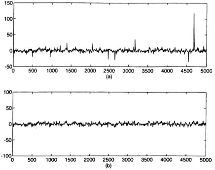
Because of the nonlinear mapping involved we call the proposed algorithms as the NMLMS and the NMRLS. A sample sequence of A R process disturbed by Q'-stable ( o = 1.8) noise and the output sequence after the softlimiter are shown in Figure 2.8. 0 500 1000 1500 2000 2500 3000 3500 4000 4500 5000 (a) 100 -100 0 500 1000 1500 2000 2500 3000 3500 4000 4500 5000 (b)
Figure 2.8: A sample A R process disturbed by a-stable (a = 1.8) noise (a), and the output process after the soft limiter (b).
2.8.2
Computer Simulations
In simulation studies we consider AR{N) a-stable processes, which are defined as follows,
N
x{n) = ^2aix{n — i) + u{n) (2.127)
t = l
where u{n) is a a-stable sequence of i.i.d random variables. The common distribution of u{n) is chosen to be an even function {/3 = 0), and the gain factors are all set to one (
7
=1
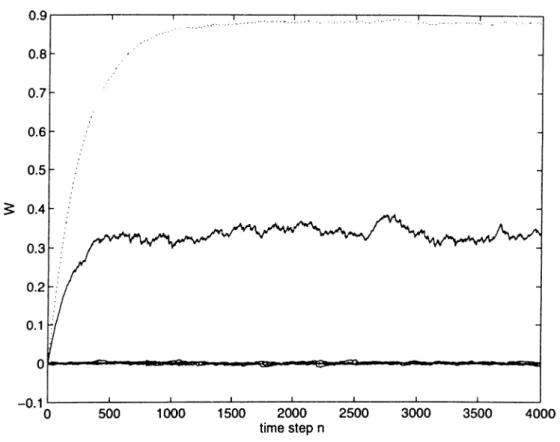
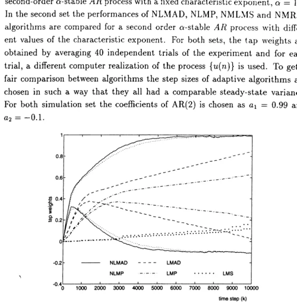
) without loss of generality. It can be shown that a;(n) will also be a a-stable random variable with the same characteristic exponent when {a.,} is an absolutely summable sequence [40].Two sets of simulation studies are performed. In the first set, the adapta tion algorithms NLMAD, NLMP, LMAD, LMP and LMS are compared for a.
second-order a-stable AR process with a fixed characteristic exponent, q = ] .2. In the second set the performances of NLMAD, NLMP, NMLMS and NMRLS algorithms are compared for a second order a-stable AR process with differ ent values of the characteristic exponent. For both sets, the tap weights are obtained by averaging 40 independent trials of the experiment and for each trial, a different computer realization of the process { « ( n ) } is used. To get a fair comparison between algorithms the step sizes of adaptive algorithms are chosen in such a way that they all had a comparable steady-state variance. For both simulation set the coefficients of AR(2) is chosen as ci = 0.99 and 0,2 = —0.1.
Figure 2.9: Transient behavior of tap weights in the NLMAD, NLMP, LMAD, LMP and LMS algorithms with a = 1.2.
In the first part of the simulations, AR parameters a are estimated by a 2”*^ order LMP, LMAD, NLMP, NLMAD and LMS algorithms. The plot of the tap weights is given in Figure 2.9. In the first part we observed that the normalized algorithms NLMAD and NLMP outperformed other algorithms. Therefore, in the second part the performances of NMLMS and NMRLS are only compared to NLMAD and NLMP algorithms.
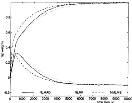
In the second part of the simulations, AR parameters a are estimated by a 2"*^ order NLMP, NLMAD, NMLMS and NMRLS algorithms for two different a-stable AR processes with a = 1.2 and a = 1.8. The plots of the tap weights
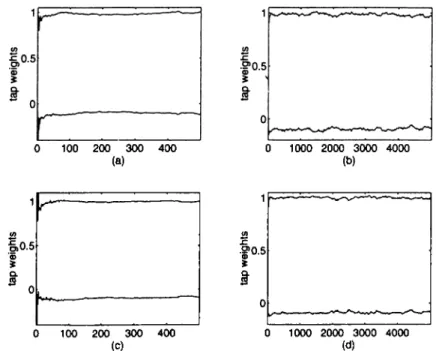
for NLMAD, NLMP and NMLMS algorithms are given in Figure 2.10 and Figure 2.11 for O' = 1.2 and a = 1.8, respectively. The convergence performance of the tap weights for the NMRLS is given in Figure 2.12 for a = 1.2 and a = 1.8.
time step (k)
Figure 2.10: Transient behavior of tap weights in the NMLMS, NLMAD, NLMP algorithms with a = 1.2.
2.9
Conclusion
In this chapter we present a new adaptive filtering algorithm which utilizes nonlinear transformation of both the input and the desired signals. The new algorithm has a number of useful features such as improved convergence speed, the capacity of reducing the spiky characteristic of the input data and operating under additive o-stable noise. Its major drawback is a bias introduced by the nonlinear transformation.
time step (k)
Figure 2.11: Transient behavior of tap weights in the NMLMS, NLMAD, NLMP algorithms with a = 1.8. 0 100 200 300 400 (a) 0 1000 2000 3000 4000 (b) if) 1.0.5 'S
Q.
^ 0 0 100 200 300 400 (C) 1r
' '—' '' " r--- -■ ■ ■■ L , |0.5 t 0 0 1000 2000 3000 4000 (d)Figure 2.12: Transient behavior o f tap weights in the NMRLS algorithm with Q = 1.8 (a),(b), and a = 1.2 (c),(d).
Chapter 3
USE OF A PREWHITENING
FILTER IN LMS
ADAPTATION TO
INCREASE CONVERGENCE
SPEED
3.1
Introduction
The LMS algorithm is one of the most widely used algorithms for adaptive filtering due to its robustness and simplicity. Unfortunately, its convergence speed is highly dependent on the eigenvalue spread of the input autocorrelation matrix. There had been attempts in the past to improve the conditioning of the input correlation matrix by decomposing the input signal into a set of partially uncorrelated components via an orthogonal transform such as DFT or DCT. The main disadvantage of this type of preprocessing is the additional computational complexity introduced, and in the case of DFT, conversion of real data into imaginary data. It should also be noted that a fixed parameter
orthogonal transform may not give optimal results for all types of inputs signals. It is known that the RLS algorithm achieves near optimum convergence rate by forming an estimate of i?“ *, the inverse of the input autocorrelation matrix. This algorithm automatically adjusts the adaptive filter to whiten any input and also varies over time if the input is a nonstationary process.
In this chapter we present a new method to ameliorate convergence speed of the LMS adaptive filter. A linear filtering operation is performed on the input data and the desired signal to whiten the input signal while keeping the filter coefficients unaffected by the linear transformation. It is shown that the linear filtering of the input signal can decrease the condition number o f the input correlation matrix without introducing additional computational complexity if the filter order is chosen small. The coefficients of the linear filter is obtained from a small order adaptive filter which is expected to work very fast.
3.2
Proposed Adaptive Algorithm
The proposed adaptive configuration is schematically represented in Fig. 3.1 . Here, h = [1 — is an order whitening filter whose coefficients are obtained in a least-square sense by solving the following minimization problem
min J(Am-i) = S (^ (” ) “ - 1 ))‘ (3.1)
n = l
where i,^ (n — 1) is the data vector formed by M most recent samples at time
n — 1
— 1) = [®(n — 1) x{n — 2) . . . x{n — M + 1)]^ (3.2) Convolving the input and desired sequences by the filter h can be viewed as a linear prediction operation, where the current sample is predicted with a linear combination of M most recent samples of the input data. The error signal obtained as a result is fed to the adaptive filter which employs the LMS algorithm in the adaptation. Because of the linear filtering operation applied before adaptation, the proposed algorithm will be called as Linearly Filtered LMS (LFLMS).
Suppose that the relation between the input signal and the desired signal is given by d{n) = f^x{n). This means that the optimal Wiener solution for the tap weights converged by an A^th order adaptive filter is / itself. 'Fhe question
Figure 3.1: Adaptive filtering block diagram
here is whether the tap weights of the adaptive filter in the proposed system will converge to the same solution.
Suppose that the adaptation is performed by an A^-tap adaptive filter and the order of the linear filter h is M. After the transformation we define the following signals where d{n) = dj^f{n) x{n) = Xniin) d]^{n) = [d(n) d{n — 1) . . . d{n — M -\-\)Y (3.3) (3.4) (3.5) and XM{n) is as defined in (3.2). The relation between d{n) and i ( n ) can be found as follows d{n) = 4^dw(n) = A ^ K n ) d { n - l ) . . . d { n - M + \ ) f = A ^[/^£a/(^ ) - 1). .-fJxNin - M + 1)]^ M M
=
hmf^XN{n - m + 1) =
Y hruX^in
- 771+ 1) m = l m = l=
f l L ^ X M i n ) h^XMi n-
1) . . .
h^XMi n-
+
1)]^
= f x N { n )which is the same relation between x{n) and d{n). Therefore if the transformed input signal x{k) and the desired signal d{k) are fed to an adaptive filter, we expect that the adaptive algorithm converge to the same solution.