COMPARISON OF BAYESIAN AND STOCHASTIC MODELS
IN CLAIMS RESERVING WHEN THERE ARE NEGATIVE
VALUES IN THE RUNOFF TRIANGLE
Tevhide SERT
Supervisor: Yrd. Doç. Dr. Banu ÖZGÜREL
Department of Actuarial Science
Bornova-İZMİR
(MSc)
COMPARISON OF BAYESIAN AND STOCHASTIC
MODELS IN CLAIMS RESERVING WHEN THERE ARE
NEGATIVE VALUES IN THE RUNOFF TRIANGLE
Tevhide SERT
Supervisor: Assist. Prof. Dr. Banu ÖZGÜREL
Department of Actuarial Science
Bornova-İZMİR 2013
This study titled “Comparison Of Bayesian And Stochastic Models In Claims Reserving When There Are Negative Values In The Runoff Triangle” and presented as Master Thesis by Tevhide Sert has been evaluated in compliance with the relevant provisions of Y.U Graduate Education and Training Regulation and Y.U Institute of Science Education and Training Direction and jury members written below have decided for the defence of this thesis and it has been declared by consensus / majority of votes that the candidate has succeeded in thesis defence examination dated June 10, 2013.
Jury Members: Signature:
Yrd. Doç. Dr. Banu ÖZGÜREL ………...
Yrd. Doç. Dr. Serkan ALBAYRAK ………
ÖZET
VERİ ÜÇGENİNDE NEGATİF DEĞERLER BULUNDUĞUNDA
BAYES VE STOKASTİK MODELLERLE HASAR
REZERVLERİNİN KARŞILAŞTIRILMASI
SERT, Tevhide
Yüksek Lisans Tezi, Aktüerya Bilimleri Bölümü Tez Danışmanı: Assist. Prof. Dr. Banu ÖZGÜREL
Haziran 2013
Gelecek yıllar boyunca kademeli yapılacak olan hasar ödemelerinin negatif değerler alması, sigorta şirketlerinin hasar rezervleri için sorun oluşturmaktadır. Bu çalışmada da, negatif değerlerden oluşan hasar rezervleri Bayes ve Stokastik Zincir Merdiven metoduyla pozitifleştirip öngörüde bulunulmuştur. Bu metot için, Prof. R. L. Brown’ un çalışmalarında kullandığı Amerikan Sigorta Şirketi hasar veri seti kullanılmıştır. Metodun uygulama aşamasında, Alba (2006)’nın hasar değerlerinin negatif değerler alması durumunda Bayes yaklaşımı ile Zincir Merdiven Modeli ve Renshaw ve Verrall (1998)’ ın, hasar değerlerinin negatif değerler alması durumunda Stokastik Zincirleme Merdiven Modeli çalışmaları esas alınarak R programlama dilinde uygulanmıştır. Bu çalışmada iki modelin karşılaştırılması yapılarak her iki yöntem için artı ve eksi yönler ortaya konmuştur.
Anahtar sözcükler: IBNR, Zincir Merdiven Metodu, Negatif Değerli Veri
ABSTRACT
COMPARISON OF BAYESIAN AND STOCHASTIC
MODELS IN CLAIMS RESERVING WHEN THERE ARE
NEGATIVE VALUES IN THE RUNOFF TRIANGLE
SERT, Tevhide
MSc in Actuarial Science
Supervisor: Assist. Prof. Dr. Banu ÖZGÜREL Haziran, 2013
It is stated that claims payments made gradually over the years with negative values creates problem for insurance company reserves. In this study, the claims reserves consisting negative values, has been converted to positive values by using Bayesian and Stochastic Chain Ladder method. For this method, Prof. R. L. Brown’s American Insurance Company data have been used. During the application part, two models of a study have been chosen. The first one is; Alba’s (2006) which is implementation of Bayesian Chain Ladder Models, second is the studies of Renshaw and Verrall’s (1998) which is implementation of the Stochastic Chain Ladder Models with negative values of claims have been based on with applying R programming language. In this study, by comparing two models their positive and negative aspects have been presented.
Keywords: IBNR, Chain Ladder Method, Negative Values in Run-off
ACKNOWLEDGEMENTS
I would like to express my sincere appreciation to my supervisor Assist. Prof. Dr. Banu Özgürel for finding an interesting and useful theme, her invaluable help, guidance and encouragement throughout this study.
I am also very thankful to Assist. Prof. Dr. Serkan Albayrak for supporting me about R programming language of this work.
My deepest appreciation goes to my family, my mother, father, sister, brother and aunt for their support, understanding and tolerance during the preparation of this thesis.
TEXT OF OATH
I declare and honestly confirm that my study titled “Comparison Of Bayesian And Stochastic Models In Claims Reserving When There Are Negative Values In The Runoff Triangle”, and presented as Master’s Thesis has been written without applying to any assistance inconsistent with scientific ethics and traditions and all sources I have benefited from are listed in bibliography and I have benefited from these sources by means of making references.
TABLE OF CONTENTS
Page
ÖZET.………...iv
ABSTRACT.………...v
ACKNOWLEDGEMENTS……….………...vi
ŞEKİLLER DİZİNİ / INDEX OF FIGURES...………...x
ÇİZELGELER DİZİNİ / INDEX OF TABLES.…….……….xi
1. INTRODUCTION.………1
2. METHODS....………6
2.1 Incurred But Not Reported....………..6
2.2 Chain Ladder....………...7
2.3 Mack’s Chain Ladder....………11
2.4 Munich Chain Ladder....………13
TABLE OF CONTENTS (continue)
Page
3. MODELS....……….14
3.1 A Stochastic Model Underlying The Chain Ladder Technique....………14
3.2 Claims Reserving When There Are Negative Values In The Runoff Triangle: Bayesian Analysis Using The Three-Parameter Log-Normal Distribution…..…17
4. RESULTS.………...21
5. CONCLUSION ……...…...……….28
INDEX OF FIGURES
FIGURE Page
Figure 2.1. The development of claim ………..7 Figure 2.2. Run-off triangles, where the triangle displays the claim amounts………..9
Figure 2.3. Run-off triangles, where the triangle displays the observed
INDEX OF TABLES
TABLE Page
Table 4.1. A set of claims data which is Prof. R. L. Brown’s works from
American Insurance Company ………...22
Table 4.2. A set of claims data which is converted to cumulative form in R.……...23
Table 4.3. The estimates for the total number of claims in R.………...25
1. INTRODUCTION
The principle of insurance company has a portfolio of customers. Some of these customers will never make a claim, while others might make one or multiple claims. For this reason, the insurers have to make reserves to cover these claims. This process can be change according to the types of insurances. For example, in casualty insurance, the policy period is usually one year. After one year is over, the policy could either be renewed or terminated. One challenging task for the insurance industry is to estimate the number and the cost of claims. In fact, there is a high degree of uncertainty on how the cost of claims will be. In the future, to overcome from the risks that may occur, the insurance companies have to separate a reserve amount to cover the ultimate claim cost. Claim reserves correspond with the estimated claims amount payments forecasted. In this perspective, the insurer is expected to pay for the possible risks. This is called “incurred but not reported” or simply “IBNR”. IBNR is for the insurer and for the insurer neither the severity of each loss, nor how many losses are taken into consideration.
Actuaries are needed, more than ever to deliver dependable estimates of claim costs and reserves because of the increase on financial reporting and continuing solvency attempts. Several methods have been used to calculate incurred but not reported (IBNR) reserves. Even so, practical techniques have not been significantly brought up to date for years. In addition to these, new techniques and by the use of technology the claims reports can be reported faster and this may bring unique changes in insurance business. When we consider these transformations, one can say that there is not adequate information for the selection of an exact method in this area.
IBNR is probably used the most by actuaries similar to apply to a definite balance sheet liability of an insurer. The reason for the occurrence of this term is to sell the promise to pay for future claims occurring over an agreed period for an upfront received premium by insurers. The estimated future claims have to hold in the reserves, one of the biggest liability items on an insurer’s balance sheet. "Claim
reserves" is another common representative acronym for IBNR which is also used in this thesis.
Predicted outstanding claims and setting up suitable reserves to find these claims is an important issue for the insurance company. Indeed, the published profits of these companies do not only depend on the actual claims payments. There are number of methods for estimating these claims reserves which have been proved useful in practice. The chain ladder method is one of the widely used and probably the most popular method for these calculations. Several estimators have been using IBNR reserve for literature reviews dating back to the original work of Tarbell in 1934 which introduced the deterministic chain ladder method. Many models and techniques have been presented to predict the sub-triangles. In terms of classical statistics perspective, see Taylor and Ashe (1983), De Jong and Zehnwirth (1983), Renshaw (1989, 1994), Verrall (1989, 1991, 1993, 1994, 1996), Hagerman and Renshaw (1996), and Renshaw and Verrall (1998). For a Bayesian approaches, see Jewell (1989), Verrall (1990), Makov et al. (1996), Haastrup and Arjas (1996), Alba et al. (1998), and Scollnik (2001).Thomas Mack (1993/94) has first proposed a stochastic model, known as chain ladder for IBNR claims reserving and estimates of the prediction error for the chain ladder technique. Mack's model is useful, since it can be used with data sets that exhibit negative incremental amounts. Under the hypotheses of his model, Mack showed that the chain ladder predictors of non-observable aggregate claims are unbiased, and Schmidt and Schnaus (1996) extended of his model. Since Ajne (1994) it is well-known that the univariate chain ladder method cannot be applied to a portfolio of risks consisting of several sub-portfolios. Murphy (1994) also describes the chain ladder technique within a Normal linear regression framework and derives analytic formulas for the reserve risk. Also, various extensions are extended by Barnett&Zehnwirth (1998). Renshaw and Verrall (1998) are the samples for the works that survey models make the same estimates of outstanding claims such as the chain-ladder technique. Also in this work, they were not the first to realize the connection between the chain-ladder technique and the Poisson distribution. The existence of negative incremental claim values was defined
as a generalized linear model with an overdispersed Poisson distribution in the context of GLMs the first stochastic version of the chain-ladder method. They described its procedure as ; ‘‘is not applicable to all sets of data, and can break down in the presence of a sufficient number of negative incremental claims.’’ ‘‘Sufficient’’ means that there
are enough incremental claims and their values are such that they make ∑
for some j = 1, …, n and ̂ in the chain-ladder. They obtained estimates using this method it is necessary that ∑ for all j = 1, …, n (Verrall 2000). The same reserve has been produced by using the same model and the chain-ladder technique. Verrall (2000), emphasizes that the negative binomial model is closely associated with the Poisson model. In parallel with this model one can say that, the same estimates are close to the (overdispersed) Poisson. Wright (1990) also describes a similar model, estimating future claim payments from the ‘run-off’ of past claim payments. This work is a model of the claim payment process which is accepted as contended. The most suitable method is to take into consideration the datum generated and to find out the error values after applying the method.
Negative incremental values can occur because of the timing reinsurance or from the salvage recoveries also from the premiums that are considered as negative loss amounts. Before applying the selected method, the data should be adjusted in order to satisfy the needs of the arrangers. In this respect; some methods were provided by Alba (2006) , England and Verrall (2002).According to Alba, generally these negative values will be the result of salvage recoveries, payments from third parties, total or partial cancellation of outstanding claims. These may occur due to initial over-estimation of the loss or to possible favorable jury decision in favor of the insurer, rejection by the insurer, or plain errors.
Regardless of the consequence, the existence of these negative incremental values in the data can lead problems while applying some claims reserve methods. On the grounds that, the actuary should be started with revision and the correction of the data in order to eliminate negative incremental values. However, even after correcting the data it is not always possible to obtain the correct results. Hence, the most
important issue is to decide suitable claims reserve methods and this can only be performed by experienced actuaries.
Reserve estimates as a result of the problems encountered required to apply an approach that includes a stochastic point of view. The first stochastic model of claim reserve was Hachemeister and Stanard’s (1975).In this model, the cumulative claim amounts assumed to be independent and distributed according to Poisson distribution. As a result of these assumptions, the maximum likelihood estimators and maximum likelihood estimators obtained from the chain ladder method show the same result.In the study of Hachemeister Mack in 1991, and Stanard (1975) this was confirmed by the results obtained. This method can be used instead of Poisson distribution claims numbers to claims amount. Kremer’s study which was carried out in 1982 is in opposition with the Mack’s and in his study the parameters were expressed in terms of the structure of the model that are identical with the linear statistical model. In the light of these studies, chain ladder method is seen as a turning point in the development of the stochastic model.Renshaw (1989) and Renshaw and Verrall (1998), generalized linear model, linked it directly to the chain ladder method.
Another important model is based on the chain ladder method, Mack's (1993) nonparametric model. In this model it is mentioned that the chain ladder reproduces independent distribution of the standard of reserve estimates. In addition, it is applicable for negative incremental claims. Bayesian analysis of IBNR reserves has been discussed by Jewell (1989, 1990), Verrall (1990), and Haastrup and Arjas (1996). Also, a Bayesian methods in actuarial science was mentioned by Klugman (1992), Makov (2001), Makov, Smith, and Liu (1996), Scollnik (2001, 2002), Ntzoufras and Dellaportas (2002), de Alba (2002b, 2004), and Verrall (2004). Verrall (2004) presented a variant of the chain ladder with Bayesian model, Bayesian formulation of the Bornhuetter-Ferguson (B-F) technique, which used external information to obtain an initial estimate for the amount of expected ultimate claims,
, for each i= 2, . . . , j. This model can be applied to situations where for
chain-ladder technique to estimate outstanding claims are combined with (Brown and Gottlieb 2001; Chamberlin 1989). Verrall (2004) presented, if the initial information about ultimate claims is given in terms of a prior distribution, it could be used in the application of Bayesian method. Moreover, if any column’s sum of the incremental claims in the development triangle (not the target triangle) is negative, that is, again if ∑ the method becomes invalid in where there is adequate negative values (in number and/or size).
The framework of generalized linear models is emphasized by England and Verrall (2002). In this work, bootstrapping and Monte Carlo methods were applied to the predictions and prediction errors to different methods. It can provide negative values among the models by England and Verrall: an (overdispersed) Poisson, a negative binomial, and a normal approximation to the negative binomial. Kremer (1982) which presented the log-normal model and Verrall (1991) showed us in their studies a negative incremental claim.
All these models have different mathematical properties and applications. On the other hand, the result of these models has the same amount of reserves with chain ladder method.
2. METHODS
2.1. Incurred But Not Reported
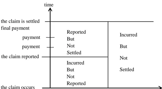
A claim is not always immediately reported to the insurance company when it occurs. Also, the final amount of a claim is not always known when the claim is reported. To better understand these situations, let us illustrate to some examples. In the accident insurance, this is often does not last a long time ago the claim is reported, but it can take a long time before the degree of disability is known, or death occurs as a result of accident. In the product liability insurance, it can take a long time before the damage is determinated and reported and assess to extent of the damage evaluated. Usually one has to await the outcome of litigation. In the fire insurance, the claim is generally reported early, but this claim can take long before it is settled. A claim that has occurred but is not yet reported, is called an IBNR claim. There are many reasons for predicting IBNR claims. One of these is rate-making. When attributing premiums on statistical experience, one should not ignore unsettled claims. The other reason is reserves. An unsettled claim consists of one or more future payments for which the insurance company has already assumed liability through the insurance contract, and therefore the company has to keep assets to cover these payments. Another reason is supervision. When appraising the financial strength of the insurance company, the unsettled claims should be taken into account.
Each of these aims impresses its own particular requirements on the prediction procedures, and as in addition the troubles are not similar for each portfolio, one would typically need various models and methods. By an IBNR reserve we mean a provision made to cover future payments on IBNR claims. These are illustrated in the following Figure 2.1.
Figure 2.1. The development of a claim.
Several estimators for IBNR reserve have been proposed in the literature, which are Chain Ladder, London Chain Ladder, Bornhuetter-Ferguson methods, Loss Ratio methods London Pivot and Cape-Cod. Under Solvency II it has become fashionable to consider reserving on stochastic claims reserving methods. After constituting the basic knowledge about the IBNR claim reserves, one of the most common methods for used to estimate IBNR claims is the chain ladder method will be given in the next section.
2.2 Chain Ladder
The main objective of chain ladder method is based on an algorithm which makes a point estimate of future claims. The chain-ladder method is simple and logical, and is widely used in casualty insurance. Despite its popularity, there are weaknesses inherent to this method. Most importantly, it does not provide information regarding the variability of the outcome. With the processing power of today’s computers, the simplicity of the method is no longer a valid argument. All the same, the chain-ladder method is frequently used by actuaries.
time Incurred But Not Reported Reported But Not Settled Incurred But Not Settled
the claim occurs the claim reported
payment payment the claim is settled final payment
* * * *
The majority of reserving methods are based on the run-off triangle. Information on claims is usually summarized in these triangles, either incremental triangles, or cumulated payments. It corresponds to an incomplete n × n matrix. Consider a triangle of data classified according to an index for accident year i, and an index for reporting delay j. We denote accident years by i {1, …, n} and development years by j {1, …, n}, where n N denotes the last observed accident year.
Accident year i
Development year j Calendar year i + j
Or ig in Y ea rs Development Years Reported Claims
Future Claims Developments
* * * *
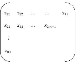
Information on claims is usually summarizes in payment triangles, either claim amounts, or cumulated payments. denotes the claim amounts where i denotes the accident year and j the development year. Then the set is:
{ }
The data may be presented as a run-off triangle:
Figure 2.2. Run-off triangles, where the triangle displays the claim amounts. The rows display the accident year (i) and the columns display the development year (j). The claims in the north-western triangle are known values; the chain-ladder algorithm seeks to estimate future claims in the south-eastern (empty) triangle.
… …
…
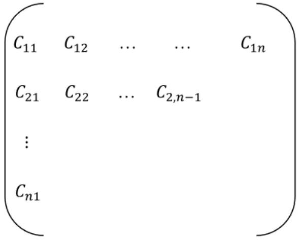
Let denote the cumulative claims. The accident year is the year the accident
occurs and the development year represents the reporting delay from when the claim occurred. The cumulative claim is
It may be presented as run-off triangle:
Figure 2.3. Run-off triangles, where the triangle displays the observed cumulative claims. The rows display the accident year (i) and the columns display the development year (j). The claims in the north-western triangle are known values; the chain-ladder algorithm seeks to estimate future claims in the south-eastern (empty) triangle.
… …
…
The problem is to find outstanding claims on the basis of past experience. In other words to predict future incremental claim amounts, fill in in the empty cells of the lower right hand triangle of claims. We call this region is target triangle. The chain ladder technique was conceived as a deterministic method for predicting claim amounts.
The method assumes that the cumulative claims for each year develop similarly by delay year, and estimates development factors as ratio of sums of cumulative claims with the same delay index. Consider here that and be the cumulative claims amount of accident year i, , after j years of development, . We assume
Thus the estimates of the development factor for the columns j is: ̂ ∑ ∑ for all
Hence, it becomes possible to estimate future payments using
̂ [ ̂ ̂ ]
This technique is based on fairly standard and completely dealing with positive claim amounts. If there are negative claims in the development triangle, this method cannot apply under these assumptions. At the next section concern about the use of the chain ladder method which is not limited by the existence of negative claims.
2.3 Mack’s Chain Ladder
Thomas Mack was the first to suggest a stochastic model for IBNR reserve estimation. His method is the most popular and practical method to solve this claim reserving problem. The principal reasons for that are: it is very basic and it gives exact results. The Mack's Chain-ladder (MCL) is a distribution-free method. It links consecutive cumulative claims with appropriate link ratios. Mack’s chain-ladder method calculates the standard error for the reserves estimates. The method works for a cumulative triangle , and cumulative claims of different accident period i are
independent. form a Markov chain. There exist development factors 0,
with 1 j n, such that for all 1 i n and all 1 j n hold:
( | ) ( | ) (2.6)
From the runoff triangle data C, the MCL predicts the growing factor from
column j to column j+1 by the use of the following estimator:
̂ ∑ ∑ =∑ ∑ (2.7)
Note that this estimator is in fact a weighted average of the observed individual development factors
⁄ .
The variance parameters , for all 1 j n-2 are estimated by the following unbiased estimator:
̂ ∑
̂ (2.8)
After computing the growing factors estimates, the IBNR total reserve can now be computed using the following unbiased estimator:
∑ ̂ ̂ (2.9)
2.4 Munich Chain Ladder
Munich chain ladder is an extension of Mack’s method that reduces the gap between IBNR projections based on paid (P) and incurred (I) losses. Mack has to be applicable to both triangles. Munich chain ladder adjusts the chain-ladder link-ratios depending if the momentary (P/I) ratio is above or below average. Munich chain ladder uses the correlation of residuals between P vs. (I/P) and I vs. (P/I) chain-ladder link-ratio to estimate the correction factor. The Munich chain ladder method will
therefore yield more reliable results for practically all portfolios where chain ladder calculation is appropriate for both the paid and incurred triangles.
2.5Bornhuetter-Ferguson Method
Bornhuetter-Ferguson method was first described by Bornhuetter and Ferguson (1972). The Bornhuetter-Ferguson method suggests predictors of the outstanding losses. By Klaus D. Schmidt and Mathias Zocher (2008) say:
“Every predictor is found by multiplying an estimator of the expected cumulative loss by an estimator of the percentage of the outstanding loss with respect to the ultimate one. The point that these methods aim at different target quantities can be neglected since predictors of ultimate losses can be converted into predictors of outstanding losses, and vice versa. However, a crucial difference lies in the fact that the chain ladder method proceeds from current losses while the Bornhuetter-Ferguson method is based on the expected ultimate losses, and this difference is connected with the sources of information which are taken into account: The chain-ladder method relies completely on the data contained in the run-off triangle. The Bornhuetter-Ferguson method restricts the use of the run-off triangle to the estimation of the percentage of the outstanding loss and uses the product of the earned premium and an expected loss ratio to estimate the expected ultimate loss. The striking point with the Bornhuetter-Ferguson method is the multiplicative structure of the predictors of the outstanding losses.”
3. MODELS
3.1 A Stochastic Model Underlying The Chain Ladder Technique
Renshaw and Verrall (1998) have criticized, there is association between the chain ladder technique and the stochastic model for incremental claims :
(3.1)
where:
(3.2)
and an assumption is that used in this paper. We assume throughout that:
∑ (3.3)
Note that for this assumption it is not assume that all the incremental claims are non-negative, but just that the column totals are non-negative. Also, the incremental claims are random variables. There are a number of points which should be made about this model. Kremer (1982) used the same structure but it is different from the distribution of model; Kremer used a lognormal distribution. Also, the specification of the Poisson modeling distribution does not mean that the model can only be applied to data which are positive integers. This means that the model can be applied to negative incremental claims, etc., and the results are always the same as those by the chain ladder technique (when ∑
Renshaw and Verrall (1998) obtained the maximum likelihood estimates for the model given by (3.1) and (3.2) using GLIM (Francis, Green & Payne, 1993). The
estimates of the total number of claims in each accident year may be obtained from the sums:
̂ ∑ ̂ ̂ ̂
where ̂ ̂ ̂ are the maximum likelihood estimates of the parameters.
is conditional likelihood which are estimates of { }. This
means that a claim with accident year index i, that is less than, or equal to, . Also, reported with delay index is j.
The estimates of { } are obtained using the following
conditional likelihood which is denoted by .This is the conditional probability that a claim with accident year index i and reported with delay index is j. For the accident year i given that is less than, or equal to, It is known from the usual supposition of stationarity, the probability that a claim is reported in each delay year does not depend on the accident year and is the (unconditional) probability that has been reported up to delay index year j. Then:
∑
where ∑ .
is the conditional likelihood which has conditions on the latest row totals . The multinomial distribution is used for obtaining to these data, and is given by:
∏ ∏ ∏
The fact that this likelihood gives the following estimates for the total number of claims:
̂ ∑ ̂
where ̂ is the estimate of obtained by maximizing
It can be shown that the equation (3.4) and (3.7), that is Poisson model estimates and conditional likelihood, give the same results.
It can be more convenient to use n-j+1 instead of equation in (3.7) accident year i which means it has been reported up to delay index j. Then the estimate is:
̂ ∑ ̂
This can be associated with the chain ladder estimates:
̂ ̂ ̂ ̂ where: ̂ ∑ ∑
Rosenberg (1990) derived a technique for obtaining the estimates { ̂ } which is recursive. Suppose that we have estimates of .
̂ ̂ ̂ ̂ ̂ ̂ Note that ̂
⁄ , which begins the recursion.
Verrall (1991) shown that a generalized linear model which obtains the same estimates of { } gives exactly the same results as the chain ladder technique, as the model (3.1) and (3.2), under assumption (3.3).
3.2 Claims Reserving When There Are Negative Values In The Runoff Triangle: Bayesian Analysis Using The Three-Parameter Log-Normal Distribution
A Bayesian model for the unobserved aggregate claim amounts and the necessary reserves for outstanding claims are presented in this section. The approach followed is set out in de Alba (2002a), where use in the presence of negative incremental claims is made of the three-parameter log-normal distribution to estimate outstanding claims reserves.As the mentioned by the previous sections, is random variable which represent the value of incremental claims amounts in the j-th development year of accident year i, i, j= 1, . . . , n. The random variable are known for i + j , and we let
( )
where is called the ‘‘threshold’’ parameter. If , then has a
( | ) { ( )√ { ( ( ) ) }
Crow and Schimidzu (1988) present the threshold parameter does not have restrictions except that ( ) must hold. The threshold parameter adjusts the negative incremental claim values so as to ensure ( ) , for i, j= 1, . . . , n, with i + j in this claims-reserving problem. Let us also assume that
( ) (3.14)
i, j= 1, . . . , n and i + j so that follows a three-parameter log-normal
distribution, denoted by with and
( | )
( )√ [ ( ( ) ) ]
( )
where is the usual indicator function.
Here and i, j= 1, …, n represent the accident year (row) and development year (column) effects, respectively. An unbalanced two-way analysis of variance (ANOVA) model corresponded by the model in equation (3.12). The certain restrictions must be imposed on the parameters to attain estimability in equation (2.4) that is well known in ANOVA. Verrall (1990) uses the assumption that .
All the observed values of , where ( ), and is the vector of parameters are contained if { } be a - dimension vector. The likelihood
function will be | if the product is over the known values, i, j= 1, . . . , n and i + j .
In de Alba (2002a) the maximum likelihood estimates first the threshold parameter , substitutes to define ( ̂), and then obtains the ‘‘profile’’
likelihood, ( | ̂) ( | ̂). Crow and Shimizu (1988, p.123) present the likelihood function with replaced by its ML estimator, say, ̂. Zellner (1971b) provides that the profile likelihood is used instead of the likelihood | | to carry out the Bayesian analysis, which then is done using results for a two-parameter lognormal distribution. Alba (2002a) presents the approach that the variability due to estimating is not taken into account in the inference process with the disadvantage. Because of this trouble the estimates of can be very unstable since it is well known that (see Cohen and Whitten 1980; Johnson, Kotz, and Balakrishnan 1994, chap. 14; Hill 1963). Alba (2006) used the full likelihood function | .
Alba (2006), to specify prior distributions, the parameters and must be specified to carry out the Bayesian analysis. Assume that a priori the parameters are independent, so that [∏ ] [∏ ( ) ]
The parameters are not modeled explicitly a priori and any dependence among the parameters will be reflected in the posterior distribution since it will be introduced by the sample data through the likelihood function. To obtained the posterior distribution as
As Alba (2006) mention in the below, hierarchical model, that exist at a first stage the data are specified to come from a given distribution, in
our case, will be used. To mention the second stage, the parameters are assumed to follow their own (prior) distributions, here ( ) and i, j=
2, . . . , n. Markov chain Monte Carlo (MCMC) simulation then will be used to
generate samples from the posterior distributions of the parameters as well as the predictive distribution of the reserves. Its implementation with the package Win
BUGS 1.4 (Spiegelhalter et al. 2001) or Open BUGS (http://
mathstat.helsinki.fi/openbugs/). The specification of the prior distributions followed is described in Alba (2006).
According to the characteristics of the parameter, a prior distribution can be specified using any distribution that is reasonable. It can use what are known as noninformative or reference priors which are distribution will be chosen to reflect our state of ignorance when there is no agreement on the prior information and there is a total lack of it. These are known as objective Bayesian inference under these circumstances. The values of the parameters in the prior distributions must be assumed to follow and in turn be specified (Zellner 1971a). This is easily done in WinBUGS (Scollnik 2001).
Alba (2006) mentioned to estimate (or obtain the distribution of) aggregate claims for the i-the accident year, i= 2, . . . , n, given in the development triangle. Recall that the cumulative claims are given by for ∑ for 1 Hence, it can be really interested in estimating i= 2, . . . , n given , i= 1, . . . , n t= 1, . .
. , n, with . Now let , for i= 2, . . . , n, where
is the accumulation of up to the latest development period and equals the total
aggregate outstanding claims corresponding to business year i, for i= 2, . . . , n. The required reserves corresponding to this business year can be obtained by quantile desired in the distribution of outstanding claims from the distribution of . Finally, from ∑ , that is the distribution of total aggregate outstanding claims, the required total reserves can be computed.
4. RESULTS
Claims reserves, a concept that is very important for financial stability of the insurance company. Some of the expiry of the insurance claims can be reported, even after many years, and the company reflected as a liability, damages, payment times in the socio-economic conditions of production of the policy conditions be very different from the calculation of provisions set aside for the claims of companies has led to the need to be very careful (Yaman 2005).
Actuarial literature, the predict for claims based on statistical analysis over deterministic method is being used which are Chain Ladder, London Chain Ladder, London Pivot, Cape-Cod and so on. The common feature of all these classical methods to group the available data within a triangular table. In this thesis, classical methods used for calculation of accurate observations and reserve estimation, regression analysis approach, based on the Chain Ladder method, the development triangle, even if some of the cells in the presence of negative values is to be applied and the best estimate of damage to the reserve.
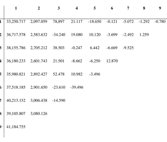
The data set used in the analysis is a set of claims data for Prof. R. L. Brown’s works from American Insurance Company. The insurance claims were organized by accident year and development year. It contained the number of reported claims, the number of claims that had not been reported, and the number of IBNR- claims. The first stage of the application data in Table 4.1 are collected in table triangle, as shown in Excel worksheet added.
Table 4.1. A set of claims data which is Prof. R. L. Brown’s works from American Insurance Company.
The following code in R programming language is transferred to R console from Excel worksheet:
negative <- read.csv("C:/Tez/negative.csv", header=F)
Then, the data have been converted to cumulative form for provide the necessary conditions in the section 3. These phases are typed in R console with the following code: 1 2 3 4 5 6 7 8 9 1 33,250.717 2,097.059 78,897 21.117 -18.650 -0.121 -5.072 -1.292 -0.780 2 36,717.578 2,583.632 -34.240 19.080 10.120 -3.699 -2.492 1.259 3 38,155.786 2,705.212 38.503 -0.247 6.442 -6.669 -9.525 4 36,180.233 2,601.743 21.501 -8.662 -6.250 12.870 5 35,980.821 2,892.427 52.478 10.982 -3.496 6 37,518.185 2,901.650 -23.610 -39.496 7 40,213.152 3,006.438 -14.590 8 39,105.807 3,080.126 9 41,184.755
n=dim(negative)[1] cumdata=negative for(i in 2:n){ for(a in 1:n){ cumdata[a,i]=cumdata[a,i]+cumdata[a,i-1] } }
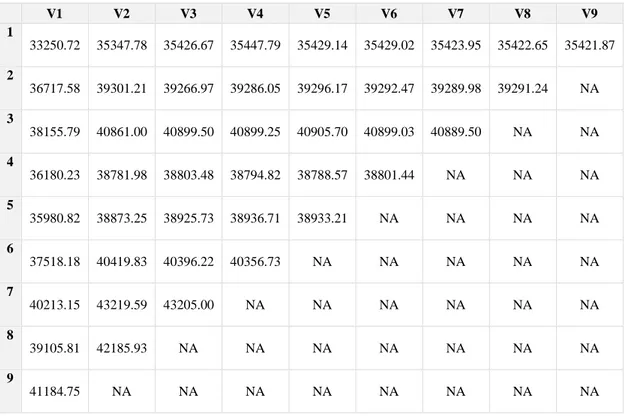
Table 4.2. A set of claims data which is converted to cumulative form in R.
V1 V2 V3 V4 V5 V6 V7 V8 V9 1 33250.72 35347.78 35426.67 35447.79 35429.14 35429.02 35423.95 35422.65 35421.87 2 36717.58 39301.21 39266.97 39286.05 39296.17 39292.47 39289.98 39291.24 NA 3 38155.79 40861.00 40899.50 40899.25 40905.70 40899.03 40889.50 NA NA 4 36180.23 38781.98 38803.48 38794.82 38788.57 38801.44 NA NA NA 5 35980.82 38873.25 38925.73 38936.71 38933.21 NA NA NA NA 6 37518.18 40419.83 40396.22 40356.73 NA NA NA NA NA 7 40213.15 43219.59 43205.00 NA NA NA NA NA NA 8 39105.81 42185.93 NA NA NA NA NA NA NA 9 41184.75 NA NA NA NA NA NA NA NA
The following code is obtained from the equations (3.11) and (3.12): p=1:n p[n]=negative[1,n]/cumdata[1,n] for (j in (n-1):1){ numerator=sum(negative[1:(n-j+1),j]) denominator=cumdata[1,n] for (k in 2:(n-j+1)){ denominator=denominator+(cumdata[k,(n-k+1)])/(1-sum(p [n:(n-k+2)])) } p[j]=numerator/denominator }
The following examples illustrate, { }:
j=10: j=9:
j=8: j=7:
Afterwards, the equation (3.7) is typed in R console, as shown below:
c_hat=1:n
c_hat[1]=cumdata[1,n] for (i in 2:n){
c_hat[i]=cumdata[i,(n-i+1)]/(1-sum(p[(n-i+2):n])) }
Table 4.3. The estimates for the total number of claims in R.
̂ ̂ ̂ ̂ ̂ ̂ ̂ ̂
Finally, the following code is typed to calculate the reserve: diagonal=NA for(r in 1:n){ diagonal[r]=cumdata[r,(n-r+1)] } reserves=c_hat-diagonal
As mentioned above, in the Bayesian approach, the known data in the upper triangle, x, are used to predict the observations in the target triangle by means of the posterior predictive distribution for outstanding claims in each cell:
( | ) ∫ ( | ) |
i= 1, . . . , n, j= 1, . . . , n, with
After the reserves for the outstanding aggregate claims are estimated as the mean of the predictive distribution, for each cell ( | ) must be obtained. Hence,
the Bayesian estimate of the total outstanding claims for year of business i is ∑ ( | ). The Bayesian ‘‘estimator’’ of the variance of outstanding claims (the predictive variance) for that same year is used to generate samples from the posterior distributions of the parameters as well as the predictive distribution of the reserves to derive analytically. This is where Markov chain Monte Carlo (MCMC) simulation proves to random observations for aggregate claims in each cell of the (unobserved) lower right triangle , i= 2, . . . , n, for j= 1, . . . ,
N. The resulting (predictive) values will include both parameter variability and
process variability. These predictive values can be used to compute the mean and variance of the reserves. To compute a random value of the total outstanding claims
can be obtained ∑
for j= 1, . . . , N. Also the mean and variance of total
outstanding claims can be accessed as
∑ ̅
5. CONCLUSION
As mentioned previously, for the claims data, Prof. R. L. Brown's study in American insurance company have been used. In previous years, taking into consideration the size of the incurred claims, for the periods which are not reported, stochastic model has been applied in R programming language.
In addition, the distributions of the data’s damages’ have been tested to conform with the distribution by using Minitab 14 package program and α <0.003 error level "to comply with the distribution of exponential distribution" showed us hypothesis cannot be rejected. Distributions of each term tested separately and according to the result, the most suitable distribution has been proved as exponential distribution. Due to the exponential distribution outcome claims reserves and standard errors have been calculated. Thereby, the differences between the sizes of claims that are informed which reported in prior periods and the size of claims that are calculated for the not reported periods have been determined.
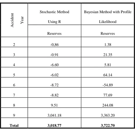
Table 5.1. Estimation of Reserves. Ac cid en t Ye ar Stochastic Method Using R
Bayesian Method with Profile Likelihood Reserves Reserves 2 -0,86 1.38 3 -0.91 21.35 4 -6.60 5.81 5 -6.02 64.14 6 -8.72 -54.89 7 -8.82 77.69 8 9.51 244.08 9 3,041.18 3,363.20 Total 3,018.77 3,722.70
The methods used for these reserves have been compared above in Table 5.1. As a result: the total reserve amount have been added from Alba's (2006) study "Bayesian Method with Profile Likelihood" is 3,722.70 and the total reserve amount which have been given and calculated in details on this study “Stochastic Method Using R” is 3,018.77. In this study the reserves in Bayesian Method with Profile Likelihood are not very close with the Stochastic Method Using R for this data.
A suggestion to be made based on this study is to provide insurance companies, whose payments are in big amounts, to establish their own risk models. Also, this study is to provide these companies to choose the best method according to the data they have obtained to calculate amounts of premium. Nevertheless, it is probable to face with the risks of paying big amounts premiums by standard methods the packaging program.
KAYNAKLAR DİZİNİ / BIBLIOGRAPHY
Alba, E., 2006, Claims reserving when there are negative values in the runoff
triangle: Bayesian analysis using the three-parameter log-normal distribution,
North American Journal, 10: 45-59.
Alba, E., 2002b, Bayesian estimation of outstanding claim reserves, North American Actuarial Journal 6(4): 1–20.
England, P.D., and Verrall R.J., 2002, Stochastic claims reserving in general
insurance,British Actuarial Journal8/3, 443-518.
England, P.D., and Verrall R.J., 2007, Predictive distributions of outstanding
liabilities in general insurance, Annals of Actuarial Science 1, 221-270.
England, P.D., 2002, Addendum to analytic and bootstrap estimates of prediction
errors in claims reserving, Insurance: Mathematics and Economics 31, 461-466.
Gamage J., Linfield J., Ostaszewski K., and Siegel S., 2007, Statistical Methods
For Health Actuaries IBNR Estimates, Society of Actuaries Health Section Research Project,1-85.
Gould I., 2008, Stochastic chain-ladder models in nonlife insurance, MSc Thesis,
University of Bergen, 114p (unpublished).
Hess, T., and Schmidt K., 2002, A comparison of models for the chain-ladder
method, Insurance: Mathematics and Economics, 31: 351-364.
Mack, T., 1991, A simple parametric model for rating automobile insurance or
estimating IBNR claims reserves, A Journal of the International
Mack, T., 1993, Distribution-free calculation of the standart error of chain-ladder
reserves estimates, A Journal of the International Actuarial Association Astin
Bulettin, 23/2, 213-225.
Mack, T., 1994, Which stochastic model is underlying the chain ladder method? Insurance: Mathematics and Economics, 15: 133-138.
Quarg, G. and Mack, T., 2008, Munich Chain Ladder: A Reserving Method that
Reduces the Gap between IBNR Projections Based on Paid Losses and IBNR Projections Based on Incurred Losses, Variance, 2:2, 266-299.
Renshaw, A., 1989, Chain ladder and inretactive modelling (claims reserving and
GLIM), J.I.A. 116, 559-587.
Renshaw, A., 1994a, Modelling the claims process in the precense of covariates, A Journal of the International Actuarial Association Astin Bulettin, 24,
265-285.
Renshaw, A., and Verrall, R., 1998, A stochastic model underlying the chain-ladder
technique, British Actuarial Journal, 4: 903-923.
Schmidt K., and Zocher M., 2008, The Bornhuetter-Ferguson principle, Casualty Actuarial Society, 2: 85-110.
Sundt, B., 1999, An introduction to non-life insurance mathematics,
Veröffentlichungen des Instittuts für Versicherungswissenschaft der Universität Mannheim, Karlsruhe, 172p.
Verrall, R., 1989, A state space representation of chain ladder linear model, J.I.A. 116, 589-610.
Verel, R., 1990, Bayer and emprirical Bayes estimation for the chain ladder model, A Journal of the International Actuarial Association Astin Bulettin, 20,
Verrall, R., 1991a, On the unbiased estimation of reserves from loglinear models, Insurance: Mathematics and Economics, 10, 75-80.
Verrall, R., 1991b, Chain ladder and maximum likelihood, J.I.A. 118, 489-499. Werner H., 2007, A Gamma IBNR Claims Reserving Model With Dependent
Development Periods , A Journal of the International