* Corresponding Author
Received: 13 March 2017 Accepted: 04 June 2017
The Relationship Between Adiabatic Electron Sound Speed and Electron Flux in the F-region of Ionospheric Plasma
Ali YEŞİL1,*, Kadri KURT2
1Fırat University, Faculty of Sciences, Department of Physics, 23119 Elazığ, Türkiye,
2MEB, Competition Authority Anatolian High School, Physics Teacher, 21120 Diyarbakır,
Türkiye, [email protected]
Abstract
In this study, the relationship between the electron flux and adiabatic electron sound speed were investigated with local time variations, using the real geometry of the earth’s magnetic field for both solstices (March 21 and September 23) and geographic latitudes in the ionospheric F-region. For these days, the electron flux was obtained as a
tensor. According to the results, yz=zy for both solstices. Furthermore, the magnitude
of the electron flux obtained at the autumn equinox is larger than the magnitude of the electron flux obtained at the spring equinox. In addition, a linear relation was found between the electron flux and the adiabatic electron sound speed.
Keywords: Electron Flux, Adiabatic Electron Sound Speed, Ionosphere.
İyonosferik Plazmanın F-Bölgesinde Adyabatik Elektron Ses Hızı ile Elektron Akısı Arasındaki İlişki
Özet
Bu çalışmada, İyonküre’nin F bölgesi için Dünya’nın manyetik alanının gerçek geometrisi kullanılarak kuzey yarımkürede adyabatik elektron ses hızı ile elektron akısı arasındaki ilişki coğrafik enleme bağlı olarak ekinoks (21 Mart ve 23 Eylül) günleri için yerel zamanla değişimleri incelenmiştir. Bu günler için elektron akısı matris olarak elde
Adıyaman University Journal of Science
dergipark.gov.tr/adyusci
ADYUSCI
38
edilmiştir. Elde edilen bulgulara göre, matris elemanlarından yz nin her iki gün
dönümünde de zy ye eşit olduğu görüldü. Ayrıca sonbahar ekinoksunda elde edilen
elektron akısının değeri, ilkbahar ekinoksunda elde edilen elektron akısı değerinden daha büyük olduğu görüldü. Bunun yanı sıra elektron akısı ile adyabatik elektron ses hızı arasında lineer bir ilişki belirlendi.
Anahtar Kelimeler: Elektron Akısı, Adyabatik Elektron Ses Hızı, İyonküre.
1. Introduction
Ionosphere is a natural plasma and an atmospheric layer starting from an altitude of 50 km and extending up to 1000km [4,7,8,12,15,16]. There are three significant processes affecting the change in particle density inside the ionosphere layer. The first one is charged particles coming from the Sun, ionizing the gases inside the atmosphere-increase in electron density, the second one is the chemical processes occurring at the ionosphere-decrease in electron density, and the third one is the transport processes arising from the gradients formed inside the ionosphere [12-16]. All three are complex processes in themselves. Ion densities show local variation for a variety of reasons. Due to their light mass, electrons, which are the most fundamental parameter of ionosphere during a collective motion, move faster than ions. Due to their heavier masses, ions remain behind the electrons. This separation leads to the formation of an electric field between the ions and electrons [1-3,5,9]. This electric field accelerates electrons and ions in opposite directions. After a certain time, due to the effects of the Coulomb force, the ions and electrons start to move together. This phenomenon is called ambipolar diffusion, which is not independent of acoustic effects [14].
When thermal effects (P) are added to the equation for the motion of the
particles of the ionosphere plasma, two phenomena occur. The first of these is the acoustic wave phenomenon, which consists of different types of sound waves and the second one is the kinetic phenomenon in which some particles move with the phase velocity or move close to the phase velocity [6,10,11,13]. Ions and electrons inside the fluid move at their own speed of sounds under the effect of the pressure gradient. In addition to this, due to long interactions of particles with the wave, they become resonant with waves. These interactions can lead to collisionless wave damping,
39
increase in amplitude of the wave or instabilities. When magnetic effects are included, new types of waves can emerge and instabilities may occur. Electron sound speed, which is an acoustic effect depends on density and temperature [14]. This speed is directly related with the conductivity of the medium, with the mobility of the particle and with diffusion. This relationship is expressed as:
i U / i 1 Ne T k i m T k D 2 e 2 0 e b e e b 0 and 2 0 μ Ne [4,7,11].
The Ionosphere shows significant variations according to local time (daily), seasons, altitude and location (lower latitude-equator, middle latitudes and higher latitudes-pole). Hence, while examining any ionosphere parameter, those parameters must be taken into account. In this work, the change of the electron flux matrix coefficients of the ionosphere’s F-region with respect to altitude (352.358 km average peak value for equinoxes), seasons (for both equinoxes) and latitude were investigated via local time.
2. Material and Method
In this section, adiabatic speed of sound of electron and electron flux matrix are derived. If we assume B≠0 in any medium, this medium is called anisotropic [7,8,12,14]. Since there is a nonzero magnetic field inside the ionosphere plasma, ionosphere plasma is anisotropic. At the northern hemisphere, if the real geometry of the Earth’s magnetic field is used, then the magnetic field becomes three-dimensional as shown in Figure 1 [1-3].
Figure 1. The geometry of Earth’s magnetic field (for northern hemisphere) [1,3]. d
40
Here, Bx BCosISind is By BCosICosd and Bz BSinI . I is the magnetic
depth and d is the magnetic declination angle. The other rotations that will be used throughout this study are the following:
c
: Electron cyclotron frequency. These frequencies are given as;
m eB ω x cx , m eB ω y cy and m eB ω z cz
depending on the plasma parameters. Flux density is found to be [4]:
α α α α α α n D -E) n ( μ t D D ν n U B (1)
via the equation of motion. Here
α α α α ν m q μ and α α b α ν m T k
D are mobility of the
charged particle and diffusion coefficient respectively [11]. Recasting the flux density as; U α n (2)
the electron flux tensor,
zz zy zx yz yy yx xz xy xx (3) is obtained.
The elements of the tensor for electron are given in the figure below.
2
x 2 2 e 1 xx A U 1 B , 2
z x y
e 1 xy A U B B B
y x z
2 e 1 xz A U B B B , 2
z x y
e 1 yx A U B B B
2
y 2 2 e 1 yy A U 1 B , 2
x z y
e 1 yz A U B B B 41
y x z
2 e 1 zx A U B B B , 2
x y z
e 1 zy A U B B B
2
z 2 2 e 1 zz A U 1 B ,
2 2
B 1 A 3. Results and Discussion
In this study, with the help of IRI program, the daily changes of the elements of
the electron flux matrix for different latitudes (lower latitudes 0-300 , middle latitudes
30-600 and higher latitudes 60-900), at 352 km for 23 September 1990 and at 358 km for
21 March 1990 where electron densities were maximum (hmF2) were investigated using the real geometry of the Earth’s magnetic field in the northern hemisphere (Figure 1).
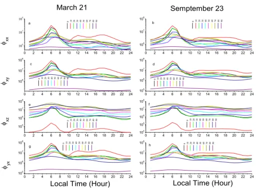
In Figure 2, the change of electron flux coefficients with latitude under accepted conditions for 21 March and 23 September is given. As it can be also seen from Eq. (3),
the magnitudes of the values yz and zy are equal for every time and latitude. The
change of xx with local time at the northern hemisphere for 21 March-23 September is
given in Figure 2 a and b. According to this, xx values take maximum values for
6:00-8:00 AM (sunrise) local time. Sudden decreases are being observed at 6:00-8:00-10:00 AM local time and small sudden increases and decreases after that time occurs for both equinoxes. Similar changes for the coefficients are being observed for each equinox
given in Figure 2. xx ,xy values for lower latitudes during both two seasons are greater
than that of middle and higher latitudes as displayed in Figure 2 a, b, c and d. The
values are maximum, particularly at the equator region (00 latitude). xz electron flux
reaches minimum values at lower latitudes whereas at higher latitudes it attains its maximum values, as it can be seen from Figure 2 d and f. At middle latitudes, electron
flux takes intermediate values. yx displays changes similar to xx with local time for
both two seasons, as demonstrated in Figure 2 g and h.
In previous studies, a direct relation between adiabatic electron sound speed and electron flux was not demonstrated, but there is a linear relation between adiabatic electron sound speed, diffusion and ionosphere conductivity [1-4]. Therefore, there is a strong similarity between the conductivity, the change of diffusion for an arbitrary
42
parameter at accepted conditions for all seasons and electron flux, depending on the adiabatic electron sound speed [5-14].
0 2 4 6 8 10 12 14 16 18 20 22 24 106 107 108 0 2 4 6 8 10 12 14 16 18 20 22 24 106 107 108 0 2 4 6 8 10 12 14 16 18 20 22 24 106 107 108 0 2 4 6 8 10 12 14 16 18 20 22 24 105 106 107 108 0 2 4 6 8 10 12 14 16 18 20 22 24 105 106 107 108 0 2 4 6 8 10 12 14 16 18 20 22 24 104 105 106 107 108 0 2 4 6 8 10 12 14 16 18 20 22 24 105 106 107 108 0 2 4 6 8 10 12 14 16 18 20 22 24 105 106 107 108 0 10 20 30 40 50 60 70 80 90 a b 0 10 20 30 40 50 60 70 80 90 0 10 20 30 40 50 60 70 80 90 c 0 10 20 30 40 50 60 70 80 90 d 0 10 20 30 40 50 60 70 80 90 e 0 10 20 30 40 50 60 70 80 90 f 0 10 20 30 40 50 60 70 80 90 g Semptember 23
Local Time (Hour)
yx
xz
xy
0 10 20 30 40 50 60 70 80 90
xx
Local Time (Hour) March 21
h
Figure 2. Local time variations in electron flux coefficients depending on the latitude.
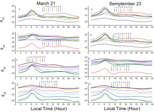
Figure 3 illustrates the daily change of electron flux coefficients with latitude. It
is observed that, all coefficients for all latitudes in the figure reach their maxima during sunrise and then reach a constant trend. The largest change for these maxima dips are observed at lower latitudes, whereas for higher latitudes the maxima are not drastically changed.
43 0 2 4 6 8 10 12 14 16 18 20 22 24 106 107 108 109 0 2 4 6 8 10 12 14 16 18 20 22 24 106 107 108 0 2 4 6 8 10 12 14 16 18 20 22 24 104 105 106 107 108 0 2 4 6 8 10 12 14 16 18 20 22 24 106 107 108 0 2 4 6 8 10 12 14 16 18 20 22 24 106 107 108 0 2 4 6 8 10 12 14 16 18 20 22 24 103 104 105 106 107 108 0 2 4 6 8 10 12 14 16 18 20 22 24 106 107 108 109 0 2 4 6 8 10 12 14 16 18 20 22 24 106 107 108 109 0 10 20 30 40 50 60 70 80 90 a b 0 10 20 30 40 50 60 70 80 90 0 10 20 30 40 50 60 70 80 90 c d 0 10 20 30 40 50 60 70 80 90 0 10 20 30 40 50 60 70 80 90 zz zx yz yy e 0 10 20 30 40 50 60 70 80 90 f 0 10 20 30 40 50 60 70 80 90 g 0 10 20 30 40 50 60 70 80 90
Local Time (Hour) Local Time (Hour)
Semptember 23 March 21
h
Figure 3. Change of electron flux coefficients with local time depending on the latitude.
Figure 3 a, b, c and d,
yy,
yz
zx and
zz show similar changes and for sametimes and latitudes they reach their maxima and minima Figure 3 e, f, g and h and Figure 2 e, f, g and h shows similar changes for all latitudes (lower, middle, higher) but display different magnitudes Figures 2 and 3 are consistent with the literature. So, the change in the coefficients of electron flux, diffusion, electron density and conductivity with local time are similar [1-16]. In parallel to that, the magnitudes of electron flux coefficients and diffusion coefficients have the same values [7,8,11-13,15].
4. Conclusions
This manuscript investigates on a daily and seasonal basis, whether there is a relation between the adiabatic electron sound speed and electron flux at heights of hmF2 by using the real geometry of the Earth’s magnetic field in the northern hemisphere. According to this;
yz=
zy for both seasons. Under the accepted conditions, this
44
this equality can mean the equality of diffusion, conductivity and mobility coefficients [11].
All electron flux values are at maximum at locations close to the
equator, during sunrise (6:00-8:00 AM local time) and between latitudes (0-200).
Here electron density displays an equatorial anomaly. The increase in flux at these latitudes and times can mean an increase in pressure gradient and in
acoustic effects [4]. Furthermore, the fact that at lower latitudes,
xx ,
xy,
,
yyand
yx electron fluxes take larger values compared with the other latitudes(middle and higher) and the fact that the transport processes here are more effective and there are more acoustic effects means that, this process gives rise to electron transport from the middle and higher latitudes to lower latitudes via temperature and density gradients. It is an important subject that is worth discussing.
xz ,
zx,
,
zz and
yz shows a contrasting result when comparedwith the second conclusion, which means, electron fluxes take larger values at higher latitudes and smaller values at lower latitudes. There could be two reasons why these components lead to this situation:
- Electron transport from higher latitudes to lower latitudes.
- Electron precipitation occurring at higher latitudes during solar activities [11-13].
All electron flux coefficients take larger values on 23 September
compared with the values they take on 21 March. It could be said that, acoustic effects are larger in the regions where conductivity and diffusion are higher.
The elements of the electron flux tensor directly depend on the
magnetic field. An increase in electron flux is analytically possible, when the magnetic field is large.
References
[1] Aydogdu, M., Ozcan, O., Effect of magnetic declination on refractive index
and wave polarization coefficients of electromagnetic wave in mid-latitude ionosphere,
45
[2] Aydoǧdu, M., Yeşıl, A., Güzel, E., The group refractive indices of HF waves
in the ionosphere and departure from the magnitude without collisions, Journal of
Atmospheric and Solar-Terrestrial Physics, 66(5), 343-348, 2004.
[3] Aydogdu, M., Ozcan, O., The possible effects of the magnetic declination on
the wave polarization coefficients at the cutoff point. Progress in Electromagnetic Research, PIER 30, 179-190. Abstract Journal of Electromagnetic Waves and
Applications, 14, 1289-1290, 2001.
[4] Bittencourt, J. A., Fundamentals of plasma physics. Springer Science & Business Media, 2013.
[5] Kutiev, I., Tsagouri, I., Perrone, L., Pancheva, D., Mukhtarov, P., Mikhailov, A., Andonov, B., Solar activity impact on the Earth’s upper atmosphere, Journal of Space Weather and Space Climate, 3, A06, 2013.
[6] Lastovicka, J., Akmaev, R. A., Beig, G., Bremer, J., Emmert, J. T., Global
change in the upper atmosphere. Science, 314(5803), 1253-1254, 2006.
[7] Rishbeth, H., Garriot, O. K., Introduction to Ionospheric Physics, Academic Press, New York, 175-186, 1969.
[8] Rishbeth, H., Physics and Chemistry of the Ionosphere, Contemporary Physics, 14(3), 229-249, 1973.
[9] Sagir, S., Atici, R., Ozcan, O., Yüksel, N., The effect of the stratospheric
QBO on the neutral density of the D region, Ann. Geophys., 58(3), A0331, 2015.
[10] Sagir, S., Karatay, S., Atici, R., Yesil, A., Ozcan, O., The relationship
between the Quasi Biennial Oscillation and Sunspot Number, Advances in Space
Research, 55(1), 106-112, 2015.
[11] Sagir, S., Yesil, A., Sanac, G., Unal, I., The characterization of diffusion
tensor for mid-latitude ionospheric plasma, Annals of Geophysics, 57(2), A0216, 2014.
[12] Schunk, R., Nagy, A., Ionospheres: physics, plasma physics and chemistry, Cambridge University Press, 2009.
46
[13] Yeşil, A., Sağır, S., Kurt, K., The Behavior of the Classical Diffusion
Tensor for Equatorial Ionospheric Plasma, BEU Journal of Science, 5(2), 123-127,
2016.
[14] Swanson, D. G., Plasma waves, Academic Press, San Dieogo, 1989.
[15] Yesil A., Sagir, S., Ozcan, O., Comparison of maximum electron density
predicted by IRI-2001 with that measured over Chilton station, E-Journal of New World
Sci. Acad, 4(3), 92-99, 2009.
[16] Kurt, K., Yeşil, A., Sağir, S., Atici, R., The Relationship of Stratospheric
QBO with the Difference of Measured and Calculated NmF2, Acta Geophysica, 64(27),
![Figure 1. The geometry of Earth’s magnetic field (for northern hemisphere) [1,3]. d](https://thumb-eu.123doks.com/thumbv2/9libnet/4487623.78806/3.892.349.611.829.1055/figure-geometry-earth-s-magnetic-field-northern-hemisphere.webp)